Online Full Text



Abstract- Present day state-of-art Automatic Speech Recognition (ASR) systems adapt to the environment through supervised learning techniques using labeled speech corpora.

ASR systems need huge-labeled data for adaptation and labeling such huge data is expensive and impracticable. On the other hand, Human Auditory Recognition (HAR) systems learn from “Everyday Speech” which represents the environmental conditions.

In this paper, we use unsupervised learning techniques to address the above adaptation problem. The new algorithm uses phonetic distance dissimilarity measures to enable ASR systems to learn from the test data. Hybrid HMM (Hidden Markov Model) and VQ (Vector Quantization) model is used to hold the knowledge base similar to its counterparts with the HAR system. Multi-Layer Code Book (MLCB) is used to optimize the search space.

The new algorithm is tested with data sets taken from CMUDICT and the test results have shown significant improvements in Word Error Rate (WER) measurements. The adaptation process using unsupervised learning algorithm is inexpensive, automated and faster compared to the existing techniques.

Index Terms—unsupervised learning, adaptation, ASR systems, Multi-layer code book

I. INTRODUCTION

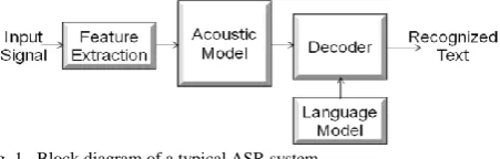
LOCK diagram of a typical ASR system is given in Figure 1. It consists of four modules – Feature Extraction module, Acoustic Model (AM), Decoder module and Language model (LM).

Fig. 1. Block diagram of a typical ASR system

The input waveform is converted into a set of feature parametric vectors. Mel-frequency Cepstral Coefficients

Manuscript received December 23, 2013; revised January 22, 2014. Akella Amarendra Babu is Research Scholar with JNIAS-JNTUA, Andhra Pradesh, India (phone: +91-9849934000; e-mail: aababu.akella@ gmail.com).

Yellasiri Ramadevi is Professor with the Computer Science and Engineering Department, Chaitanya Bharati Institute of Technology, Hyderabad, Andhra Pradesh, India (e-mail: [email protected]).

Akepogu Ananda Rao is Director and Professor with JNTUA, Anantapuramu, Andhra Predesh, India (e-mail: akepogu @ gmail.com).

(MFCC), its first order delta MFCC and second order delta MFCC are used for feature extraction [3], [5], [9]. The various techniques used to improve the parametric representation are given in the Table I.

TABLE I

FEATURES IMPROVEMENT TECHNIQUES Algorithm Purpose Recursive Least Squares (RLS)

Vector Taylor series (VTS) Noise cancellation

Short –time Energy (STE) Zero Crossing Rate (ZCR) Frame based Teager’s Energy (FTE) Energy Entropy Feature (EEF)

End point detection, and Speech segmentation

Mel Frequency Cepstral Coefficient (MFCC)

Perceptual Linear Prediction (PLP) Coefficients

Cepstral mean subtraction (CMS)

Feature extraction

RASTA filtering For Noisy speech

Principle Component Analysis (LCA) Linear Discriminant Analysis (LDA)

Feature Trans-formation

Acoustic Model (AM) converts the speech parametric vectors into corresponding phoneme sequences. Hidden Markov Models (HMM) are used for acoustic modeling [10], [16]. Various learning and decoding techniques are given in the Table II.

TABLE II

LEARNING AND DECODING TECHNIQUES

Maximum Likelihood estimation (MLE)

Maximum a Posteriori (MAP)

Supervised Learning methods

Maximum Mutual Information Estimation (MMIE)

Mini Classification Error (MCE)

discriminative training

Back Propagation Training MLPs

Vector Quantisation (VQ) K-Means Algorithm Expectation Max (EM) Algorithm

Unsupervised Training

Classification and Regression

Trees (CART) Pattern recognition

Dynamic Programming DTW

Forward Algorithm, Viterbi Algorithm, Baum – Welch Algorithm

HMM Evaluation, Decoder

Unsupervised Adaptation of ASR Systems

Using Hybrid HMM / VQ Model

Akella Amarendra Babu,

Member, IAENG,

Yellasiri Ramadevi,

Member, IAENG

, and

Akepogu Ananda Rao,

Member, IAENG

Decoder converts the phoneme sequences into words and uses Language Model (LM) for semantic validation [19], [21].

Adaptation of ASR systems is the inbuilt capability to discern and learn while it is being tested [1], [8], [17], [18]. It will make use of the everyday speech which available while the ASR system is under use for learning new words and new pronunciations. Since the process is online, it does not have the overheads of delay and expenses for labeling the speech corpora [6], [7].

In this paper, we presented an algorithm which uses data driven unsupervised methods to learn from the test data. The size of search space for finding the word hypothesis corresponding to the input phoneme sequences is optimized using multi-layer code book architecture. This paper is organized into six parts. Part II gives a brief overview of the related work. Part III describes the architectural design of the proposed adaptive ASR system. Design of Multi-layered Code Book is described in part IV. Part V covers the adaptation algorithm and part VI deals with the implementation details and results.

II. REVIEW OF RELATED WORK

In a closed vocabulary ASR systems, Out of Vocabulary (OOV) words and words with different pronunciations, encountered during recognition, will result in errors. A semi-supervised learning method was suggested by Raj Reddy et al [11]. In a dictation machine, the user corrects the erroneous word, and if the corrected word is OOV, that word is added to the vocabulary so that during future references, the word is correctly recognized. A set of n-best variants of pronunciations is derived for each word from its orthographic spelling. Each word in the n-best list and the acoustic waveform corresponding to that are aligned and probability based on maximum likelihood is calculated. Further, the phonetic transition penalty is calculated from the phone transition costs. Above three scores are multiplied to derive the combined score corresponding to each hypothesis and the highest ranking pronunciation is selected as the base-form pronunciation for that word.

T. Holter et al [12] developed an algorithm which creates pronunciations for various words using maximum likelihood criteria. The spoken words are converted to phoneme sequence and compared with the pronunciations in the pronunciation dictionary. The Maximum likelihood approach is adapted to create a single base-form for each word. Some words show variations of pronunciations among speakers. In such cases, more than one pronunciation is used to represent the words. Some words inherently show large variability in pronunciation, in which case, multiple pronunciations are used to represent those words.

Alex S. Park and James R. Glass described an off-line unsupervised learning method. It assumes that there is enough regularity in the acoustic speech which makes it possible to identify all lexical units from raw data [13]. Waveform segments with similar patterns are identified and grouped together and decoded. The process of generating lexical units is carried out off-line. The recorded classroom lecture of one hour duration is taken as test data.

Amos Tversky described various methods of measuring distances between objects based on the comparison of the features [2], [4]. The objects are represented as a set of features. The feature sets of two objects are compared. The super set of features contains all the features representing both the objects. It contains three sub-sets. One sub-set comprises of the features which are common for both the objects and the other two sub-sets comprise of the features which are exclusive to the respective objects. The ratio between the number of common features and the total number of features gives the similarity between the two objects.

John Nerbonne et al compare various European dialect words by measuring the phonetic distances [20]. The phonetic distance between a pair of phonemes can be estimated by calculating the difference between the features. Manhattan distance is the sum of differences between the feature vectors. The Euclidean distance between two phonemes is calculated as the square root of the sum of squared distances. The third method is the Pearson correlation coefficient method. The distance is measured as 1 – r where r is the correlation coefficient.

Stefan Schaden [22] suggested weighted overlapping of the features as the measure of the cost of substitution and uses weighted Jaccard coefficient to calculate the substitution cost. It is the ratio between the number of the features which are not common to both phoneme features and the total number of features. The ratio is multiplied by a weight which is calibrated for optimum results.

The Levenshtein distance is the distortion between two phoneme sequences. The two phoneme sequences are aligned and the alignment which gives with minimum distance is selected. The edit distance is measured in terms three operations. They are insertion cost, deletion cost and substitution operations. The cost of substitution operation is the distance between the phoneme pair. The cost of substitution operation will be different for different phoneme pairs. The substitution cost for all pairs of phonemes is added and the average substitution cost is calculated. The cost of insertion or deletion operation is calculated as half of the average substitution cost [23].

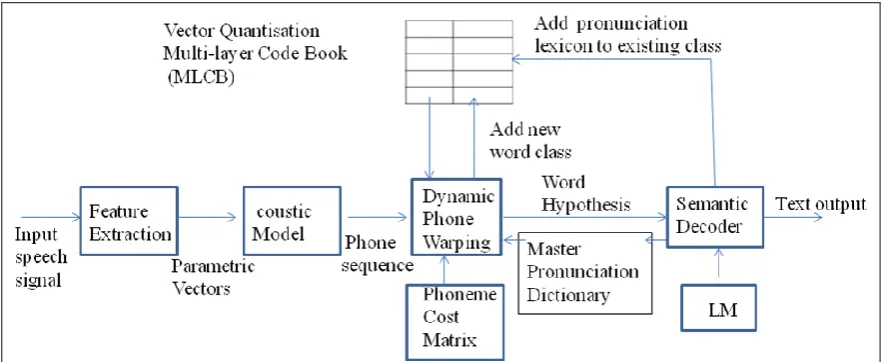
III. ADAPTATION ASR SYSTEM

Fig. 2. Block diagram of Adaptation ASR System

A. MLCB Module

This module implements a multi-layered Code Book. It is the space for storing the vocabulary W along with the corresponding pronunciation lexicon.

Pw ={Bm,(n)} m =1, …, M; n =1, …, N (1) Where Pw is the pronunciation lexicon, for the vocabulary of size W. Bm,(n) is the nth base-form of word m.

The architecture of MLCB is given in Figure 7 and is discussed in Part IV.

B. Phoneme Cost Matrix

Phoneme distance cost matrix is computed using articulatory features corresponding to various phonemes. The substitution cost between a pair of phonemes is calculated using the differences between the articulatory features of the two phonemes as a fraction of the total number of the articulatory features. The cost matrix is shown in Figure 3. The cost of deletion (Insertion) is calculated as half of the average substitution costs.

Fig. 3. Phoneme cost matrix for Standard English phoneme set

C. Dynamic Phone Warping (DPW) Module

It is the core of the Adaptation Subsystem. The DPW module calculates the phonetic distance between the analysis phoneme sequence Wa and the pronunciation baseforms Bm,(n) [14]. The n-best list of words is selected based on minimum distance criteria. The hypothesis word is given by

Dmin =Argmin (d (Wa, Bm,(n))) for all words in W (2) Wh = Word m corresponding to Dmin (3) The distance between two phoneme sequences, Sequence A and Sequence B is calculated by using dynamic programming technique. The length of Sequence A is M

and the length of Sequence B is N. The Sequence A has M phonemes, {P1, P2, …, Pm} and the Sequence B has N phonemes {P1, P2, …, Pn}. The first step is the alignment of the two sequences for the lowest score. The procedure is as under:

 Allot a two dimensional matrix, D with M rows and N columns. Allot one row for each phoneme in Sequence A and one column for each phoneme in Sequence B.

 D(i,j) is (i,j)th entry in the matrix D.

 D(i,j) is assigned a value as the calculations progress.  D(i,j) is the optimal score for i phonemes in sequence A and for j phonemes in sequence B.

 The first row and the first column of the D matrix are initialized as under:

--- for i=1 to length(Sequence A)

D(I,1) <- C*I Where C is cost of insertion (Deletion) for j= 1 to length(Sequence B)

D(1,j) <- C*j

---

 The remaining entries of the D matrix are calculated using following equation:

D(i,j) = min ((Di-1, j-1) + C(Ai, Bj), Di-1,j + C, Di, j-1+C) (4) Where C(Ai, Bj) is the cost of substituting Phoneme Bj for phoneme Ai. These values are taken from the phoneme cost matrix.

After all the values in the D matrix are computed, the value in the bottom right hand corner gives the minimum score for any alignment of phones between sequence A and Sequence B.

The actual alignment between Sequence A and Sequence B can be determined by back-tracking from the bottom right hand corner as under:

 In case, the choice of the equation (4) is the value corresponding to (Di-1, j-1) + C(Ai, Bj), then phoneme Ai and Bj are aligned.

 In case, the choice is the value corresponding to (Di-1,j + C), then Ai is aligned with a gap. It means that there is a cost of insertion.

there is a cost of deletion.

The DPW algorithm is run on the vocabulary taken from CMUDICT. The extract of three test cases is given in the Table III.

TABLE III

PHONETIC DISTANCES BETWEEN DIFFERENT WORDS AND THE SAME WORDS WITH DIFFERENT PRONUNCIATIONS

S. No. Word Pronunciation Distance

1 ACTIVISTS AE K T AH V AH S T S 0.00

2 ACTIVISTS(1) AE K T IH V IH S T S 0.08

3 ANNUITY AH N UW IH T IY 0.26

Test case 1

Sequence A: AE K T AH V AH S T S

Sequence B: AE K T AH V AH S T S

D Matrix = AE K T AH V AH S T S

0.00 0.18 0.36 0.54 0.72 0.90 1.08 1.26 1.44 1.62 AE 0.18 0.00 0.54 0.72 0.90 1.08 1.26 1.44 1.62 1.80 K 0.36 0.54 0.00 0.90 1.08 1.26 1.44 1.62 1.80 1.98 T 0.54 0.72 0.90 0.00 1.00 1.44 1.62 1.80 1.62 2.16 AH 0.72 0.90 1.08 1.00 0.00 1.00 1.44 1.98 2.16 1.98 V 0.90 1.08 1.26 1.44 1.00 0.00 1.00 1.80 2.34 2.52 AH 1.08 1.26 1.44 1.62 1.44 1.00 0.00 1.00 2.00 2.70 S 1.26 1.44 1.62 1.80 1.98 1.80 1.00 0.00 1.00 2.00 T 1.44 1.62 1.80 1.62 2.16 2.34 2.00 1.00 0.00 1.00 S 1.62 1.80 1.98 2.16 1.98 2.52 2.70 2.00 1.00 0.00 Phonetic Distance = 0.00

Fig. 4. Phonetic distance between two sequences with the same pronunciation. The distance is zero.

Test case 2

Sequence A: AE K T AH V AH S T S

Sequence B: AE K T HI V HI S T S

AE K T AH V AH S T S

0.00 0.18 0.36 0.54 0.72 0.90 1.08 1.26 1.44 1.62 AE 0.18 0.00 0.54 0.72 0.90 1.08 1.26 1.44 1.62 1.80 K 0.36 0.54 0.00 0.90 1.08 1.26 1.44 1.62 1.80 1.98 T 0.54 0.72 0.90 0.00 1.00 1.44 1.62 1.80 1.62 2.16 IH 0.72 0.90 1.08 1.00 0.36 1.36 1.80 1.98 2.16 1.98 V 0.90 1.08 1.26 1.44 1.36 0.36 1.36 2.16 2.34 2.52 IH 1.08 1.26 1.44 1.62 1.80 1.36 0.72 1.72 2.52 2.70 S 1.26 1.44 1.62 1.80 1.98 2.16 1.72 0.72 1.72 2.52 T 1.44 1.62 1.80 1.62 2.16 2.34 2.52 1.72 0.72 1.72 S 1.62 1.80 1.98 2.16 1.98 2.52 2.70 2.52 1.72 0.72 Phonetic Distance = 0.08

Fig. 5. Phonetic distance between two different pronunciations of the same word “ACTIVISTS”. The distance is less than Dcut-off.

The test case results show that the DPW algorithm initializes and fills up all the values of the D matrix. The value at the bottom right hand corner is normalized with the number of phonemes on the longest sequence. The normalized value gives the phonetic distance between the two phoneme sequences.

Test case 1 shows the DPW results between the phoneme sequences of the same word, “ACTIVISTS”. The phoneme sequences match with each other. Therefore, the phonetic distance between the two sequences is zero.

Test case 2 gives the DPW results between the phoneme sequences of the same word, but with different pronunciations. The phonetic distance is 0.08, which is less than the Dcut-off value. Therefore, the phoneme sequence under test is taken as a variation of pronunciation of the hypothesis word.

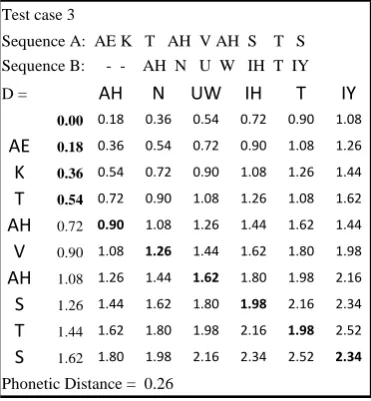
Test case 3 shows the results of the DPW results of two phoneme sequences corresponding to two different words. The phonetic distance is more than the Dcut-off value. Therefore, the phoneme sequence under test is taken as corresponding to an OOV word and pronunciation dictionary is searched for a new word.

Test case 3

Sequence A: AE K T AH V AH S T S

Sequence B: - - AH N U W IH T IY

D = AH N UW IH T IY

0.00 0.18 0.36 0.54 0.72 0.90 1.08

AE 0.18 0.36 0.54 0.72 0.90 1.08 1.26

K 0.36 0.54 0.72 0.90 1.08 1.26 1.44

T 0.54 0.72 0.90 1.08 1.26 1.08 1.62

AH 0.72 0.90 1.08 1.26 1.44 1.62 1.44

V 0.90 1.08 1.26 1.44 1.62 1.80 1.98

AH 1.08 1.26 1.44 1.62 1.80 1.98 2.16

S 1.26 1.44 1.62 1.80 1.98 2.16 2.34

T 1.44 1.62 1.80 1.98 2.16 1.98 2.52

S 1.62 1.80 1.98 2.16 2.34 2.52 2.34

Phonetic Distance = 0.26

Fig. 6. Phonetic distance between two different words “ACTIVITS” and “ANNUITY”. The distance is more than Dcut-off

D. Semantic Decode module

This module decodes the final word Wf output from the n-best hypothesis words, based on the following rules

Wf = Wh if 0 < Dmin ≤ Dcut-off (5) = Woov if Dmin > Dcut-off (6)

Dcut-off is the cut off value of the phonetic distance. If Dmin is more than D cut-off value, it is categorized as OOV.

In case Dmin value is less than or equal to Dcut-off value, the hypothesis word is considered as the pronunciation lexicon variant of the hypothesis word and the pronunciation lexicon corresponding to Analysis word Wa is added to MLCB corresponding to the hypothesis word.

In case, Dmin value is more than Dcut-off value, then the analysis word is considered as OOV of MLCB and Wh is discarded. The master pronunciation dictionary is searched for semantically suitable word Woov. The Woov is then enrolled into the MLCB for future references.

In case, Dmin value is equal to zero, the pronunciation phoneme sequence of the analysis word, Wa is perfectly matching with one of the pronunciation lexicon of the hypothesis word, Wh, and so the Wh is considered as correct and is output as Wf.

word is discarded. The pronunciation dictionary is searched to get a new word and the new word is enrolled into the MLCB. It results in an increase in WER and the consequent process overhead. On the other hand, in case the Dcut-off value is more than the optimum value, then analysis phoneme sequence corresponding to OOV words are categorized as pronunciation variations of hypothesis words and the semantic rules of the language model are applied to decide the context. It results in increase WER and the process overhead. Therefore, the value of Dcut-off is critical to the optimum performance of the Adaptation ASR system. The value of Dcut-off is decided empirically.

E. Language Model (LM)

The bi-gram grammar rules are used for the preparation of language model. The Semantic decoder uses the language model rules while deciding the semantic context.

F. Master Pronunciation Dictionary

CMU’s Pronouncing Dictionary version 0.07a is used as a master pronunciation lexicon database [15]. It contains approximately 133,300 plain text words which are mapped to their pronunciation phonetic strings. It has approximately 8500 words which provide two or more alternate pronunciations. In case an OOV word is encountered, the semantic decoder searches the master pronunciation dictionary for a semantically correct word which meets the criteria of minimum phonetic distance. The new word is enrolled into MLCB for future references.

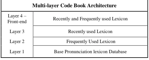
IV. DESIGN OF MULTI-LAYER CODE BOOK (MLCB) When the analysis phoneme sequence does not exactly match with the pronunciation lexicon in MLCB, there are two possibilities. First possibility is that the phoneme sequence is a pronunciation variant of a word class in MLCB. The other possibility is that it is an OOV word. In both the cases, a new lexicon or a new word class is enrolled into the MLCB and the size and search space of the codebook increases as the enrolment progresses. Multi-Layered Code Book (MLCB) architecture is used to keep the current search space optimal to achieve high recognition performance. MLCB architecture is given in the Figure 7.

Fig. 7. MLCB Architecture

V. ALGORITHM A. Step 1: Initialization

 Initialize Layer 4 with 10 words for bootstrapping.  Prepare test data with different pronunciation lexicon  Build Language model

B. Step 2: Iteration

 Generate phone sequences corresponding to analysis words from test data.

 Compute phonetic distance between the analysis word and all lexicons in the MLCB layer 4.

 In case the Dmin is non-zero, search layer 3, 2 and 1.  Generate word hypothesis.

C. Step 3: Decision

 In case, Dmin is zero, consider hypothesis word as Final word and output the text.

 In case, Dmin is greater than zero and less than Dcut-off, check for the context using semantic rules.

 If the word hypothesis matches the context, then enroll the corresponding pronunciation lexicon into the MLCB.  In case, the Dmin value is more than Dcut-off value or the Hypothesis word is not matching the semantic rules, then search for a new word in the master pronunciation dictionary which matches the semantics with less than Dcut-off value and enroll the word and the corresponding lexicon as a new class into MLCB.

D. Step 4

 Iterate step 2 and 3 for all the input data.

VI. IMPLEMENTATION

Adaptation ASR sub-system simulated using Java. CMU Sphinx tools are used to obtain the phoneme sequence for the word in the test data. The distances between these phoneme sequences and all the pronunciation sequences in the MLCB are measured using DPW. The distance is measured on the scale from zero to one. The distance between two exactly matching phoneme sequences is zero and the maximum distance between two different phoneme sequences is one.

Analysis of the experimental results show that the distances between the base-form pronunciation and the other variant pronunciations lie between zero and 0.9. Therefore, the cut-off distance (Dcut-off) is empirically fixed at 0.9.

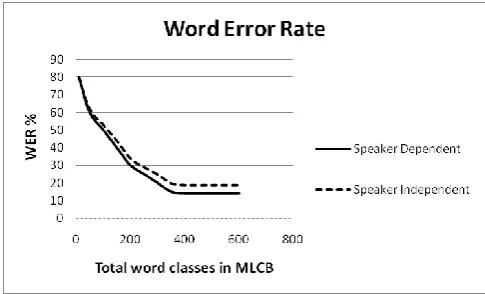
The life cycle of the adaptation process has two phases – learning phase and stable phase. In the learning phase, the ASR system is in the process of adding new pronunciations and new words from the input test data. The WER is high in the beginning of the learning phase and reduces as the input test data increases.

The stable phase starts when all the frequently used words are enrolled. The WER decreases to the lowest level. Each speaker has a fixed set of vocabulary. Therefore, when the input data is speaker dependent, the new word enrolments are at minimum level and the WER becomes flat. However, when the input data is speaker independent, there will be new word enrolments and new pronunciations. Therefore, the WER is more when compared to speaker dependent input data. The experimental results are shown in Figure 8. CMU pronunciation dictionary version 0.07a is used to create data corpus. The test data set is prepared using 200 commonly used words.

Multi-layer Code Book Architecture

Layer 4 –

Front-end Recently and Frequently used Lexicon

Layer 3 Recently used Lexicon

Layer 2 Frequently Used Lexicon

Fig. 8. WER vs Number of words enrolled in MLCB

VII. CONCLUSIONS

In everyday life, we face people with the different accent, adverse environmental conditions which add noise, distortion, Lombard and also we hear new words which are not heard earlier. While human beings adapt to the “Everyday Speech” based on the semantic context of the words in a sentence and remember the same, Automatic Speech Recognition (ASR) systems lack this capability. ASR systems need huge-labeled data for adapting to the environment which is impracticable. Performance of ASR systems degrades considerably when there is a slight variation in environmental conditions under which it is trained.

The proposed algorithm uses unsupervised learning techniques for adapting the easily available “Everyday Speech” like its counterparts with Human auditory Recognition (HAR) capabilities. Word-to-word phonetic distance is used to recognize words with the different accent and the word semantic context is used to validate the words and add new words into the vocabulary.

“Everyday Speech” is available in abundance online and ASR systems with unsupervised learning capabilities can adapt themselves for different prosodic accents and environmental conditions. The adaptation process using unsupervised learning algorithm is inexpensive, automated and faster compared to the existing techniques.

ACKNOWLEDGMENT

We thank all the research scholars of ROSE laboratory for their valuable suggestions and contributions.

REFERENCES

[1] Janet M. Baker, Li Deng, Sanjeev Khudanpur, Chin-Hui Lee, James Glass, and Nelson Morgan, “Historical Developments and future directions speech recognition and understanding”, IEEE Signal Processing Magazine, Vol 26, no. 4 78-85, Jul 2009.

[2] Oliver Pietquin and Thierry Dutoit, “A probabilistic framework for dialog simulation and optimal strategy learning”, IEEE Transactions on Audio, Speech and Language Processing, Vol 14, No 2, Mar 2006. [3] Khaled Abdalgadar and Andrew Skabar, “Unsupervised

similarity-based word sense disambiguation using context vectors and sentential word importance”, ACM Transactions on Speech and Language Processing, Vol 9, No 1, Article 2, May 2012.

[4] Amos Tversky, “Features of Similarity” Psychological Review, Vol 84, Number 4, July 1977.

[5] L. Rabiner, B. Juang and B Yegnanarayana, Fundamentals of Speech Recognition, Prentice Hall, Englewood Cliffs, N.J., 2010.

[6] N.A. Chomsky, “Knowledge of Language: Is Nature, Origin, and Use. Praeger”, New York, NY, 1986.

[7] P.W. Jusczyk, “The Discovery of Spoken Language. MIT Press/Bradford Books”, Cambridge MA, 1997.

[8] F. Pereira and Y. Schabes, “Inside-outside Re-estimation from Partially Bracketed Corpora.” 30th Annual Meeting of the Association for Computational Linguistics, pages 128–135, Newark, Delaware, 1992. Association for Computational Linguistics. [9] Nelson Morgan, “Deep and Wide: Multiple Layers in Automatic

Speech Recognition”, IEEE Transactions on Audio, Speech and Language Processing, Vol. 20, No. 1, January 2012

[10] Issam Bazzi and James Glass, “A MULTI-CLASS APPROACH FOR MODELLING OUT-OF-VOCABULARYWORDS”, Proceedings of the 7th International Conference on Spoken Language Processing, Sep. 16-20, 2002, Denver, Colorado, pp. 1613-1616.

[11] Gopala Krishna Anumanchipalli, Mosur Ravishankar and Raj Reddy, ”Improving Pronunciation Inference using N-Best list, Acoustics and Orthography ”, in Proceedings of IEEE Intl. Conf. on Acoustics, Speech and Signal Processing (ICASSP), Honolulu, USA, 2007. [12] T. Holter and T. Svendsen, “Maximum likelihood modelling of

pronunciation variation,” Speech Commun., vol. 29, no. 2-4, pp. 177–191, 1999.

[13] Alex S. Park, Member, IEEE, and James R. Glass, Senior Member, IEEE, “Unsupervised Pattern Discovery in Speech”, IEEE Transactions On Audio, Speech, And Language Processing, Vol. 16, No. 1, January 2008.

[14] Sungjin Lee and Maxine Eskenazi, “An Unsupervised Approach to User Simulation: Toward Self-Improving Dialog Systems”, Proceedings of the 13th Annual Meeting of the Special Interest Group on Discourse and Dialogue (SIGDIAL), pages 50–59, Seoul, South Korea, 5-6 July 2012.

[15] Ben Hixon, Eric Schneider, Susan L. Epstein, “ Phonemic Similarity Metrics to Compare Pronunciation Methods”, INTERSPEECH 2011, 28-31 August 2011, Florence, Italy.

[16] Xinguang Li, Jiahua Chen, Zhenjiang Li, “English Sentence Recognition Based on HMM and Clustering”, American Journal of Computational Mathematics, 2013, 3, 37-42.

[17] Anand Venkataraman, “A Statistical Model for Word Discovery in Transcribed Speech”, 2001 Association for Computational Linguistics, Volume 27, Number 3, pp 351 -372.

[18] Roger Argiles Solsona, Eric Fosler-Lussier, Hong-Kwang J. Kuo, Alexandros Potamianos, Imed Zitouni, “Adaptive Language Models For Spoken Dialogue Systems”, 2002 IEEE, pp 37-40.

[19] Huang, Acero, Hon, “Spoken Language Processing Guide to Algorithms and System Development”, PH, 2001.

[20] John Nerbonne and Wilbert Heeringa, “Measuring Dialect Distance Phonetically”, Alfa-informatica, BCN, 1997.

[21] Tao Tao, Su-Youn Yoon, Andrew Fister, Richard Sproat and ChengXiang Zhai, “Unsupervised Named Entity Transliteration Using Temporal and Phonetic Correlation”, Proceedings of the 2006 Conference on Empirical Methods in Natural Language Processing (EMNLP 2006), pages 250–257, Sydney, July 2006.

[22] Stefan Schaden, “Evaluation of Automatically Generated Transcriptions of Non-native Pronunciations using a Phonetic Distance Measure,” in Proceedings of LREC 2006, Genova, Italy, 006.