Hybrid Water Cycle Algorithm for Attribute Reduction Problems

D

Abstract—Attribute reduction in rough set theory is an important feature selection method. Since attribute reduction is an NP-hard problem, it is necessary to investigate fast and effective approximate algorithms. This paper presents a improve of water cycle algorithm (IWCA) for rough set attribute reduction, by hybrid water cycle algorithm with hill climbing algorithm in order to improve the exploitation process of the WCA. The idea of the WCA as an optimization algorithm was derived from nature, after examining the whole water cycle process which involves the flow of rivers and streams to the sea in the natural world. The IWCA has been tried on the public domain datasets that are obtainable in UCI. From the results of the experiments, it has been shown that the suggested method performs equally well or even better than other methods of attribute selection.

Keywords: Attribute Reduction. Improve Water Cycle Algorithm, Rough Set Theory, Hill Climbing Algorithm

I. INTRODUCTION

ue to the rapid increase in electronic information, the problems encountered in attempts to extract knowledge from the large space data have received much attention in the sphere of data mining. The Rough Set Theory (RST) is regarded as the main source of attribute reduction and the most efficient tool for extracting useful knowledge and data [1]. The role of attribute reduction is to regulate the amount size of the data into an optimal information space where only the informative knowledge is tolerated [1]. Attribute reduction is the task of finding the minimal useful information from a large space data. This calls for a series of reductions from which the required ones are selected by the minimal cardinality process which is considered a NP-Hard issue [3]. The issue becomes even more complex when it is applied in the real world [4].

The major objective of meta-heuristics is to obtain a satisfactory solution within a suitable computational time. There are two categories of meta-heuristics, the first one single-based solution methods, the second one population-based methods [5,6,8]. the Great Deluge algorithm (GD-RSAR) [7], The simulated Annealing (Sim(GD-RSAR) [1], the Tabu Search (TSAR) [9], the Hybrid Variable Neighbourhood Search algorithm (HVNS-AR) [10], and the Constructive Hyper-Heuristics (CHH_RSAR) [11], Record-To-Record Travel Algorithm (RRTAR) [5], Modified Great

Manuscript received July 19, 2015; revised July 27, 2015. This work was supported by Iraqi Council of Representatives

(Ahmed Sattar Jabbar AL-Saedi is a programmer with staff the Department of Information Technology / Iraqi Council of Representatives (Parliament), Baghdad Iraq (e-mail: ahmed.jabbar1986@gmail.com /

alsaedi.ahmed86@gmail.com).

Deluge Algorithm (MGDAR) [12], Nonlinear Great Deluge Algorithm (NLGDAR) [13]. Are examples of single-based methods, while the Ant Colony Optimization (AntRSAR) [14], the Genetic Algorithm (GenRSAR) [1,14], the Ant Colony Optimization (ACOAR) [15], and the Scatter Search (SSAR) [16] are all population-based methods. This work presents a improve of water cycle algorithm (IWCA) for rough set attribute reduction, by hybrid water cycle algorithm with hill climbing algorithm in order to improve the exploitation process of the WCA. The water cycle algorithm was first proposed by Eskandar et al. 13 typical benchmark datasets taken from UCI (available at algorithm. The rough set theory was used to determine the minimum reduct.

The structure of the paper is as follows; Section 2 gives a short introduction on rough set theory. Section 3 provides a thorough explanation of the application of a improve water cycle algorithm. Section 4 gives the results of the simulation, and the final section presents the conclusions of the paper.

II. ROUGH SET THEORY

The rough set theory (RST) was proposed by Pawlak [17]. RST is applied in the study of intelligent systems, and is characterized by information that is not sufficient and completes [1,7]. In this regard, attribute reduction is aimed at some attribute's subset from a certain set of attributes, while at the same time ensuring that a high accuracy is maintained for the representation of the original set of attributes. In real application attribute reduction is essential in that it there is plenty of irrelevant and noisy attributes that can be misleading [17]. The rough set theory has provided thorough techniques in mathematics that are used for creation of approximate object descriptions for purposes of data analysis, recognition and optimization [17]. The Rough set attribute reduction process is employed for the removal of conditional attributes from datasets that have discrete values. This is done, however, in a manner that will retain the content of these subsets. The notion of such attribute reduction lies in the indiscernibility concept [1].

Table I shows an example of a dataset with a two-dimensional array in which the columns are labelled by attributes, the rows by the objects of interest, and the entries in the table comprise the attribute values. In this example, the table is made up of three conditional attributes (j, k, m), one decision attribute (n) and eight objects (f0, f1, f2, f3, f4, f5, f6, f7). It is the task of attribute reduction to locate the smallest reduct among all the conditional attributes so that the decision attribute in the reduced dataset that is produced remains unchanged.

Hybrid Water Cycle Algorithm for Attribute

Reduction Problems

Table I. An Example Dataset

X ∈ F j k m ⇒ n

f0 1 2 0 2

f1 0 0 0 0

f2 0 2 0 0

f3 2 0 2 1

f4 1 0 2 2

f5 1 1 0 2

f6 2 2 0 1

f7 1 2 1 0

The starting point of rough set theory is the concept of indiscernibility [17]. Let I= (F, G) represent an information system, where F and G are non-empty sets of finite objects and attributes respectively, such that g: F → g for every attribute g ∈ G, with Vg representing the value of an attribute g. Any subset C of G establishes a binary relation IND (C) on F, which will be known as an indiscernibility relation and it is defined as follows [1]:

𝐼𝐼𝐼𝐼𝐼𝐼(𝐶𝐶) =�(𝑥𝑥,𝑦𝑦)∈ 𝐹𝐹2_{⃒∀𝑔𝑔 ∈ 𝐺𝐺,𝑔𝑔(𝑥𝑥) =𝑔𝑔(𝑦𝑦)�} F/IND(C) or just F/C will denote the partitioning of F, produced by 𝐼𝐼𝐼𝐼𝐼𝐼(𝐶𝐶) and it can be computed as follows:

𝐹𝐹 𝐼𝐼𝐼𝐼𝐼𝐼⁄ (𝐶𝐶) = ⊗{𝑔𝑔 ∈ 𝐶𝐶 ∶ 𝐹𝐹 𝐼𝐼𝐼𝐼𝐼𝐼⁄ ({𝑔𝑔})} Where

V⊗T = {X∩Y ∶∀X ∈V, ∀Y ∈T, X∩Y ≠ ∅}

If (𝑥𝑥,𝑦𝑦) ∈𝐼𝐼𝐼𝐼𝐼𝐼(𝐶𝐶), then 𝑥𝑥 and 𝑦𝑦 are indiscernibility by attribute from C. the equivalence classes of the C-indiscernibility relation are denoted [𝑥𝑥]_𝑐𝑐 . In order to illustrate the above definitions by an example with reference to the table, if C = {j, k} then objects f1, f5 and f6 are indiscernible as objects f0 and f7. 𝐼𝐼𝐼𝐼𝐼𝐼(𝐶𝐶) Creates the following partition of C:

C / IND (F) = F / IND (j) ⊗F / IND (k)

={{f1,f2},{f0,f4,f5,f7},{f3,f6}}⊗{{f1,f3,f4},{f5},{f0,f2,f6, f7}}

= {{f1}, {f2}, {f4}, {f5}, {f0, f7}, {f3}, {f6}}

Let X ⊆ F, the C-lower approximations 𝐶𝐶 and C-upper approximations 𝐶𝐶̅ of set X, which can be defined as follows:

𝐶𝐶(𝑋𝑋) = {𝑥𝑥|∈ [𝑥𝑥]𝑐𝑐⊆ 𝑋𝑋}

𝐶𝐶(𝑋𝑋) = {𝑥𝑥 | [𝑥𝑥]𝑐𝑐∩ 𝑋𝑋 ≠ ∅}

Let C and D are an equivalence relation over F, and then the positive region can be defined as follows:

𝑃𝑃𝑃𝑃𝑃𝑃𝐶𝐶(𝐼𝐼) = � 𝐶𝐶 𝑋𝑋∈𝐹𝐹 𝐼𝐼⁄

𝑋𝑋

The positive region of the partition F/D with regard to C comprises all the objects of F that can be exclusively grouped in the blocks of the partition F/D using the knowledgein the attributes C. For example, if C = {j, k} and D = {n}, then:

𝑃𝑃𝑃𝑃𝑃𝑃𝐶𝐶(𝐼𝐼) =��{f1, f2}, {f3}, {f4, f5}�= {f1, f2, f3, f4, f5} When considering the attributes j and k, it can be clearly shown that the objects f1, f2, f3, f4 and 5f can definitely be classified as belonging to attribute n. One of the major considerations in Rough Set Theory is how to assess the dependency between one attribute and another. In the formula, D= the set of attributes that are entirely dependent on the C attributes (C⇒D), if every value of the D attributes are influenced by the values of P attributes. If the functions of C and D values rely upon each other, D is entirely driven by C.

The formula for dependency is as follows: C, D ⊂ G, D depends on C in a degree z (0 ≤ z ≤1), reflected as C⇒ zD if:

𝑍𝑍=𝛾𝛾𝑐𝑐(𝐼𝐼) =𝑃𝑃𝑃𝑃𝑃𝑃_|F| 𝑐𝑐(𝐼𝐼)

Where |F| denotes the cardinality of set F. D is entirely driven by C if z = 1. On the other hand D would be only in-part dependent on C if z < 1. Furthermore, D would not depend on C if z = 0. In the dataset example given in Table 1, if C = {j, k} and D = {n}, then the degree of dependency is:

𝛾𝛾{𝑗𝑗,𝑘𝑘}({𝑛𝑛}) =�𝑃𝑃𝑃𝑃𝑃𝑃{𝑗𝑗_|F|,𝑘𝑘}({𝑛𝑛})�=_{|{f1, f2, f3, f4, f5, f6, f7, f8}|}|{f1, f2, f3, f4, f5}|

=5₈

Clearly, a lot of time is wasted in calculating all the possible reducts as the aim is merely to locate the minimal reduct, and thus this process is only suitable for small datasets. An alternative approach needs to be found so as to increase the performance of the above method to enable it to be applied to large datasets [1].

III. AN IMPROVED WATER CYCLE ALGORITHM FOR ATTRIBUTE REDUCTION

A. Solution Representation and Initial Generation

In this paper, same as in Jensen & Shen [1], it adopted the binary representation to represent each solution. In this kind of representation, a candidate solution is denoted as a one-dimensional array with a fixed size. The size of the array is equal to the number of attributes (Z) in a given problem dataset. The array cells take either “0” or “1”. If “1” is assigned to current cell this indicates that the corresponding attribute is selected, while “0” means not selected. An initial solution can be generated by randomly assigned to each array cell either “0” or “1”. An example of the adopted representation is shown in Figure 1, where the number of attributes is Z=11 and each cell assigned to “0” or “1”. This example indicates that attributes number 1, 2, 3, 5, and 10 have been selected, while other is not.

Length Z

1 1 1 0 1 0 0 0 0 1 0 Fig I. Solution representation

B. Quality Measurement and Acceptance Conditions

The quality of the solution is measured according to the degree of dependency, which is denoted as 𝛾𝛾. There are two solutions, i.e. the current solution, Sol, and the trial solution, Sol*. If the degree of dependency is enhanced such that 𝛾𝛾 (Sol*) > 𝛾𝛾 (Sol), then the trial solution Sol* is selected. If the degree of dependency is the same for both solutions such that 𝛾𝛾 (Sol*) = 𝛾𝛾 (Sol), then the solution with the lesser number of attributes (denoted as #) will be selected.

C. Create The Initial Population Using WCA

towards the sea in the natural world. When population-based meta-heuristic methods are employed to resolve an optimization problem, the values of the problem variables must necessarily be structured as an array. Such an array is called “Chromosome” and “Particle Position” in GA and PSO terminologies, respectively. Hence, in the suggested method, the array for a single solution is appropriately called a “raindrop”. A raindrop is an array of 1 ×𝐼𝐼𝑣𝑣𝑣𝑣𝑣𝑣 in a

𝐼𝐼𝑣𝑣𝑣𝑣𝑣𝑣dimensional optimization problem, and this array is defined as follows [19]:

𝑅𝑅𝑣𝑣𝑅𝑅𝑛𝑛𝑅𝑅𝑣𝑣𝑅𝑅𝑅𝑅=�𝑋𝑋1,𝑋𝑋2,,𝑋𝑋3,… . ,𝑋𝑋𝐼𝐼� (1) The cost of a raindrop is determined by calculating the cost function (C), which is given as:

𝐶𝐶𝑅𝑅 =𝐶𝐶𝑅𝑅𝐶𝐶𝐶𝐶𝑅𝑅 =��𝑋𝑋1𝑅𝑅,𝑋𝑋2𝑅𝑅, … ,𝑋𝑋𝐼𝐼𝑅𝑅𝑣𝑣𝑣𝑣𝑣𝑣� 𝑅𝑅

= 1,2,3, … ,𝐼𝐼𝑅𝑅𝑅𝑅𝑅𝑅 (2)

Where 𝐼𝐼𝑅𝑅𝑅𝑅𝑅𝑅 and 𝐼𝐼𝑣𝑣𝑣𝑣𝑣𝑣𝐶𝐶 are the number of raindrops (initial population) and the number of design variables, respectively. First, 𝐼𝐼𝑅𝑅𝑅𝑅𝑅𝑅 raindrops are created. A number of

𝐼𝐼𝐶𝐶𝑣𝑣 are chosen as the sea and rivers from the best individuals (minimum values). The raindrop with the least value among the rest is taken as a sea. 𝐼𝐼𝐶𝐶𝑣𝑣 actually represents the total Number of Rivers (which is a user parameter) for a single sea as given in Eq. (3). The remainder of the population (the raindrops which form the streams that flow to the rivers or directly to the sea) is determined using Eq. (4).

𝐼𝐼𝐶𝐶𝑣𝑣 =𝐼𝐼𝑁𝑁𝑁𝑁𝑁𝑁𝑁𝑁𝑣𝑣𝑅𝑅𝑜𝑜𝑅𝑅𝑅𝑅𝑣𝑣𝑁𝑁𝑣𝑣𝐶𝐶+ 1⏟ (3)

𝐼𝐼𝑅𝑅𝑣𝑣𝑅𝑅𝑛𝑛𝑅𝑅𝑣𝑣𝑅𝑅𝑅𝑅𝐶𝐶 =𝐼𝐼𝑅𝑅𝑅𝑅𝑅𝑅 − 𝐼𝐼𝐶𝐶𝑣𝑣 (4)

The following equation is used to designate/assign raindrops to the rivers and sea according to the force of the flow:

𝐼𝐼𝑃𝑃𝑛𝑛 =𝑣𝑣𝑅𝑅𝑁𝑁𝑛𝑛𝑅𝑅 ��_∑𝐶𝐶𝑅𝑅𝐶𝐶𝐶𝐶𝑛𝑛

𝐶𝐶𝑅𝑅𝐶𝐶𝐶𝐶𝑅𝑅 𝐼𝐼𝐶𝐶𝑣𝑣

𝑅𝑅=1

�×𝐼𝐼𝑅𝑅𝑣𝑣𝑅𝑅𝑛𝑛𝑅𝑅𝑣𝑣𝑅𝑅𝑅𝑅𝐶𝐶 �, 𝑛𝑛 = 1,2, … ,𝐼𝐼𝐶𝐶𝑣𝑣 (5)

Where 𝐼𝐼𝐶𝐶𝑣𝑣 represents the number of streams which flow to the specific rivers or sea. The raindrops together create the streams which join each other to form new rivers. Some of the streams may also flow straight to the sea. All rivers and streams ultimately end in the sea (best optimal point) [19] is shown in Figure II.

Fig II: Schematic view of flow of a stream to a particular river (the river and stream are represented by the star and

circle, respectively) by Eskandar et al. [19].

This idea may also be used for rivers flowing to the sea. Therefore, the new position for streams and rivers may be given as:

𝑋𝑋𝑃𝑃𝐶𝐶𝑣𝑣𝑁𝑁𝑣𝑣𝑁𝑁𝑅𝑅+ =𝑋𝑋𝑃𝑃𝐶𝐶𝑣𝑣𝑁𝑁𝑣𝑣𝑁𝑁𝑅𝑅 +𝑣𝑣𝑣𝑣𝑛𝑛𝑅𝑅×𝐶𝐶

×�𝑋𝑋𝑅𝑅𝑅𝑅𝑣𝑣𝑁𝑁𝑣𝑣𝑅𝑅 − 𝑋𝑋𝑃𝑃𝐶𝐶𝑣𝑣𝑁𝑁𝑣𝑣𝑁𝑁𝑅𝑅 � (6)

𝑋𝑋𝑅𝑅𝑅𝑅𝑣𝑣𝑁𝑁𝑣𝑣𝑅𝑅+ =𝑋𝑋𝑅𝑅𝑅𝑅𝑣𝑣𝑁𝑁𝑣𝑣𝑅𝑅 +𝑣𝑣𝑣𝑣𝑛𝑛𝑅𝑅×𝐶𝐶×�𝑋𝑋𝑃𝑃𝑁𝑁𝑣𝑣𝑅𝑅 − 𝑋𝑋𝑅𝑅𝑅𝑅𝑣𝑣𝑁𝑁𝑣𝑣𝑅𝑅 � (7)

Where C is a value between 1 and 2 (nearer to 2). The best value for C may be selected as 2, and rand stands for a

uniformly distributed random number between 0 and 1. If the solution provided by a stream is better than that of its connecting river, the positions of the river and the stream are exchanged Figure III illustrates the exchange of a stream, which is the best solution among other streams and the river [19].

Fig III: Exchange in the positions of the stream and the river by Eskandar et al. [19].

Evaporation is a process where dmax is a small number (closer to zero). Therefore, if the distance between a river and the sea is less than dmax, it signifies that the river has arrived at or joined the sea. The evaporation process is applied in this situation and as can be observed in nature, after ample evaporation has taken place, it will begin to rain or precipitation will occur. A large dmax value will lower the search while a small value will encourage an intensification of the search near the sea [19]. As such, the intensity of the search close to the sea (the optimum solution) is controlled by the dmax. The value of the dmax adapts accordingly and decreases as:

𝑅𝑅𝑁𝑁𝑣𝑣𝑥𝑥𝑅𝑅+1 =𝑅𝑅𝑁𝑁𝑣𝑣𝑥𝑥𝑅𝑅 − 𝑅𝑅𝑁𝑁𝑣𝑣𝑥𝑥 𝑅𝑅

max𝑅𝑅𝐶𝐶𝑁𝑁𝑣𝑣𝑣𝑣𝐶𝐶𝑅𝑅𝑅𝑅𝑛𝑛 (8)

On completion of the evaporation process, the raining process is employed. The raining process involves the formation of streams in different locations by the new raindrops [19]. The following equation is used to specify the new locations of the freshly formed streams:

𝑋𝑋𝑃𝑃𝐶𝐶𝑣𝑣𝑁𝑁𝑣𝑣𝑁𝑁𝑛𝑛𝑁𝑁𝑛𝑛 =𝐿𝐿𝐵𝐵+𝑣𝑣𝑣𝑣𝑛𝑛𝑅𝑅× (𝑈𝑈𝐵𝐵 − 𝐿𝐿𝐵𝐵) (9) Where LB and UB are the lower and upper bounds respectively, as identified by the given problem.

Eq. (10) is only used for those streams which flow straight to the sea so as to improve the convergence rate and the computational performance of the algorithm for the controlled problems.

𝑋𝑋𝑃𝑃𝐶𝐶𝑣𝑣𝑁𝑁𝑣𝑣𝑁𝑁𝑛𝑛𝑁𝑁𝑛𝑛 =𝑋𝑋𝐶𝐶𝑁𝑁𝑣𝑣+�𝜇𝜇×𝑣𝑣𝑣𝑣𝑛𝑛𝑅𝑅𝑛𝑛(1,𝐼𝐼𝑣𝑣𝑣𝑣𝑣𝑣) (10) Where 𝜇𝜇 is a coefficient which indicates the range of the search area near the sea and randn is the normally distributed random number. The larger value for 𝜇𝜇 raises the possibility of exiting from the feasible area. On the other hand, the smaller value for 𝜇𝜇 steers the algorithm to search in a smaller area near the sea. A suitable value to set for 𝜇𝜇 is 0.1. From a mathematical point of view, the standard deviation is represented by the term _√𝜇𝜇 in Eq. (10) and thus, the concept of variance is accordingly defined as l. By employing these concepts, the individuals that are generated with variance 𝜇𝜇 are dispersed around the best optimum point (sea) that has been obtained [19].

D. Improve Of Water Cycle Algorithm

is a well-known greedy simple local search method. It has been tested on various problems and shown to be an effective and efficient method that can produce good results. Hill climbing algorithm starts with an initial solution and at each iteration generates a new solution by modifying current one. Then the new one will replace the current one if it better in term of quality. In this chapter, the hill climbing algorithm starts with an initial solution generated by WCA procedure.

On each iteration, it generates a new one by either adding or deleting one feature from the current solution. Next call the rough set theory to evaluate the quality of the generated solution. If it is better than the old one, replace it with the old one and starts a new iteration. If not, discard it and check the stopping condition. If the stopping condition is satisfied, stop and return the best solution. Otherwise start a new iteration.

Steps of IWCA

The IWCA steps are summarized as follows:

Step 1: Select the initial parameters of the IWCA:

𝐼𝐼𝐶𝐶𝑣𝑣,𝑅𝑅𝑁𝑁𝑣𝑣𝑥𝑥,𝐼𝐼𝑅𝑅𝑅𝑅𝑅𝑅,𝑁𝑁𝑣𝑣𝑥𝑥−iteration.⁡

Step 2: Generate the random initial population and form the initial streams (raindrops), rivers, and sea using Equations (3) and (4).

Step 3: Calculate the value (cost) of each raindrop using Eq. (2).

Step 4: Determine the intensity of the flow for the rivers and sea using Eq. (5).

Step 5: The streams flow to the rivers by Eq. (6).

Step 6: The rivers flow to the sea, which is the most downhill location, using Eq. (7).

Step 7: Exchange the position of the river with a stream to obtain the best solution, as shown in Fig. 4.

Step 8: Similar to Step 7, if a river can find a better solution than the sea, exchange the position of the river with that of the sea (see Fig. 4).

Step 9: Check that the conditions for evaporation are satisfied.

Step 10: If the conditions for evaporation are satisfied, the raining process will take place using Equations (9) and (10). Step 11: Reduce the value of 𝑅𝑅𝑁𝑁𝑣𝑣𝑥𝑥, which is a user defined parameter, using Eq. (8).

Step 12: Check the convergence criteria. If the stopping criterion is met, the algorithm will be stopped, otherwise apply Hill Climbing algorithm (HCA) and go to step 5. Algorithms IWCA

Algorithm: IWCA population generation 1. Set population size, |N_pop|

2. Set the number of attribute, N_att; 3. Set the number of sea into one, sea=1; 4. Set the number of rivers, Nsr;

5. Set the number of streams, Nst, Nst=|N_pop|- sea -Nsr;

6. Set the evaporation condition parameters, dmax=0; max;

7. Set iter=0, maximum number of iterations, maxIter; Hiter=0, Hmaxiter;

8. Generate initial population of solutions using Algorithm 4.1

9. Calculate the fitness value, f, for each solution in the

population using Eq. (3.1)

10. Set the best solution as sea, f(sea)=f(best);

11. Select Nsr best solutions from the population and set then as rivers

12. Set the rest solutions (Nst) in the population as streams

13. Assign each stream to a river using Eq. (4.5) 14. While (iter<maxIter) do

15. // Generate new streams 16. For i=1 to Nst do

17. Select the assigned river, k, to the current i-th stream

18. For j=1 to N_att do 19. 𝑋𝑋𝑗𝑗𝑛𝑛𝑁𝑁𝑛𝑛 =𝑋𝑋𝑗𝑗𝑅𝑅+�𝑋𝑋𝑗𝑗𝑘𝑘− 𝑋𝑋𝑗𝑗𝑅𝑅� 20. Endfor

21. // if the new stream is better than the current one, replace them

22. If f(Xnew) >= f(Xi) then Xi= Xnew

23. // exchange the stream with the river if the stream is better

24. If f(Xnew) >= f(Xk) then temp= Xnew; = Xnew= Xk; Xk=temp;

25. Endfor

26. // Generate new rivers 27. For ii=1 to Nsr do 28. For jj=1 to N_att do

29. 𝑌𝑌𝑗𝑗𝑗𝑗𝑛𝑛𝑁𝑁𝑛𝑛 =𝑌𝑌𝑗𝑗𝑗𝑗𝑅𝑅 +�𝑃𝑃𝑁𝑁𝑣𝑣𝑗𝑗𝑗𝑗 − 𝑌𝑌𝑗𝑗𝑗𝑗𝑅𝑅� 30. Endfor

31. // if the new river is better than the current one, replace them

32. If f(Ynew) >= f(Yii) then Yii= Ynew

33. // exchange the river with the sea if the river is better

34. If f(Ynew) >= f(sea) then temp= Ynew; Ynew= sea; sea=temp;

35. Endfor

36. // Evaporation condition 37. dmax=max-(max/maxiter) 38. For ik=1 to Nsr do

39. If |f(sea)-f(Xik)|<dmax then 40. Randomly select one cell from Xik

41. and flip-flop its value if it leads to worse fitness value

42. endfor

43. // Hill climbing algorithm steps 44. Set X=sea; f(x)=f(sea)

45. While (Hiter <Hmaxiter) do

46. Randomly select one attribute index, i, i=1,2,…,N_att

47. If Xi=0 then Xi=1; else Xi=0;

48. If f(X)>f(sea) then sea=X; 49. Hiter=Hiter+1;

50. Endwhile 51. iter=iter+1; 52. Endwhile

53. Return best solution

IV. EXPERIMENTAL RESULTS

for each dataset as proposed [1]. The algorithm parameters are pop-size: 20, max-iterations: 25.

A.Average Iterations Comparison

In this part the number of average iteration is studied. The number of iteration gives an allusion to the complexity of a dataset. The maximum number of iterations refers to the higher in complexity of the dataset. While the minimal number of iterations leads to minimal in complexity. The numbers of average iterations are studied for Improve Water Cycle Algorithm for Attribute Reduction in Rough Set Theory (IWCA) with three algorithms (Investigating Composite Neighbourhood Structure (IS-CNS) by [8], Hybrid Variable Neighbourhood Structure (HVNS) [11] and Ant Colony Optimization for Attribute Reduction (ACOAR) [15]. The large size datasets had more iterations than the other datasets which is that will lead us to conclude the large size datasets are more complex than the other datasets, while small size datasets are less complex than the other datasets. Table II shows the iterations of the four algorithms that IWCA number of average iteration is significantly better than the number of average iterations of IS-CNS on an all datasets. The average iterations for IWCA better the average iterations for the HVNS and ACOAR. These results indicate that using intelligent selection helps to find the minimal redact with less number of iterations. On the other hand the total numbers of average iteration for IWCA outperform the IS-CNS, HVNS and ACOAR. In a conclusion IWCA has surpass the other methods in term or number of reducts, it has best average iterations compare with other methods.

Table II. Average iterations of the IWCA, IS-CNS, HVNS and ACOAR

Datasets IWCA IS-CNS HVNS ACOAR

M-of-N 15 65 53 22

Exactly 15 67 65 23

Exactly2 15 70 75 16

Heart 15 73 97 30

Vote 15 86 97 32

Credit 20 133 135 72

Mushroom 20 95 100 34

Led 20 75 75 37

Letters 20 79 109 48

Derm 25 129 140 57

Derm2 25 136 173 478

Wq 25 163 140 953

Lung 25 116 136 31

Average 19.61 99 107.30 141

B. Results Discussion

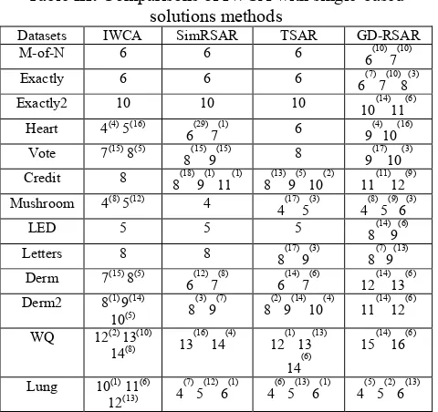
IWCA is contrasted with other attribute reduction methods which have been investigated. The best reduct that is obtained out of 20 runs for each method is recorded, and the number of runs which achieved this reduct has been stated in parentheses. Where a number appears without a superscript it indicates that this method managed to obtain the number of attributes for all the runs.

The contrasted methods are categorised into single-based solution and population-based solution methods. Table III gives a comparison of the results of this study with single-based solution methods (e.g. Simulated Annealing (SimRSAR) [1], Tabu Search (TSAR) [9], Great Deluge algorithm (GD-RSAR) [7].

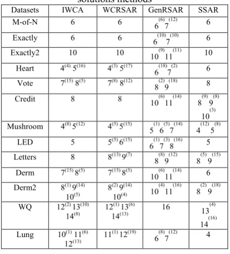
Table VI gives a comparison between the results of this study with population-based solutions methods (e.g. Genetic Algorithm (GenRSAR) [1,14], Scatter Search (SSAR) [16]). From the results given in Table III, the proposed method is comparable with the available single based methods, it can be seen that IWCA produced better results than SimRSAR, IS-CNS and in 4 datasets, i.e. heart, vote credit and wq. IWCA outperforms TSAR in 5 datasets i.e. heart, vote credit, led and wq. However IWCA has outperforms GD-RSAR in 12 datasets, i.e. m-of-n, exactly, exactly2, heart, vote, credit, mushroom, led, letters, derm, derm2 and wq. Table VI shows the comparison between the proposed method IWCA and the available population-based approaches in the literature. The results reported show that the performance of IWCA is significantly better than the performance of WCARSAR in 6 datasets, i.e. heart, vote, led, letters, wq and lung. However IWCA has outperforms GenRSAR in 12 datasets, i.e. m-of-n, exactly, exactly2, heart, vote, credit, mushroom, led, letters, derm, derm2 and wq. IWCA outperforms SSAR in 6 datasets i.e. heart, vote, credit, mushroom, letters and wq.

V. CONCLUSION AND FUTURE WORK In conclusion, The IWCA has been tested on the public domain datasets that are available in UCI. From the results it can be seen that the proposed method IWCA better than other methods of attribute selection. This indicates that the IWCA better than the current methods in data mining optimization. In this paper, we improve the basic algorithm with the local search algorithm by Hybridizing Water Cycle Algorithm with Hill Climbing Algorithm in order to improve the exploitation process of the WCA. Our future works to hybrid the proposed method with other population and local search algorithms. The proposed methods presented in this paper can be applied on other real world problem domains that arise in data mining research field such as clustering, text mining, bioinformatics and speech recognition, which may yield interesting results.

Table III: Comparisons of IWCA with single-based

solutions methods

Datasets IWCA SimRSAR TSAR GD-RSAR

M-of-N 6 6 6 ₆(10)

7(10)

Exactly 6 6 6 ₆(7)

7(10)8(3)

Exactly2 10 10 10 ₁₀(14)

11(6) Heart 4(4) ₅(16)

6(29) 7(1) 6 9(4)10(16)

Vote 7(15) ₈(5)

8(15) 9(15) 8 9(17)10(3)

Credit 8 ₈(18)

9(1) 11(1) 8(13) 9(5) 10(2) 11(11)12(9) Mushroom 4(8) ₅(12) ₄

4(17) 5(3) 4(8) 5(9)6(3)

LED 5 5 5 ₈(14)

9(6)

Letters 8 8 ₈(17)

9(3) 8(7)9(13) Derm 7(15) ₈(5)

6(12) 7(8) 6(14) 7(6) 12(14)13(6) Derm2 8(1) ₉(14)

10(5) 8 (3)

9(7) 8(2) 9(14) 10(4) 11(14)12(6)

WQ 12(2) ₁₃(10)

14(8) 13 (16)

14(4) 12(1) 13(13) 14(6)

15(14)16(6)

Lung 10(1) ₁₁(6)

12(13) 4

(7)

Table VI: Comparisons of IWCA with population-based solutions methods

Datasets IWCA WCRSAR GenRSAR SSAR

M-of-N 6 6 ₆(6)

7(12) 6

Exactly 6 6 ₆(10)

7(10) 6

Exactly2 10 10 ₁₀(9)

11(11) 10 Heart 4(4) ₅(16) ₄(3) ₅(17)

6(18)7(2) 6 Vote 7(15) ₈(5) ₇(8) ₈(12)

8(2)9(18) 8

Credit 8 8 ₁₀(6)

11(14) 8(9) 9(8) 10(3) Mushroom 4(8) ₅(12) ₄(5) ₅(15)

5(1)6(5)7(14) 4(12) 5(8)

LED 5 5(5) ₆(15)

6(1)7(3)8(16) 5 Letters 8 8(13) ₉(7)

8(8)9(12) 8(5) 9(15) Derm 7(15) ₈(5) ₇(15) ₈(5)

10(6)11(14) 6 Derm2 8(1) ₉(14)

10(5) 8 (2) ₉(14) 10(4) 10

(4)

11(16) 8(2) 9(18)

WQ 12(2) ₁₃(10)

14(8) 12 (1) ₁₃(6)

14(13) 16 13

(4)

14(16) Lung 10(1) ₁₁(6)

12(13) 11

(1) ₁₂(19)

6(8)7(12) 4

REFERENCE

[1] R. Jensen and Q. Shen, "Semantics-Preserving Dimensionality Reduction: Rough and Fuzzy-Rough-Based Approaches," IEEE Trans. on Knowl. and Data Eng., vol. 16, pp. 1457-1471, 2004.

[2] A. Skowron and C. Rauszer, "The discernibility matrices and functions in information systems," Intelligent decision support–Handbook of applications and advances of the rough set theory, pp. 311–362, 1992.

[3] H. Liu and H. Motoda, Feature Selection for Knowledge Discovery and Data Mining. Boston: Kluwer Academic Publishers 1998.

[4] I. Guyon and A. Elisseeff, "An introduction to variable and feature selection," The Journal of Machine Learning Research, vol. 3, pp. 1157-1182, 2003. [5] Mafarja, Majdi, and Salwani Abdullah.

"Record-To-Record Travel Algorithm For Attribute Reduction In Rough Set Theory." Journal of Theoretical and Applied Information Technology 49.2 (2013).

[6] F. Glover and G. Kochenberger, Handbook of Metaheuristics (International Series in Operations Research & Management Science): Springer, 2003. [7] Z. Pawlak, Rough Sets: Theoretical Aspects of Reasoning about Data: Kluwer Academic Publishers, 1991.

[7] Abdullah, Salwani, and Najmeh Sadat Jaddi. "Great Deluge Algorithm for Rough Set Attribute Reduction." Database Theory and Application, Bio-Science and Bio-Technology. Springer Berlin Heidelberg, 2010. 189-197.

[8] Jihad, SaifKifah, and S. Abdullah."Investigating composite neighbourhood structure for attribute reduction in rough set theory." Intelligent Systems Design and Applications (ISDA), 2010 10th International Conference on. IEEE, 2010.

[9] Hedar, Abdel-Rahman, Jue Wang, and Masao Fukushima. "Tabu search for attribute reduction in

rough set theory." Soft Computing 12.9 (2008): 909-918.

[10] Abdullah, Salwani, et al. "A constructive hyper-heuristics for rough set attribute reduction." Intelligent Systems Design and Applications (ISDA), 2010 10th International Conference on. IEEE, 2010.

[11] Arajy, Yahya Z., and Salwani Abdullah. "Hybrid variable neighbourhood search algorithm for attribute reduction in Rough Set Theory." Intelligent Systems Design and Applications (ISDA), 2010 10th International Conference on. IEEE, 2010.

[12] Mafarja, Majdi, and Salwani Abdullah. "Modified great deluge for attribute reduction in rough set theory." Fuzzy Systems and Knowledge Discovery (FSKD), 2011 Eighth International Conference on. Vol. 3. IEEE, 2011.

[13] Jaddi, Najmeh Sadat, and Salwani Abdullah. "Nonlinear Great Deluge Algorithm for Rough Set Attribute Reduction." Journal of Information Science and Engineering 29.1 (2013): 49-62.

[14] Jensen, Richard, and Qiang Shen. "Finding rough set reducts with ant colony optimization." Proceedings of the 2003 UK workshop on computational intelligence. Vol. 1. No. 2. 2003.

[15] Ke, Liangjun, Zuren Feng, and Zhigang Ren. "An efficient ant colony optimization approach to attribute reduction in rough set theory." Pattern Recognition Letters 29.9 (2008): 1351-1357.

[16] Wang, Jue, et al. "Scatter search for rough set attribute reduction."Computational Sciences and Optimization, 2009. CSO 2009. International Joint Conference on. Vol. 1. IEEE, 2009.

[17] Z. Pawlak, A. Skowron. Rough membership functions. In R. Yager, M. Fedrizzi, J. Kacprzyk (eds.), Advances in the Dempster-Shafer Theory of Evidence, Wiley, New York, pp 251-271. 1994

[18] A. Chouchoulas and Q. Shen. Rough set-aided keyword reduction for text categorisation. Applied Artificial Intelligence, 15(9):843-873, 2001.

[19] Eskandar, Hadi, et al. "Water cycle algorithm–A novel metaheuristic optimization method for solving constrained engineering optimization problems." Computers & Structures (2012).