Abstract—Some complex natural phenomena in physics,
economics and engineering can be represented by Integral Equations (IE). But one may be short of general mathematical tricks to solve them analytically, which could quickly turn into a life time enterprise. In the contrary, the use of computers or numerical methods introduced some decades ago has brought a different approach that is innovative and effective.
In addition, the theory of measure, the study of polynomials and normed spaces, namely Banach, Hilbert, Lebesgue, Hölder, Lipschitz and Sobolev spaces led to advanced modern numerical methods to solve these complex IEs. When using computer, a generally continuous domain is divided into smaller pieces, or elements, so the calculation on any point of the continuous domain could be done using results from the elements; it is similar to approximate a circle by a regular polygon; as the number of side increases, the polygon become more and more close to a circle.
This method of solving IEs using subdivisions of the domain, along with discrete form of the equations, is referred to as the Finite Element Method (FEM). In this paper, we implement the advanced core theory of the finite element method into adaptive meshes for generic complex problems represented by IEs.
Index Terms—Finite Element, Integral Equation,
Interpolation Operator, Adaptive Mesh.
I. INTRODUCTION
HIS paper covers the implementation of the FEM that we have developed from scratch, which helped us fully extend our understanding of the topic and program the actual computer codes in solving IEs and be able to compare various approximation methods. This paper is organized into three main parts.
The first part summarizes the theoretical foundation of the FEM as well as an overview of the Finite Element interpolation technique. It restates the results on normed vector spaces ([1], p.463-492; [3], p.13-17; [4]), Lebesgue integration, distributional derivatives and Sobolev spaces ([1], p.463-492; [3], p.13-17), essential to derive “error estimate”, convergence and well posedness.
Next, we review Integral Equations ([2], p.222-337; [3], p.31-42) and their approximation methods and results.
The last part, Implementation, covers practical implementation considerations such as meshing techniques, “a posterior error estimate” for mesh refinement or adaptive mesh ([1], p.337-457; [3], p.68-112), examples illustrating our simulator results.
Manuscript received September 29, 2014; revised Jan 02, 2015. D.N.Ovono is an oil & gas engineer and researcher, he works for Halliburton, phone: 1-832-706-4036
(e-mail:[email protected]).
II. THEORETICALFOUNDATIONSOFTHEFINITE
ELEMENTMETHOD
A. Theoretical Framework and Fundamental Analysis Please refer to ([1], p.463-492; [3], p.13-17) for a complete overview.
Lebesgue Spaces: 𝐿1() is the space of the scalar-valued functions that are Lebesgue-integrable. The space of locally integrable functions is denoted by 𝐿1𝑙𝑜𝑐() and is defined as 𝐿1𝑙𝑜𝑐() = {𝑓 ∈ 𝑀(); ∀ 𝑐𝑜𝑚𝑝𝑎𝑐𝑡 𝐾 ⊂, 𝑓 ∈ 𝐿1(𝐾)}
For 1 ≤ 𝑝 ≤ +∞, let 𝐿𝑝() = {𝑓 ∈ 𝑀(); ‖𝑓‖0,𝑝,<
+∞} where
‖𝑓‖0,𝑝,= (∫ |𝑓(𝑥)|𝑝
)
1 𝑝
𝑑𝑥, 𝑓𝑜𝑟 1 ≤ 𝑝 ≤ +∞ ‖𝑓‖0,∞,= 𝑒𝑠𝑠 sup|𝑓(𝑥)| = inf {𝑀 ≥ 0; |𝑓(𝑥)| ≤ 𝑀, 𝑓 ∈
Sobolev Spaces: Let 𝑠 and 𝑝 be two integers with 𝑠 ≥ 0 and
1 ≤ 𝑝 ≤ +∞, the Sobolev space is defined as
𝑊𝑠,𝑝() = {𝑢 ∈ 𝐷′(); ∂𝛼𝑢 ∈ 𝐿𝑝(), |𝛼| ≤ 𝑠}
with distributional derivatives ([1], p.463-492). There follows that 𝑊𝑠,𝑝() is a Banach space when equipped with the norm
‖𝑢‖𝑊𝑠,𝑝()= ∑ ‖∂𝛼𝑢‖𝐿𝑝() |𝛼|≤𝑠
For 𝑝 = 2, 𝑊𝑠,2() has an Hilbert structure and is denoted by 𝐻𝑠().
B. Overview of the Finite Element Interpolation
Please refer to ([1], p.3-58; [3], p.18-25) for a complete literature.
Polynomials Used for One-Dimensional Interpolation: The mesh: a mesh of = ]𝑎, 𝑏[ is an indexed collection of intervals with non-zero measure {𝐼𝑖= [𝑥𝑖, 𝑥𝑖+1]}0≤𝑖≤𝑁
forming a partition of , ie, ̅ = ⋃ 𝐼𝑁𝑖=0 𝑖 and 𝐼𝑖∩ 𝐼𝑗≠ ∅ for
𝑖 ≠ 𝑗. It is constructed by taking 𝑁 + 2 points of ̅ such that
𝑎 = 𝑥0< 𝑥1< ⋯ < 𝑥𝑁< 𝑥𝑁+1= 𝑏. The mesh is denoted
by T h= {𝐼𝑖}0≤𝑖≤𝑁, where ℎ𝑖= 𝑥𝑖+1− 𝑥𝑖 may be a variable
step size and the subscript ℎ = max0≤𝑥≤𝑁ℎ𝑖 refers to a
refinement. The points in the set {𝑥0, … , 𝑥𝑁+1} are called the vertices of the mesh and the intervals 𝐼𝑖 are referred to as elements or cells.
The ℙ𝑘 Lagrange finite element: Let 𝑘 ≥ 1 and let {𝑠0, … , 𝑠𝑘} be 𝑘 + 1 distinct numbers. The Lagrange polynomials {ℒ0𝑘, … , ℒ𝑘𝑘} associated with the nodes
{𝑠0, … , 𝑠𝑘} are defined to be ℒ𝑚𝑘(𝑡) =∏∏𝑙≠𝑚(𝑠(𝑡−𝑠𝑙) 𝑚−𝑠𝑙)
𝑙≠𝑚 , 0 ≤ 𝑚 ≤
𝑘 and satisfy the important propriety ℒ𝑚𝑘(𝑠𝑙) = 𝛿𝑚𝑙, 0 ≤ 𝑚, 𝑙 ≤ 𝑘. For 𝑗 ∈ {0, … , 𝑘(𝑁 + 1)} with 𝑗 = 𝑘𝑖 + 𝑚 and 0 ≤ 𝑚 ≤ 𝑘 − 1, define the functions
𝜑𝑘𝑖+𝑚(𝑥) = { ℒ𝑖,𝑚
𝑘 (𝑥) 𝑖𝑓 𝑥 ∈ 𝐼 𝑖 0 𝑜𝑡ℎ𝑒𝑟𝑤𝑖𝑠𝑒
Finite Element Solution to Integral Equations
Dieudonne Ndong Ovono
and for 𝑚 = 0 𝜑𝑘𝑖(𝑥) = {
ℒ𝑖−1,𝑘𝑘 (𝑥) 𝑖𝑓 𝑥 ∈ 𝐼𝑖−1 ℒ𝑖,0𝑘 (𝑥) 𝑖𝑓 𝑥 ∈ 𝐼𝑖 0 𝑡ℎ𝑒𝑟𝑤𝑖𝑠𝑒
On 𝐼𝑖= [𝑥𝑖, 𝑥𝑖+1] ∈ T h let choose the local degrees of
freedom to be the (k+1) linear forms 𝑖= {𝜎𝑖,0, … , 𝜎𝑖,𝑘}
defined by 𝜎𝑖,𝑚: ℙ𝑘∋ 𝑝 ⟼ 𝜎𝑖,𝑚(𝑝) = 𝑝(𝑖,𝑚), 0 ≤ 𝑚 ≤ 𝑘 for all 𝑝 ∈ ℙ𝑘. 𝑖 is a basis of ℒ(ℙ𝑘, ℝ) and the triplet
{𝐼𝑖, ℙ𝑘,𝑖} is called a one-dimensional ℙ𝑘 Lagrange finite element. the nodes are {𝑖,0, … ,𝑖,𝑘}; the local shape functions at nodes are the (k+1) Lagrange polynomials ℒ𝑖,𝑚𝑘 ,
0 ≤ 𝑚 ≤ 𝑘.
Types of Finite Elements: Definitions and Examples
Main definition: following Ciarlet, a finite element is defined as a triplet {𝐾, 𝑃,} where:
(i) 𝐾 is a compact, connected, Lipschitz subset of ℝ𝑑with non-empty interior.
(ii)𝑃 is a vector space of functions 𝑝: 𝐾 ⟼ ℝ𝑚 for some positive integer 𝑚, typically 𝑚 = 1 or d.
(iii) is a set of 𝑛𝑠ℎ linear forms = {𝜎1, … , 𝜎𝑛𝑠ℎ}, called local degrees of freedom, acting on the elements of 𝑃,
and such that the linear mapping
𝑃 ∋ 𝑝 ⟼ (𝜎1(𝑝), … , 𝜎𝑛𝑠ℎ(𝑝)) , 𝜎𝑖,𝑚(𝑝) ∈ ℝ𝑛𝑠ℎis
bijective, i.e., is a basis for ℒ(𝑃; ℝ).
Then, there exists a basis {𝜃1, … , 𝜃𝑛𝑠ℎ} in 𝑃, called the local shape functions, such that 𝜎𝑖(𝜃𝑗) = 𝑝(𝜃𝑗), 1 ≤ 𝑖, 𝑗 ≤ 𝑛𝑠ℎ;
dim 𝑃 = 𝑐𝑎𝑟𝑑 = 𝑛𝑠ℎ and ∀𝑝 ∈ 𝑃, (𝜎𝑖(𝑝) = 0, 1 ≤ 𝑖 ≤ 𝑛𝑠ℎ) ⇒ (𝑝 = 0), this propriety is known as unisolvence.
Lagrange finite element: For all 𝑝 ∈ 𝑃, 𝜎𝑖(𝑝) = 𝑝(𝑎𝑖), 1 ≤ 𝑖 ≤ 𝑛𝑠ℎ, {𝐾, 𝑃,} is called a Lagrange finite element. The
local shape functions {𝜃1, … , 𝜃𝑛𝑠ℎ}, with 𝜃𝑖(𝑎𝑗) = 𝛿𝑖𝑗, 1 ≤
𝑖, 𝑗 ≤ 𝑛𝑠ℎ, are called the nodal basis of 𝑃.
Simplicial Lagrange finite element: Let {𝑎0, … , 𝑎𝑑} be a
family of points in ℝ𝑑, 𝑑 ≥ 1. Assume that the vector
{𝑎1− 𝑎0, … , 𝑎𝑑− 𝑎0} are linearly independent. Then, the
convex hull of {𝑎0, … , 𝑎𝑑} is called a simplex, and the points {𝑎0, … , 𝑎𝑑} are called the vertices of the simplex. Let ℙ𝑘 be
the space of polynomials in the variables 𝑥1, … , 𝑥𝑑, with real
coefficient and global degree at most 𝑘:
ℙ𝑘 = {𝑝(𝑥) = ∑ 𝛼𝑖1…𝑖𝑑𝑥1𝑖1… 𝑥𝑑 𝑖𝑑 0≤𝑖1,…,𝑖𝑑≤𝑘
𝑖1+⋯+𝑖𝑑≤𝑘
; 𝛼𝑖1…𝑖𝑑 ∈ ℝ}, ℙ𝑘 is a vector space of dim ℙ𝑘 = (𝑑+𝑘𝑘 )
There is also “Tensor Product” and “Prismatic” finite elements where the shape of cell is a cuboid, respectively a prism.
The Crouzeix-Raviart finite element:
𝑃 = ℙ1 and take for the local degrees of freedom the mean-value over the (𝑑 + 1) faces of 𝐾, i.e., for 0 ≤ 𝑖 ≤ 𝑑,
𝜎𝑖(𝑝) =𝑚𝑒𝑎𝑠(𝐹1
𝑖)∫ 𝑝𝐹𝑖 . Let ={𝜎𝑖}0≤𝑖≤𝑑, then {𝐾, ℙ1,} is a
finite element. The local shape functions are 𝜃𝑖(𝑥) = 𝑑(1𝑑− 𝜆𝑖(𝑥)), 0 ≤ 𝑖 ≤ 𝑑. The local Crouzeix-Raviart interpolation
operator is then defined as follows 𝔗𝑘𝐶𝑅: 𝑉(𝐾) ∋ 𝑣 ⟼ 𝔗𝑘𝐶𝑅𝑣 = ∑ (𝑚𝑒𝑎𝑠(𝐹1
𝑖)∫ 𝑣𝐹𝑖 ) 𝜃𝑖 𝑑
𝑖=0 ∈ ℙ1
Other finite element type are Raviart-Thomas, Nedelec, Hermite, etc.
Meshes: Basic Concepts
Mesh: Let be a domain in ℝ𝑑. A mesh is a union of a finite number 𝑁𝑒𝑙 of compact, connected, Lipschitz sets 𝐾𝑚,
called mesh cells or elements, with non-empty interior such that {𝐾𝑚}1≤𝑚≤𝑁𝑒𝑙 form a partition of , i.e.,
̅ = ⋃𝑁𝑚=1𝑒𝑙 𝐾𝑚 and 𝐾𝑚∩ 𝐾𝑛≠ ∅ for 𝑚 ≠ 𝑛. A mesh {𝐾𝑚}1≤𝑚≤𝑁𝑒𝑙 is denoted by 𝔗ℎ, ℎ referring to the refinement
level so that
∀𝐾 ∈ 𝔗ℎ, ℎk= 𝑑𝑖𝑎𝑚(𝐾) = max𝑥1,𝑥2∈𝐾‖𝑥1− 𝑥2‖𝑑, where ‖. ‖𝑑 is the Euclidian norm in ℝ𝑑 and ℎ = max𝐾∈𝔗ℎℎk
A sequence of successive refinement meshes is denoted by
{𝔗ℎ}ℎ>0.
Mesh generation: In practice, the mesh is generated from a reference cell 𝐾̂, and a set of geometric transformations mapping 𝐾̂ to the actual mesh cells 𝐾 ∈ 𝔗ℎ, denote by 𝑇ℎ: 𝐾̂ → 𝐾. We shall henceforth assume that the geometric
transformations are C1-diffeomorphisms. Usually 𝑇ℎis specified using the Lagrange finite element {𝐾,̂ 𝑃̂𝑔𝑒𝑜,̂𝑔𝑒𝑜},
called the geometric reference finite element. Let 𝑛𝑔𝑒𝑜=
𝑐𝑎𝑟𝑑(̂𝑔𝑒𝑜), {𝑔̂1, … , 𝑔̂𝑛𝑔𝑒𝑜} referred to as the geometric reference nodes of 𝐾̂ associated with ̂𝑔𝑒𝑜 and
{̂1, … ,̂𝑛𝑔𝑒𝑜} are the geometric reference shape functions. When 𝐾̂ is a simplex, 𝔗ℎ is called a simplicial mesh. A mesh generator usually provides a list of 𝑛𝑔𝑒𝑜-uplets {𝑔̂1𝑚, … , 𝑔̂𝑛𝑚𝑔𝑒𝑜}1≤𝑚≤𝑁𝑒𝑙, called geometric nodes of the m
th
element, where 𝑔𝑖𝑚∈ ℝ𝑑 and 𝑁𝑒𝑙 is the number of mesh
elements. The geometric transformations are 𝑇𝑚: 𝐾̂ ∋ 𝑥̂ ⟼ 𝑇𝑚(𝑥̂) = ∑ 𝑔𝑖𝑚
𝑛𝑔𝑒𝑜
𝑖=1 ̂𝑖(𝑥̂) ∈ ℝ𝑑 so that 𝑇𝑚(𝑔̂𝑖) = 𝑔𝑖𝑚 for 1 ≤ 𝑖 ≤ 𝑛𝑔𝑒𝑜 and 𝐾𝑚= 𝑇𝑚(𝐾̂). The numbering of the
nodes had to be compatible, henceforth the convention that the Jacobian of 𝑇𝑚 be positive so that 𝑇𝑚 is a C1 -diffeomorphisms. When the transformation is affine, the mesh is called an affine mesh and if 𝐾̂ is a simplex, the affine mesh is called a triangulation. For domain with a curved boundary, the mesh is generated using geometric transformation of degree 𝑘𝑔𝑒𝑜> 1.
Approximation Spaces and Interpolation Operators Global interpolation operator: A global interpolation operator can be constructed by first choosing its domain to be
𝐷(𝔗ℎ) = {𝑣 ∈ [𝐿1(ℎ)]𝑚; ∀𝐾 ∈ 𝔗ℎ, 𝑣|𝐾∈ 𝑉(𝐾)}, then
the global interpolation operator 𝔗ℎ𝑣 is defined
elementwise, using the local interpolation operator, by
𝔗ℎ: 𝐷(𝔗ℎ) ∋ 𝑣 ⟼ ∑𝐾∈𝔗ℎ∑𝑛𝑖=1𝑠ℎ𝜎𝐾,𝑖(𝑣|𝐾)𝜃𝐾,𝑖∈ 𝑊ℎ, where
the so called approximation space 𝑊ℎ = {𝑣ℎ∈ [𝐿1(
ℎ)]𝑚; ∀𝐾 ∈ 𝔗ℎ, 𝑣|𝐾∈ 𝑃𝐾} is the codomain of 𝔗ℎ. If 𝑊ℎ⊂ 𝑉, where 𝑉 is a Banach space, 𝑊ℎis said to be V-conformal.
III. APPROXIMATIONOFINTEGRALEQUATIONS Please, refer to ([2], p.222-337) for an in depth overview on integral equations or ([3], p.31-42) for summary.
A.
Introductionare involved. The most frequent form is the Fredholm equation:
𝛼(𝑥)𝑦(𝑥) = 𝐹(𝑥) +∫ 𝐾(𝑥, 𝜀)𝑦(𝜀)𝑑𝜀 𝑏
𝑎
If 𝑏 = 𝑥 is identified with the current variable, the equation is known as the Volterra equation. , 𝑎 𝑎𝑛𝑑 𝑏 are constants and
𝛼, 𝐹 and 𝐾are given functions, continuous on (𝑎, 𝑏) as well as 𝑦(𝑥). 𝐾(𝑥, 𝜀) is known as the kernel. The integral equation is said to be of the first kind if 𝛼 ≡ 0, second kind if 𝛼 ≡ 1 and of the third kind if 𝛼 is a function. If 𝛼 is positive, the Fredholm equation can take the form
√𝛼(𝑥)𝑦(𝑥) = 𝐹(𝑥)
√𝛼(𝑥)+∫
𝐾(𝑥, 𝜀)
√𝛼(𝑥)𝛼(𝜀)√𝛼(𝜀)𝑦(𝜀)𝑑𝜀 𝑏
𝑎
and be considered of the second kind in the unknown function √𝛼(𝑥)𝑦(𝑥) with a modified kernel. For a two-dimensional variable 𝑤(𝑥, 𝑦), the Fredholm equation is of the form
𝛼(𝑥, 𝑦)𝑤(𝑥, 𝑦) = 𝐹(𝑥, 𝑦) +∬ 𝐾(𝑥, 𝑦; 𝜀, )𝑤(𝜀,)𝑑𝜀𝑑
B.
Numerical Solution of Integral EquationsApproximation of Fredholm Equations by Sets of Algebraic Equations:
A definite integral of the form 𝐽 = ∫ 𝑓(𝜀)𝑑𝜀𝑎𝑏 can be defined as a limit of the form 𝐽 = lim
𝑛 → ∞∑𝑛𝑘=1𝑓(𝑥𝑘)(𝑥)𝑘where the
interval (𝑎, 𝑏) is divided in subintervals of length (𝑥)𝑘 and 𝑥𝑘 is the point of the 𝑘𝑡ℎ interval. The integral "𝐽" can be
obtained by not proceeding to the limit but using a weighting coefficient 𝐷𝑘 at 𝑥𝑘 so that 𝐽 = ∑𝑛𝑘=1𝐷𝑘𝑓(𝑥𝑘). 𝐷𝑘 can be (𝑥)𝑘 or in accordance with some rule such as the trapezoidal rule{𝐷1, 𝐷2, … , 𝐷𝑛−1, 𝐷𝑛} = ℎ{12, 1,1, … ,1,1,12} or
the Simpson’s rule{𝐷1, 𝐷2, 𝐷3, 𝐷4… , 𝐷𝑛−3, 𝐷𝑛−2, 𝐷𝑛−1, 𝐷𝑛} = ℎ
3{1,4,2,4 … ,4,2,4,1} where ℎ = (𝑏 − 𝑎)/(𝑛 − 1). There
follows that the solution of
𝑦(𝑥) = 𝐹(𝑥) +∫ 𝐾(𝑥, 𝜀)𝑦(𝜀)𝑑𝜀𝑎𝑏 is approximated by
𝑦(𝑥𝑖) = 𝐹(𝑥𝑖) +∑𝑛𝑘=1𝐷𝑘𝐾(𝑥𝑖, 𝑥𝑘)𝑦(𝑥𝑘) or 𝑦𝑖= 𝑓𝑖+
∑𝑛𝑘=1𝐾𝑖𝑘𝐷𝑘𝑦𝑘. If 𝑦 = {𝑦𝑖}, 𝐾 = [𝐾𝑖𝑗], 𝐷 = [𝐷𝑖𝛿𝑖𝑗] and 𝑓 = {𝑓𝑖}, thus (𝐼 −𝐾𝐷)𝑦 = 𝑓 where 𝐼 is the unit matrix of
order n. This method is particularly useful when the kernel 𝐾 is available as a table of values of an empirical influence function. In the other hand, the characteristic numbers of
𝑦(𝑥) =∫ 𝐾(𝑥, 𝜀)𝑦(𝜀)𝑑𝜀𝑎𝑏 are afforded by reciprocals of the characteristic numbers of the corresponding matrix formulation 𝑦 =∑𝑛𝑘=1𝐾𝑖𝑘𝐷𝑘𝑦𝑘 =𝐾𝐷𝑦.
Approximation Methods of Undetermined Coefficients In this method the solution of
𝑦(𝑥) = 𝐹(𝑥) +∫ 𝐾(𝑥, 𝜀)𝑦(𝜀)𝑑𝜀𝑎𝑏 is approximated by
𝑦(𝑥)∑𝑛𝑘=1𝑐𝑘𝑘(𝑥) leading to the form ∑𝑛𝑘=1𝑐𝑘[𝑘(𝑥)−𝑘(𝑥)]𝐹(𝑥) where
𝑘(𝑥) = ∫ 𝐾(𝑥, 𝜀)𝑘(𝜀)𝑑𝜀 𝑏
𝑎 (𝑎 ≤ 𝑥 ≤ 𝑏) and the 𝑘are
suitably chosen functions such as 𝑥𝑘 and the c’s are determined by a set of n algebraic equations. If end values are known in advance, it may be desirable to use
𝑦(𝑥)0(𝑥) + ∑𝑛𝑘=1𝑐𝑘𝑘(𝑥), with 0(𝑥) verifying the
known end conditions and the remaining ‘s vanishing at end points.
The Method of Collocation
Following the preceding section by setting 𝑠𝑘(𝑥) =𝑘(𝑥) −
𝑘(𝑥) ≡𝑘(𝑥) −∫ 𝐾(𝑥, 𝜀)𝑎𝑏 𝑘(𝜀)𝑑𝜀 (𝑎 ≤ 𝑥 ≤ 𝑏) and
by requiring that ∑𝑛𝑘=1𝑐𝑘𝑠𝑘(𝑥)𝐹(𝑥) be an equality at n distinct points in (𝑎, 𝑏), we obtain the n conditions
∑𝑛𝑘=1𝑐𝑘𝑠𝑘(𝑥𝑖)= 𝐹(𝑥𝑖) or 𝑆𝑐 = 𝑓 where
𝑐 = {𝑐𝑖}, 𝑆 = [𝑠𝑖𝑗] with 𝑠𝑖𝑗 = 𝑠𝑖(𝑥𝑗) and 𝑓 = {𝑓𝑖} (i=1, 2, …,n), leading to the n algebraic equations in 𝑐𝑘, hence 𝑦(𝑥). The Method of Weighting Functions or Galerkin
This method uses the n orthogonality conditions of the form
∑ 𝑐𝑘∫ 𝑖𝑠𝑘𝑑𝑥 = ∫ 𝑖𝐹𝑑𝑥 (𝑖 = 1, 2, … , 𝑛) 𝑏
𝑎 𝑏
𝑎 𝑛
𝑘=1 or 𝑀𝑐 = 𝑏
where 𝑀 = [𝑚𝑖𝑗] with 𝑚𝑖𝑗= ∫𝑎𝑏𝑖𝑠𝑗𝑑𝑥 and 𝑏𝑖= ∫𝑎𝑏𝑖𝐹𝑑𝑥 (𝑖 = 1, 2, … , 𝑛); a convenient choice of 𝑖 is
1, 𝑥, 𝑥2, … , 𝑥𝑛; it is desirable to choose the
𝑖 as a complete
set of functions. The system 𝑀𝑐 = 𝑏 leads to n algebraic equations in 𝑐𝑘, hence 𝑦(𝑥).
The Method of Least Square
This method requires that the integral of the square of the difference ∑𝑛𝑘=1𝑐𝑘𝑠𝑘(𝑥)− 𝐹(𝑥) be as small as possible or
∫ [∑𝑎𝑏 𝑛𝑘=1𝑐𝑘𝑠𝑘(𝑥)− 𝐹(𝑥)]2𝑑𝑥=minimum and avoids the
dependence on the choice of the collocation points or weighting functions. There then follows that
∫ 𝑠𝑎𝑏 𝑖(𝑥)[∑𝑛𝑘=1𝑐𝑘𝑠𝑘(𝑥)− 𝐹(𝑥)]𝑑𝑥 = 0 or ∑𝑛𝑘=1𝑐𝑘∫ 𝑠𝑎𝑏 𝑖𝑠𝑘𝑑𝑥 = ∫ 𝑠𝑎𝑏 𝑖𝐹𝑑𝑥 (𝑖 = 1, 2, … , 𝑛) leading to ∑𝑛𝑘=1𝑐𝑘[∑𝑟=1𝑁 𝐷𝑟𝑠𝑖(𝑥𝑟)𝑠𝑘(𝑥𝑟)] = ∑𝑟=1𝑁 𝐷𝑟𝑠𝑖(𝑥𝑟)𝐹(𝑥𝑟) (𝑖 = 1, 2, … , 𝑛) or ∑𝑛𝑘=1𝑐𝑘𝑝𝑖𝑘 =𝑞𝑖, with change in indices, we obtain
with 𝑃 = [𝑝𝑖𝑗]= ∑𝑁𝑟=1𝐷𝑟𝑠𝑖(𝑥𝑟)𝑠𝑘(𝑥𝑟)= ∑𝑁𝑘=1𝑠𝑘𝑖𝐷𝑘𝑠𝑘𝑗= 𝑆𝑇𝐷𝑆 and 𝑞 = {𝑞
𝑖}= ∑𝑁𝑘=1𝑠𝑘𝑖𝐷𝑘𝑓𝑖= 𝑆𝑇𝐷𝑓 where 𝑆 = [𝑠𝑖𝑗] ≡ [𝑠𝑖(𝑥𝑗)], 𝐷 = [𝐷𝑖𝛿𝑖𝑗], and 𝑓 = {𝑓𝑖}.
Since 𝐷 is diagonal, 𝑆𝑇𝐷 = (𝐷𝑆)𝑇, 𝑃 = (𝐷𝑆)𝑇𝑆 and
𝑞 = (𝐷𝑆)𝑇𝑓, this result leads to the following procedure for
determining the n linear equations represented by
∑𝑛𝑘=1𝑐𝑘𝑠𝑘(𝑥𝑖)= 𝐹(𝑥𝑖) 1) Choose 𝑁 points in (𝑎, 𝑏) and
write down the 𝑁 equations. 2) Denote by 𝑆 the 𝑁 𝑥 𝑛 matrix of coefficients in the previous set of equations and form the “weighting matrix” 𝑆∗=DS
by multiplying the ith row of S by the weighting coefficient 𝐷𝑖
associated with the point 𝑥𝑖 in an appropriate integration
scheme involving the 𝑁 points. 3) Pre-multiply the augmented matrix of ∑𝑛𝑘=1𝑐𝑘𝑠𝑘(𝑥𝑖)= 𝐹(𝑥𝑖) (𝑖 =
1, 2, … , 𝑁) by the transpose of the weighting matrix 𝑆∗. The resultant matrix is the augmented matrix of the required set of n linear equations which determines the constants
𝑐1, 𝑐2, … , 𝑐𝑛.
Approximation of the Kernel
It is sometimes convenient to approximate a kernel by a polynomial in 𝑥 and 𝜀 or by a separable kernel and solve the resultant equation according to the method of separable kernel. For instance, a kernel can be approximated by
𝐴1+ 𝐴2𝑥 + 𝐴3𝑥2 or 𝑥(1 − 𝑥)(𝐵1+ 𝐵2𝑥 + 𝐵3𝑥2) which
C.
Application: Comparison of Collocation, Galerkin, Least Square and Kernel ApproximationCompare the exact solution of the following integral equation, if it exists, with approximate solutions from the methods of collocation, Galerkin, least square and kernel approximation:
𝑦(𝑥) = 𝑥 + ∫ 𝐾(𝑥, 𝜀)𝑦(𝜀)𝑑𝜀01 where 𝐾(𝑥, 𝜀) =
{𝑥, when x < 𝜀 𝜀, when x > 𝜀
a) Exact solution:
By writing ∫ 𝐾(𝑥, 𝜀)𝑦(𝜀)𝑑𝜀01 = ∫ 𝐾(𝑥, 𝜀)𝑦(𝜀)𝑑𝜀0𝑥 +
∫ 𝐾(𝑥, 𝜀)𝑦(𝜀)𝑑𝜀𝑥1 =∫ 𝜀𝑦(𝜀)𝑑𝜀0𝑥 + ∫ 𝑥𝑦(𝜀)𝑑𝜀𝑥1 and by using the relation
𝑑
𝑑𝑥∫ 𝐺(𝑥, 𝜀)𝑑𝜀
𝐵(𝑥)
𝐴(𝑥) = ∫
𝜕𝐺(𝑥,𝜀) 𝜕𝑥 𝐵(𝑥)
𝐴(𝑥) 𝑑𝜀 + 𝐺[𝑥, 𝐵(𝑥)]
𝑑𝐵(𝑥)
𝑑𝑥 −
𝐺[𝑥, 𝐴(𝑥)]𝑑𝐴(𝑥)𝑑𝑥 we obtain 𝑦′(𝑥) = 1 + ∫ 𝜕[𝜀.𝑦(𝜀)]
𝜕𝑥 𝑥
0 𝑑𝜀 + 𝑥. 𝑦(𝑥)
𝑑𝑥
𝑑𝑥− 0. 𝑦(0) 𝑑0 𝑑𝑥+ ∫𝑥1𝜕[𝑥.𝑦(𝜀)]𝜕𝑥 𝑑𝜀 + 𝑥. 𝑦(1)𝑑1𝑑𝑥− 𝑥. 𝑦(𝑥)𝑑𝑥𝑑𝑥= 1 + 𝑥. 𝑦(𝑥) + ∫ 𝑦(𝜀)𝑥1 𝑑𝜀 − 𝑥. 𝑦(𝑥)
𝑦′(𝑥) = 1 + ∫ 𝑦(𝜀)0
𝑥 𝑑𝜀 + ∫ 𝑦(𝜀)
1
0 𝑑𝜀 = 1 − ∫ 𝑦(𝜀)
𝑥
0 𝑑𝜀 +
𝐶𝑜𝑛𝑠𝑡𝑎𝑛𝑡𝑦′′(𝑥) = −𝑦(𝑥)𝑦′′(𝑥) + 𝑦(𝑥) = 0 which
solution is of the form 𝑦(𝑥) = 𝐴𝑠𝑖𝑛(𝑥) + 𝐵𝑐𝑜𝑠(𝑥). By evaluating 𝑦(𝑥) and 𝑦′(𝑥) at 0 and 1 we get end conditions
𝑦(0) = 𝐹(0) = 0 𝑎𝑛𝑑 𝑦′(1) = 𝐹′(1) = 1, we obtain 𝑦(𝑥) =𝑐𝑜𝑠 (1)𝑠𝑖𝑛(𝑥).
b) Method of Collocation:
Assuming the approximation 𝑦(𝑥) = 𝑐1+ 𝑐2𝑥 + 𝑐3𝑥2, we
have 1= 1,2= 𝑥 𝑎𝑛𝑑 2= 𝑥2; for 𝑘(𝑥) ≡
∫ 𝐾(𝑥, 𝜀)𝑎𝑏 𝑘(𝜀)𝑑𝜀 we obtain
1= ∫ 𝜀𝑑𝜀0𝑥 + ∫ 𝑥𝑑𝜀𝑥1 = 𝑥 −𝑥 2
2; 2=∫ 𝜀 2𝑑𝜀 𝑥
0 + ∫ 𝑥𝜀𝑑𝜀
1
𝑥 =
𝑥 2−
𝑥3
6; 3= ∫ 𝜀 3𝑑𝜀 𝑥
0 + ∫ 𝑥𝜀2𝑑𝜀
1 𝑥 = 𝑥 3− 𝑥4 12 𝑠1(𝑥) =1(𝑥) −1(𝑥)=1−𝑥 +𝑥
2
2; 𝑠2(𝑥) =2(𝑥) −
2(𝑥)=𝑥2+𝑥 3
6; 𝑠3(𝑥) =3(𝑥) −3(𝑥)=−𝑥3+ 𝑥2+𝑥 4
12
Hence, the approximate equality ∑𝑛𝑘=1𝑐𝑘𝑠𝑘(𝑥) 𝐹(𝑥) produces 𝑐1(1 − 𝑥 +𝑥2
2) + 𝑐2( 𝑥 2+
𝑥3
6) + 𝑐3(− 𝑥 3+ 𝑥
2+
𝑥4
12) 𝑥 which evaluation at collocation points 0, 0.5 and 1
leads to the three equations in three unknown c’s:
𝑐1= 0 5
8𝑐1+ 13 48𝑐2+
17 192𝑐3=
1 2 1
2𝑐1+ 2 3𝑐2+
3 4𝑐3= 1
} 𝑐2= 1.98795𝑐1= 0 𝑐3= −0.43373
} 𝑜𝑟 𝑦(𝑥)
1.98795𝑥 − 0.43373𝑥2
c) Method of Weighted Coefficient or Galerkin: Assuming 𝑦(𝑥) = 𝑐1+ 𝑐2𝑥 + 𝑐3𝑥2 and by choosing the weighting functions to be 1=1= 1,2=2= 𝑥 and 3=3= 𝑥2, the Galerkin system of equations
∑ 𝑐𝑘∫ 𝑖𝑠𝑘𝑑𝑥 = ∫ 𝑖𝐹𝑑𝑥 (𝑖 = 1, 2, 3; 𝑘 = 1, 2, 3) 𝑏 𝑎 𝑏 𝑎 𝑛 𝑘=1 becomes:
𝑐1∫ (1 − 𝑥 + 𝑥2
2) 𝑑𝑥 1
0
+ 𝑐2∫ ( 𝑥 2+
𝑥3 6) 𝑑𝑥 1
0
+𝑐3∫ (−𝑥 3+ 𝑥2+
𝑥4 12) 𝑑𝑥 1
0
= ∫ 𝑥𝑑𝑥1 0
𝑐1∫ 𝑥 (1 − 𝑥 +𝑥
2
2) 𝑑𝑥 1
0 + 𝑐2∫ 𝑥 (𝑥2+𝑥
3
6) 𝑑𝑥 1
0 +𝑐3∫ 𝑥 (−𝑥3+ 𝑥2+𝑥
4
12) 𝑑𝑥 1
0 = ∫ 𝑥2𝑑𝑥
1 0 𝑐1∫ 𝑥2(1 − 𝑥 +𝑥
2
2) 𝑑𝑥 1
0 + 𝑐2∫ 𝑥2(𝑥2+𝑥
3
6) 𝑑𝑥 1
0 +𝑐3∫ 𝑥2(−𝑥3+ 𝑥2+𝑥
4
12) 𝑑𝑥 1
0 = ∫ 𝑥3𝑑𝑥
1
0 }
𝑐1[𝑥 −𝑥
2
2+ 𝑥3
6]0 1
+ 𝑐2[𝑥
2
4+ 𝑥4
24]0 1
+ 𝑐3[−𝑥
2
6+ 𝑥3
3+ 𝑥5
60]0 1
= [𝑥2 2]0
1
𝑐1[𝑥
2
2− 𝑥3
3+ 𝑥4
8]0 1
+ 𝑐2[𝑥
3
6+ 𝑥5
30]0 1
+ 𝑐3[−𝑥
3
9+ 𝑥4
4+ 𝑥6
72]0 1
= [𝑥3 3]0
1
𝑐1[𝑥
3
3− 𝑥4
4+ 𝑥5
10]0 1
+ 𝑐2[𝑥
4
8+ 𝑥6
36]0 1
+ 𝑐3[−𝑥
4
12+ 𝑥5
5+ 𝑥7
84]0 1
= [𝑥4 4]0
1 } (1 −1
2+ 1 6) 𝑐1+ (
1 4+
1 24) 𝑐2+ (−
1 6+
1 3+
1 60)𝑐3=
1 2 (1 2− 1 3+ 1 8)𝑐1+ (
1 6+
1 30)𝑐2+ (−
1 9+
1 4+
1 72)𝑐3=
1 3 (1 3− 1 4+ 1 10)𝑐1+ (
1 8+
1 36)𝑐2+ (−
1 12+
1 5+
1 84)𝑐3=
1 4}
2 3𝑐1+
7 24𝑐2+
11 60𝑐3=
1 2 7
24𝑐1+ 1 5𝑐2+
11 72𝑐3=
1 3 11
60𝑐1+ 11 72𝑐2+
9 70𝑐3=
1 4}
𝑐𝑐12= −0.0137= +2.0196 𝑐3= −0.4358
} 𝑦(𝑥)− 0.0137 +
2.0196𝑥 − 0.4358𝑥2
d) Method of Least Square: We evaluate 𝑐1(1 − 𝑥 +𝑥2
2) + 𝑐2( 𝑥 2+
𝑥3 6) + 𝑐3(−𝑥3+ 𝑥2+𝑥
4
12) 𝑥 at 0, 0.25, 0.5, 0.75 and 1 (refer to
the above point b) for the evaluation at 0, 0.5 and 1) and calculate the weighting matrix S* by:
𝑐1= 0
𝑐1(1 −14+321) + 𝑐2(18+3841) + 𝑐3(−121+161+30721 ) =14 5
8𝑐1+ 13 48𝑐2+
17 192𝑐3=
1 2
𝑐1(1 −34+329) + 𝑐2(38+38427) + 𝑐3(−14+169+307281) =34 1
2𝑐1+ 2 3𝑐2+
3
4𝑐3= 1 }
𝑐1= 0 25
32𝑐1+ 49 384𝑐2−
63 3072𝑐3=
1 4 5
8𝑐1+ 13 48𝑐2+
17 192𝑐3=
1 2 17
32𝑐1+ 171 384𝑐2+
1041 3072𝑐3=
3 4 1
2𝑐1+ 2 3𝑐2+
3
4𝑐3= 1 }
S*=DS =
[ 1
12 0 0 0 0
0 1
3 0 0 0
0 0 16 0 0 0 0 0 13 0 0 0 0 0 121][
1 0 0 25 32 49 384 − 63 3072 5 8 13 48 17 192 17 32 171 384 1041 3072 1 2 2 3 3 4 ] = [ 1
12 0 0 25 96 49 1152 − 21 3072 5 48 13 288 17 1152 17 96 57 384 347 3072 1 24 1 18 1 16 ]
where D is the matrix of weighting coefficients according to Simpson’s rule at 5 odd points: 𝐷 =ℎ3{1,4,2,4,1} = (1−0/(5−1)
3 {1,4,2,4,1} =
1
12{1,4,2,4,1} = { 1 12, 1 3, 1 6, 1 3, 1 12}.
The required three linear equations of the system are found by calculating S*TSA, where SA is the augmented matrix of
the above system. With the use of MS Excel, we obtain: TABLE 1- LEAST SQUARE APPROXIMATION
Hence the approximation
𝑦(𝑥)− 0.0123 + 2.0147𝑥 − 0.4333𝑥2.
e) Method of the Approximation of the Kernel: Now, if we assume the kernel is such that 𝐾(𝑥, 𝜀)𝑐1+ 𝑐2𝑥 + 𝑐3𝑥2. The evaluation of ∫ 𝐾(𝑥, 𝜀)𝑑𝑥01 gives ∫ (𝑐01 1+ 𝑐2𝑥 + 𝑐3𝑥2)𝑑𝑥𝑐1+𝑐22+𝑐33 and ∫ 𝐾(𝑥, 𝜀)𝑑𝜀01 = ∫ 𝜀𝑑𝜀0𝑥 +
0.46680 0.16808 0.09514 0.29167 c1= -0.0123 S*TSA = 0.16808 0.12079 0.09509 0.20009 c2= 2.0147
∫ 𝑥𝑑𝜀𝑥1 =𝑥 −𝑥
2
2. (a) The integral of the kernel must equal its
approximation over (0,1), hence 𝑐1+𝑐2
2+ 𝑐3
3 = 𝑥 − 𝑥2
2.
[image:5.595.369.472.249.355.2]Additionally, the kernel approximation is exact at ends points 0 and 1; (b) 𝐾(0, 𝜀) = 𝑥|𝑥=0= 0 = 𝑐1 and (c)
𝐾(1, 𝜀) = 𝜀|𝑥=1= 𝜀 = 𝑐1+ 𝑐2+ 𝑐3. Conditions (a), (b)
and (c) lead to the system
𝑐1+𝑐22+𝑐33= 𝜀 −𝜀 2
2 𝑐1= 0 𝑐1+ 𝑐2+ 𝑐3= 𝜀
}3𝑐2+ 2𝑐𝑐31= 3𝜀(2 − 𝜀)= 0 𝑐3= 𝜀 − 𝑐2
}
𝑐1= 0 𝑐2= 𝜀(4 − 3𝜀) 𝑐3= 3𝜀(𝜀 − 1)
} 𝐾(𝑥, , 𝜀)𝜀(4 − 3𝜀)𝑥+3𝜀(𝜀 − 1)𝑥2 Using the method of separable kernel, the following steps lead to the approximation:
𝑦(𝑥) = 𝑥 + ∫ 𝐾(𝑥, , 𝜀)𝑦(𝜀)𝑑𝜀01 becomes 𝑦(𝑥) = 𝑥 +
𝑥 ∫ [𝜀(4 − 3𝜀)]𝑦(𝜀)𝑑𝜀01 + 𝑥2∫ [3𝜀(𝜀 − 1)]𝑦(𝜀)𝑑𝜀1 0
Let 𝑎1= ∫ [𝜀(4 − 3𝜀)]𝑦(𝜀)𝑑𝜀01 and 𝑎2= ∫ [3𝜀(𝜀 −01 1)]𝑦(𝜀)𝑑𝜀; we have 𝑦(𝑥) = 𝑥 + 𝑎1𝑥 + 𝑎2𝑥2 (I)
Multiplying (I) successively by 𝑔1(𝑥) = 𝑥(4 − 3𝑥) and
𝑔2(𝑥) = 3𝑥(𝑥 − 1) and integrating over (0,1), we obtain
the system:
∫ 𝑥(4 − 3𝑥)𝑦(𝑥)𝑑𝑥01 = 𝑎1= ∫ 𝑥2(4 − 3𝑥)𝑑𝑥 1
0 + 𝑎1∫ 𝑥2(4 − 3𝑥)𝑑𝑥 1
0 + 𝑎2∫ 𝑥3(4 − 3𝑥)𝑑𝑥 1
0
∫ 3𝑥(𝑥 − 1)𝑦(𝑥)𝑑𝑥01 = 𝑎2= ∫ 3𝑥2(𝑥 − 1)𝑑𝑥 1
0 + 𝑎1∫ 3𝑥2(𝑥 − 1)𝑑𝑥 1
0 + 𝑎2∫ 3𝑥3(𝑥 − 1)𝑑𝑥 1
0
}
𝑎1=127 +127 𝑎1+25𝑎2 𝑎2= −14−14𝑎1−203𝑎2
}
5 12𝑎1−
2 5𝑎2=
7 12 1
4𝑎1+ 23 20𝑎2= −
1 4
}
𝑎1=1371390.9856 𝑎2= −13960 − 0.4317
}
𝑦(𝑥)𝑥 + 0.9856𝑥 − 0.4317𝑥21.9856𝑥 − 0.4317𝑥2.
f) Comparison table and graph:
𝑦𝑒𝑥𝑎𝑐𝑡(𝑥) = 𝑠𝑖𝑛(𝑥) 𝑐𝑜𝑠 (1)
𝑦𝑐𝑜𝑙𝑙𝑜𝑐𝑎𝑡𝑖𝑜𝑛= 1.98795𝑥 − 0.43373𝑥2
𝑦𝐺𝑎𝑙𝑒𝑟𝑘𝑖𝑛(𝑥)− 0.0137 + 2.0196𝑥 − 0.4358𝑥2 𝑦𝑙𝑒𝑎𝑠𝑡 𝑠𝑞𝑢𝑎𝑟𝑒(𝑥)− 0.0123 + 2.0147𝑥 − 0.4333𝑥2 𝑦𝑘𝑒𝑟𝑛𝑒𝑙 𝑎𝑝𝑝𝑟𝑜𝑥𝑖𝑚𝑎𝑡𝑖𝑜𝑛(𝑥)1.9856𝑥 − 0.4317𝑥2
IV. IMPLEMENTATION
This section is based on ([3], p.68-112), inspired by ([1], p.337-457).
Mesh Generator:
We have developed our Delaunay Triangulations (interior of the circumscribed sphere does not contain any vertex of the triangulations) and non-Delaunay options with insertion of triangle centers.
Alternative Mesh Generator
There are many types of triangle centers. We use them to generate the mesh; this is a non-Bowyer-Watson mesh generation. However, it can be shown that a Delaunay mesh is easily reached from a square diagonally split, then by simple successive insertion of the circumcenter. This is our fundamental results for building a mesh.
Modified Bowyer-Watson Algorithm:
The algorithm inserts successive points inside a triangle and split is in finer pieces, refining the mesh to a better
representation of the domain. The more points are inserted, the more represented is the domain and the more accurate is the solution. This is similar to approaching a cercle with a polygon to which the number of sides is gradually increased. Modified Delaunay Algorithm
To generate a mesh, first we construct a background mesh that will be attached to the domain at its interception points with that domain. The elements that overlap the boundary will be replaced by their parts that are interior to the domain when the parts that are exterior will be deleted from the mesh. And, if the part that is interior is not a triangle, it will be triangulated. The mesh can be initially variable in each direction (for instance, for 2D mesh, Ni intervals in x direction and Nj intervals in y direction).
Illustrative Example of Mesh of Complex 2D Polygon Shape
Fig. 1 - Meshing a U Shape Reservoir before Refinement Quadratures, Assembling and Storage
Assembling
This refers to the phase in the finite element program where the entries of the stiffness matrix and the right-hand side vector are computed.
Storage and Sparse Matrices
Let 𝒜 ∈ ℝ𝑁,𝑁′. Denote by nnz the number of non-zero entries in 𝒜. The matrix 𝒜 is said to be sparse if 𝑛𝑛𝑧 ≪
𝑁 × 𝑁′. CSR or CSC format or Ellpack-Itpack format methods are used to condition the matrix.
Linear Algebra
We used conditioning and reordering techniques to save memory and accelerate the convergence to the solution of the system. We used LU factorization, LDLT factorization and Choleski factorization.
Posteriori Error Estimates and Adaptive Meshes
The goal is to assess the error between the exact solution and its finite element approximation in term of known quantities only, i.e., the size of the mesh cells, the problem data and the approximate solution. The a posteriori estimate assesses the quality of the approximation solution and provides information to construct a new mesh, a process that can be repeated several times, thereby generating a sequence of so-called adaptive meshes.
Adaptive Mesh Generation
We use the local errors indicators to generate a new mesh:
|ℇ| ≤ (∑𝐾∈𝔗ℎη𝐾(𝑢𝐾, 𝑓)2) 1 2
error estimates. For duality techniques, η𝐾(𝑢𝐾, 𝑓) requires solving a dual problem.
Implementation of Iterative Techniques:
We used “Direct Methods” (Gaussian Pivot and Gauss-Jordan Pivot [2], p.1; Crout Method [2], p.339) and “Indirect Methods” (Jacobi, Gauss-Seidel [5]; Krylov Spaces: CG and Bi-CG Stabilized [1], p.401-413 and [6], p.11-64).
Example of Time-Marching Algorithms (Case of PDEs): The Implicit Euler is given by the formulation
1
∆𝑡(𝑢ℎ𝑛+1− 𝑢ℎ𝑛, 𝑣ℎ)𝐿+ (𝐴𝑢ℎ𝑛+1, 𝑣ℎ) = (𝑓𝑛+1, 𝑣ℎ)𝐿, ∀ 𝑣ℎ ∈ 𝑉ℎ
Other time-marching algorithms programmed are Explicit Euler, Leap-Frog and Backward-Differential. More details could be found in [1], p.279-334.
The Finite Element Calculator (FEC©)
A software was specifically developed to illustrate the application of the method of finite element ([3], p.68-112). It is named the “Finite Element Calculator©” which is self-explanatory. Our objective is to build a library of solutions of real life problems such as heat transfer, reservoir simulation, earthquake, economical predictions, quantum mechanics, etc.
Example 1: Simulated Atm. Pressure along a cockpit: Using a 15x15 on a [0,1]x[0,1] background mesh, we obtain the following:
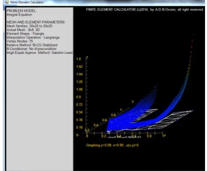
[image:6.595.67.274.406.558.2]Fig. 2 – Profile of Atm. Depression along the Cockpit Example 2: Water Saturation Profile in U shape Reservoir:
Fig. 3 – U Shape Reservoir Layer – Water Saturation Profile, perspective view
V. CONCLUSION
Complex natural phenomena and engineering applications can often be represented by Integral Equations (IE).
Because it could be challenging to solve some of these equations using conventional and/or analytical methods, we use numerical techniques by mean of computers. The most powerful method of the latter is the so called the Finite Element Method (FEM). The FEM refers not only to the partitioning of a domain in smaller pieces called cells or elements, constituting the mesh, but also the use of mathematical polynomials as shape functions, the discretization of the equations, leading to a system of linear equations in matrix format, more suitable for computer iterative solving techniques.
This paper presented our implementation of the FEM using enhanced adaptive meshes to solve and simulate a broad range of real life complex problems that can be formulated in the forms of Integral Equations.
TABLE 2-SYMBOLS
Symbol Description
𝐿𝑝() Functions whose p-th power is Lebesgue integrable ‖𝑓‖𝑋= Norm of 𝑓 in the normed space X
𝑊𝑠,𝑝() Function whose derivatives up to order s are in 𝐿𝑝()
∂𝛼𝑢 ∂
𝑥1 𝛼1… ∂
𝑥𝑑
𝛼𝑑𝑢 is a multi-index ℒ𝑚𝑘(𝑠𝑙) Lagrange Polynomial
𝑔̂𝑖 geometric reference nodes ̂1 geometric reference shape functions
𝛿𝑚𝑙 Kronecker symbol
ACKNOWLEDGEMENT
This paper is submitted as a continuation of my works started during my PhD in Applied Mathematics related to finite element implementation. Therefore, I would like to take this opportunity to express my gratitude to those that have been very supportive and of great help, many of my great colleagues, friends, former teachers, parents and close family, my mother Clementine Avome Ndong and my uncle, Paul Ovono Ndong for their moral encouragements throughout my life and studies.
REFERENCES
[1] Alexandre.Ern, Jean-Luc Guermond, “Theory and Practice of Finite Element”, Springer, Vol.159, 2010
[2] Francis B. Hildebrand, “Methods of Applied Mathematics”, Prentice Hall, The Dover edition, 1992
[3] Dieudonne N. Ovono, PhD Thesis “Implementation of Advanced Finite Element Solution to Complex Problems: Partial Differential, Mixed Problem and Integral Equations”, B.I.U, 2014, p.13-17, p.18-25, p.31-42, p.68-112
[4] C.Antonini, J-F Quint, P.Borgnat, J.Berard, E.Lebeau, E.Souche, A.Chatean, O.Teytaud, “Les Mathématiques pour l’Agrégation (Translation: Mathematics for Aggregation)”, Mai 2002. p.154-161, p.473-499.
[5] R.L. Burden & J.D. Faires, “Numerical Analysis - 9th Edition”,
Brooks/Cole, 2011, Cengage Learning
[image:6.595.63.273.590.763.2]