A Graph-based Decentralization Proposal for
Convex Non Linear Separable Problems with
Linear Constraints
Jaime Cerda, Mario Graff
Abstract—This document proposes several decentralization approaches for the Newton step graph-based model for convex non linear separable problems with linear constraints. The Newton step is well suited for this kind of problems, but when the problem size grows the NLP model will grow in a non linear manner. When this happens, the sparse matrix representation is the path to follow. Furthermore, decentralization schemes are suitable to keep the problem from growing exponentially. In this work a graph based method to achieve this decentralization is proposed. To this end, we have chosen to weak the links, which are part of the graph, as an alternative. These links eventually will guide the solution process in this approach, which implies to weak the links which are coupling the problems in order to achieve such decentralization. A deeper analysis of these links is done which leads to its complete understanding. It will be seen that the main effect of the link weakening operation is to allow the computation of the exact gradient. However, the solution will be reinforced by taking into account the second order information provided by the linking structure. Finally, different decentralisation schemes are presented based on the previous analysis.
Index Terms—Non Linear Separable Programming, Multi-Agent Systems, Decentralised Systems.
NOMENCLATURE N Number of decision variables.
L Number of equality constraints.
M Number of inequality constraints.
zi Decision variable i.
!zi" Upper limit value of variablezi.
#zi$ Lower limit value of variablezi.
zi Slack variable forzi uppper bound.
zi Slack variable forzi lower bound.
∆zi Variablexi increment.
f(z) Objective function gl(z) Equality constraintl.
hm(z) Inequality constraintm.
ali ith coefficient in equality constraint l.
bmi ith coefficient in inequality constraintm.
rl RHS of equality constraint l.
sm RHS of inequality constraintm.
λl Dual variable for equality constraint l.
µm Dual variable for inequality constraintm.
ρi Dual variable forzi uppper bound.
ρi Dual variable forzi lower bound.
℘(S) Power set of set S.
Γi Set of variables connected to zi.
Manuscript received July 23, 2013; revised August 6, 2013. This work was supported by the Scientific Research Coordination, Universidad Michoacana de San Nicolas de Hidalgo
J. Cerda ([email protected]) and M. Graff ([email protected]) are with the Electrical Engineering School, Universidad Michoacana de San Nicolas de Hidalgo, Morelia, Michoacan, Mexico
I. INTRODUCTION
Non linear separable problems (NLSP) are NLPs whose objective function can be decomposed as a sum of functions with only one variable each. The solution of NLSPs are based on very well grounded mathematical theories [1]. This document proposes a Newton step graph-based model to decentralize convex non linear separable problems (NLSP) with linear constraints. Previous works [2], [3], [4], [5] have presented a decentralised approach for NLPs applied to Electrical Power Systems, which rely on the auxiliary principle problem [6]. In this work a graph based method to achieve this decentralization is proposed. To this end, we have chosen to weak the links, which are part of the graph, as an alternative. These links eventually will guide the solution process in this approach, which implies to weak the links which are coupling the problems in order to achieve such decentralization. A deeper analysis of these links is done which leads to its complete understanding. It will be seen that the main effect of the link weakening operation is to allow the computation of the exact gradient. However, the solution will be reinforced by taking into account the second order information provided by the linking structure. This document is structured as follows. First, a graph based model for convex NLSPs with linear constraints is presented. Then, an equivalent graph representation is presented in order to simplify the graph. After this, different decentralisation schemes are presented based on the previous analysis. Finally some conclusions are withdrawn from this proposal.
II. A GRAPH-BASED MODEL FOR CONVEXNLSP
In this section a graph topology for the Newton step method is replicated just as proposed in [7] with the purpose of completeness. To this end, let us base the discussion with the NLSP described by model 1 . This NLSP consists of N variables, L equality constraints, and M inequality constraints.
minz
i
!N
i=1fi(zi)
st. gl(z) = 0, l= 1,2, ..., L (1)
hm(z) ≤ 0, m= 1,2, ..., M
wherefi(zi)are a non linear functions. Furthermore, we
as-sume they have second order derivatives. On the other hand,
gl(z) are linear equalities while hm(z) linear inequalities
L
"
l=1
alizi = rl M
"
m=1
bmizi ≤ sm
In general, a NLP solver starts by building the Lagrangian given by Eq. 2.
L(z) =
N
"
i=1
fi(zi) + L
"
l=1
λlgl(z) + M
"
m=1
µmhm(x) (2)
This is the base to implement the Newton step, whose formulation is given by Eq- 3 [1]:
[image:2.595.129.207.72.138.2]H(L(z))∆z=−∇(L(z)) (3)
Table I, shows the involved elements to compute the Newton step for model 1. Do notice we have introduced slack variables as well dual variables which are used to control the bounds of the decision variables. Here, ρi and zi are used
for the lower bound while ρi andzi are used for the upper
bound ofzi
This model can be represented, as derived in [7], with the graph shown in Fig. 1.
!"#
$
%'"& $!"& %'"#
( & ) & # # # # # # # # # # & & & & # # # !' ( )
-- "1 " " "
1
" " "
) )
)
) )
) )1
# # # # * # # # # # # # # #
-!& &
* * -# & !& # * # )1 ) # # n ) ) ) " " " 1 " # - # ! # #! - # ! ) ) # # * * ! ! & 1 ) # ) # 1 "& &
Fig. 1. Proposed topology for the Newton step method
Each constraint is represented by a dual variable and a set of links which represent the linear terms within the con-straint. The terms in the constraints are represented by links which join the primal variables with the dual variables. The only difference between equality contraints and inequality constraints is the kind of links used to build the linking structure. In the case of equality constraints, the linking structure will be active along the whole solution process. On the other hand, the linking structure for an inequality constraint will be active only when such constraint is binding. This is represented by the gray color given to the links belonging to inequality constraints as opposed to the black links which belong to equality constraints. In table I, the same criterion has been imposed in the elements ofH(L(z)).
As it can be noticed, it is full of empty spaces and gray color, the first are long term sparsity patterns and the second ones are temporary sparsity patterns awaiting to be exploited.
III. ANEQUIVALENTGRAPHREPRESENTATION
In this section, once the characteristics of this graph have been analysed, a simpler graph model representation is derived in order to make its handling easier. This simplifi-cation is based on two main observations: first, the bounding structures are fixed, and second the different kind of variables can be represented in such a way that the content of that node will be inferred by its representation.
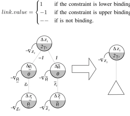
A. An Equivalent Graph Bounding Structure Representation The subgraphs which represent the bound on the variables are well defined. Therefore a special graph notation will be derived in order to handle them, as shown in figure 2. Here all the links and nodes contained in such subgraph are embedded within the triangle. The link value is defined as follows:
link.value=
1 if the constraint is lower binding, −1 if the constraint is upper binding, −− if is not binding.
1 z1
!1 1
z "
−1 1
"z1
! 2#1
1 z " 2 !1 " z 1
!1 !1
! !
"z1
! #1
0 0
"
"
! " ! "
" "
"
z1
z1
z !1 z
!1 1
Fig. 2. Bound subgraph representation
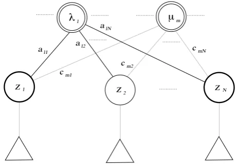
This leads to the representation shown in figure 3.
N
zN
!
!z2
z2
!
! " !!
! ! ! 1 ! ! l2 l1 lN m1 " z ! !z m
!z1
! ! #2 ! #N
0 0
#1
2 2 2
l m l mN m2 a
a a c
c c
Fig. 3. Hessian topology - modified representation
B. An Equivalent Node Type Representation
[image:2.595.308.536.261.463.2] [image:2.595.53.283.394.550.2] [image:2.595.312.540.504.657.2]L(z) =PNi=1fi(zi)−PLl=1λlgl(z)−PmM=1µmhm(z)
∇(L(z)) H(L(z))
zi λl µm ρi ρi zi zi
zi ∇zifi(zi)−λl−µm−ρi+ρi ∇(L(z))2zi ail bim −1 1
λl gl(z) ail
µm hm(z) bim
ρ
i #zi$ −zi+zi 2/2
−1 zi
ρi zi− %zi&+zi2/2 1 zi
zi ρizi zi ρi
zi ρizi zi ρi
TABLE I
THENEWTON STEP INGREDIENTS
nodes in the remaining graph are those representing the primal variables and the dual variables. As mentioned above, the primal variables set can be further divided into two sets. The first one represents those variables which are part of the objective function. The second one contains those primal variables which appear only within the constraints. An instance of these would be the variable representing the electrical angleδin the electric power market example [10],
[11]. These two subsets will be called objective and non-objective variables respectively. Therefore, there are three kinds of variables which have to be represented within the graph e.g. Primal, Dual, Non Objective. These representa-tions are shown in figure 4. Based on the type of variable this node is representing, the information attached to it will be known. This information is as follows
• Objective variables: Attached to this node will be the information in order to be able to compute its gradient if there were no other external information,
• Dual variables: The information attached to this kind of node will be the right hand side of the constraints which will allow its gradient computation.
• Non objective variables: To this node there will be no additional information since its coefficients in the constraints are given by the values of the links which are attached to it, i.e. no second order information is available,
! 0
!
" # g
"
" g
p
! 2$
!
0
"
#
!
g
p "
!
pg
#
"
(b) (a)
(c)
Fig. 4. Variable representation. (a) Primal variable, (b) Dual Variable, (c) Non Objective Variable
This leads to the representation shown in figure 5, where
z2 is assumed as a nonobjective variable. Based on this
graph the appropriate classes for each type of variable can be defined. Once these definitions have been implemented, the operations to solve the graph can be implemented straight-forward.
IV. THEGRAPH ANDITSDECENTRALISATION
In this section the graph and its decentralisation is ad-dressed. To this end an operation over the links of the graph,
zl z
2 zN
m2 l1
m1
l2
m
!
l
!
mN lN
a
a
c
c c
a
Fig. 5. Hessian topology - final equivalent representation
called link weakenning, is defined. This operation is based on the expression derived in [7] as given in eq. 4
∆zi=−∇ziL
(z)
∂2L(z)
∂2zi
− "
∀j∈Γi
(i,j)∈Lk
∂2L(z)
∂zi∂zj
∂2L(z)
∂2zi
∆zj (4)
where Lk denotes the set of links which are taken into
account for this process, do notice|Lk|=k.
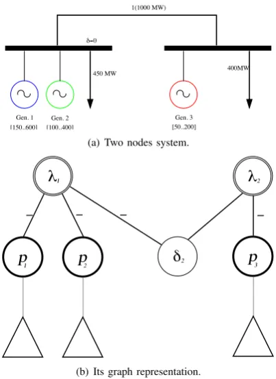
Then, three different approaches to decentralise the graph are proposed. The first one is a complete decentralised, the second approach is based on the notion of the kind of vari-ables within the graph (i.e. primal and dual varivari-ables); and the third approach will be based on agency definitions [9]. To this end let us refer to the system given in [8] as shown in figure 6(a). The graph representation corresponding to this example is shown in figure 6(b), where the minus sign represents a -1 value for the link.
A. Link Weakening
Before going into the decentralisation approaches, let us define the link weakening operation which allows the decentralisaton process. This operation labels the links with one of the following two labels.
• HARD - This labeling will be granted to those links which are not part of the decentralisation process. The graph reduction process will take into account these links,
[image:3.595.139.461.52.166.2] [image:3.595.310.541.202.364.2]!!"
400MW 450 MW
1(1000 MW)
[image:4.595.68.270.50.327.2] [image:4.595.322.526.315.472.2] [image:4.595.66.270.485.646.2]Gen. 2 [100..400] [150..600]
Gen. 1
[50..200] Gen. 3
(a) Two nodes system.
p
1− − − −
1
!
p
2"
p
2
2
!
3
(b) Its graph representation.
Fig. 6. Two nodes system and its graph representation
means to retrieve the actual value of the variable at the other end of the link which will allow the gradient to be computed, as described in [7].
B. A Gradient-oriented Approach
The first approach is to decentralise the graph in an extreme way by weakening all the links as shown in figure 7. This method leads to a model where the gradient method has to be applied at each node in the graph.
1
!
p
2"
p
2
2
!
3
p
1− −
− −
Fig. 7. An gradient-based decentralisation approach
From this figure and based on Eq. 4 we can assert it will become Eq. 5, where the second order information of all of its neighbours is disregarded. In this caseLk=∅. Therefore
Eq. 4 becomes Eq. 5.
∆zi= −∇ziL
(z)
∂2L(z)
∂2zi
(5)
Nevertheless, those nodes which have proper second order information will be able to use it in order to speed up the
convergence process. In particular, all the nodes related to primal variables have this information. Dual variables do not have second order information at all and therefore they will have to use Eq. 6
∆zi=−κ∇ziL(z) (6)
The main drawback of gradient methods known also as steepest descent methods is the hardness to estimate κ. Do
notice that for the primal nodes Eq. 7 holds.
κ= ∂2L1(z)
∂2zi
(7)
C. A Dual-oriented Approach
The second natural approach to decentralise the graph is the dual-oriented approach. From the model proposed in section II it is known the dual variables are in only one layer so if a line across both layers is drawn dissecting the graph, the links which connected the dual variables with the primal variables will be weakened as shown in figure 8.
p
2!
p
2
2
"
3
p
1− −
− −
1
"
Fig. 8. An dual-oriented decentralisation approach
The only dual variables considered in this case are those related with constraints involving two or more primal vari-ables (i.e. bound dual varivari-ables are not split from the primal variables set). Let us denoteDas the set of those dual vari-ables. Therefore Eq. 4 becomes Eq. 8, where all the second order information about the dual variables are disregarded by the primal variables. On the other hand, as the dual variables only have links with primal variables, they are now isolated just as in the gradient approach.
∆zi= −∇ziL
(z)
∂2L(z)
∂2zi
− "
∀j∈Γi
zj∈D/
∂2L(z)
∂zi∂zj
∂2L(z)
∂2zi
∆zj (8)
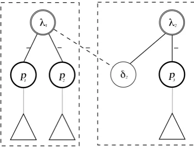
D. An Agent-oriented Approach
In this approach the decentralisation process is made based on concepts drawn from the multiagent community. A classical definition for an agent is
“An agent is a computer systemsituatedin anenvironment, and capable offlexible autonomous actionin thisenvironment in order to meet itsdesign objectives” (adapted from [9]).
independent and proactive behaviour, represented by their ob-jective function. Furthermore, it is situated in an environment which he can sense and act accordingly. However, he is also constrained by its own limitations as well as the constrains presented by the environment. It is important to remark that the agents would be acting on behalf of each node. To cope with this paradigm, the graph is split into subsets of primal variables, links, and dual variables. Based on the membership of these components, the graph is decentralised as shown in figure 9. This approach was the one taken for [10], [11]
2
p
2
2
!
3
p
1− −
1
!
p
"− −
Fig. 9. An agend-based decentralisation approach
V. CONCLUDINGREMARKS
This document has presented a graph-based approach to decentralize a convex NLSP with linear constraints. To this end the main concepts on how to decentralise the graph have been presented. The underlying decentralization principles have been presented based on the analysis of the equation represented by the node and its links. Finally, three decen-tralisation approaches have been described. The first one is a totally decentralised approach which will lead us to a gradient oriented model reinforced with its proper second order information. The second one is based on the type of variables (i.e. primal or dual), and leads us to a horizontal graph split. The last approach is based on concepts drawn from multi-agents community. Finally, even when it has been remarked that this approach is for convex problems, it can be used for non convex problems leading to local optimizers.
REFERENCES
[1] I. Griva, S. G. Nash, and A. Soferr,Linear and nonlinear optimization. SIAM Society for Industrial and Applied Mathematics, 2009. [2] A. G. Bakirtzis and P. N. Biskas, “A decentralized solution of the
dc-opf of interconnected power systems,”IEEE Transactions on Power Systems, vol. 18, no. 3, pp. 1007–1013, August 2003.
[3] A. Bakirtzis, P. N. Biskas, N. Macheras, and N. Pasialis, “A decen-tralized implementation of dc optimal power flow on a network of computers,”IEEE Transactions on Power Systems, vol. 20, no. 1, pp. 25–33, February 2000.
[4] P. Biskas and A. Bakirtzis, “Decentralised opf of large multiarea power systems,”IEE Power, Generation, Transmission and Distribution, vol. 153, no. 1, January 2006.
[5] A. J. Conejo and J. A. Aguado, “Multi-area coordinated decentralized dc optimal power flow,”IEEE Transactions on Power Systems, vol. 13, no. 4, pp. 1272–1278, November 1998.
[6] G. Cohen, “Optimization by decomposition and coordination: A uni-fied approach,”IEEE Transactions on Automatic Control, vol. 2, no. 2, pp. 222–232, 1978.
[7] J. Cerda and J. Avalos, “A graph model proposal for convex non linear separable problems with linear constraints,” in International Conference on Computer Science and Applications 2013. San Francisco, CA, USA: International Association for Engineers, 23-25 October 2013 2013.
[8] J. Cerda and D. De Roure, “A decentralised dc optimal power flow,” in
Proceedings of the Third International Conference on Electric Utility Deregulation and Restructuring and Power Technologies, I. P. E. Society, Ed. Nanjing, China: IEEE Power Engineering Society, April 6–9 2008.
[9] N. Jennings and M. Wooldridge, “Intelligent agents: Theory and practice,” Knowledge Engineering Review, vol. 10, no. 2, pp. 115– 152, 1995.
[10] J. Cerda, D. De Roure, and E. Gerding, “An agent-based electrical power market simulator,” in AAMAS ’08: Proceedings of the 7th International Joint Conference on Autonomous Agents and Multi-agent Systems. Richland, SC: International Foundation for Autonomous Agents and Multiagent Systems, 2008, pp. 1655–1656.
[image:5.595.69.268.187.340.2]