Decision making is an inseparable component of all the activities commonly studied by cognitive psychologists. This is manifested by the prominent role that decision processes play in many areas of cognition, ranging from perceptual processes (Link, 1992) to memory recogni-tion (Ratcliff, 1978) and categorizarecogni-tion (Nosofsky & Pal-meri, 1997). Recently, a convergence of ideas has formed regarding the dynamic nature of the decision process that underlies all the above-mentioned cognitive abilities (cf. Ratcliff, Van Zandt, & McKoon, in press)—namely, the idea that activation for or against each action is sequen-tially sampled, from moment to moment, and accumulated over time. The accumulation process continues until a threshold is reached, at which time a “winner takes all” action is triggered. This sequential sampling type of dy-namic decision process has been highly successful in ex-plaining the effects of time pressure on accuracy and speed –accuracy tradeoff (see Link, 1992; Nosofsky & Pal-meri, 1997; Ratcliff et al., in press).
The broad success of sequential sampling models in perception, memory, and categorization has led some
de-cision researchers to explore their usefulness in the more traditional domain of decision-making tasks, such as risk-taking decisions (Albert, Aschenbrenner, & Schmalhofer, 1989; Aschenbrenner, Albert, & Schmalhofer, 1986; Buse-meyer, 1985; Diederich, 1995; Kornbrot, 1989; Petrusic & Jamieson, 1978; Wallsten, 1995). However, the majority of decision researchers have not followed this lead, and most of the studies in decision making have centered on testing static models originating from economic rather than cognitive theory (see Goldstein & Weber, 1996). Con-sequently, there has been a neglect in conducting inde-pendent tests of the predictions made by sequential sam-pling models of risk-taking decisions. The purpose of this article is to test some basic predictions regarding the ef-fects of time pressure on risk-taking decision making. The risk-taking decision task used for this experiment was developed by Dror, Katona, and Mungur (1998) and is a simplified variant of the game of blackjack. In this task, the decision maker must decide whether or not to gamble by taking another card from a deck in order to max-imize his or her total points without exceeding 21. This task was chosen because the information-processing de-mands (stimulus encoding and response production) are minimal and identical across trials, thus enabling us to iso-late the time pressure effects in the decision stage. Fur-thermore, this task allowed us to systematically manipu-late the levels of risk by varying the probability that taking a card would “bust” (exceed 21).
For this simple task, sequential sampling models make an a priori prediction regarding the effect of time pressure
713 Copyright 1999 Psychonomic Society, Inc.
This research was supported by grants funded by AFRL (awarded to the first author) and by NSF Grant SBR-9602102 and NIMH Grant 5R01MH55680 (awarded to the second author). We thank Zhengping Ma for help with some of the data analyses and Donna Stevens for proofreading the paper. The authors thank the reviewers for very help-ful comments. Correspondence concerning this article should be ad-dressed to I. E. Dror, Department of Psychology, Southampton Univer-sity, Highfield Southampton SO17 1BJ, England (e-mail: dror@cogito. psy.soton.ac.uk). www: http://www.cogsci.soton.ac.uk/~dror
Decision making under time pressure:
An independent test of sequential sampling models
ITIEL E. DROR
Southampton University, Highfield Southampton, England
JEROME R. BUSEMEYER
Indiana University, Bloomington, Indiana
and BETH BASOLA
Southampton University, Highfield Southampton, England
The sequential sampling model also makes specific predictions for this task concerning the mean response times for two different types of responses. A congruent response occurs if a card ischosen when there is very low risk (the response is compatible with the risk level); an incongruent response occurs if a card is not chosen when there is very low risk (the response is not compatible with the risk level). The sequential sampling model predicts that incongruent responses take a longer time to make than congruent responses (see the Appendix for details). A second reason for selecting this task is that a num-ber of studies have investigated the blackjack game, iden-tifying optimal versus heuristic strategies (Anderson & Brown, 1984; Bond, 1974; Keren & Wagenaar, 1985; Phil-lips & Amrhein, 1989). The optimal strategy for maxi-mizing the probability of winning is to take an additional card if the current total falls below an optimal cutoff cri-terion, where this criterion is determined in a complex way that takes into account the card shown for the op-posing player. A common heuristic strategy for this task is the never-bust strategy, which is a conservative tendency to avoid taking an additional card and to stay with the current total. Although nonoptimal, the never-bust strat-egy is attractive because it avoids the possibility of ac-tively taking an action that may be directly responsible for losing the game.
Changes from optimal toward simpler heuristic strate-gies under time pressure provide an alternative explana-tion for the effects of time pressure on risk taking (see, e.g., Johnson, Payne, & Bettman, 1995; Payne, Bettman, & Luce, 1996). However, the predictions inferred from strategy switching differ from the predictions derived from sequential sampling models for this particular task. It is predicted that, in switching to a never-bust strategy under time pressure, the frequency of choosing the gamble never increases (because the likelihood of switching to the sim-pler never-bust strategy increases under time pressure).
Another plausible hypothesis is that participants switch to a fast-guess strategy under time pressure. That is, an individual will occasionally make fast random guesses when under time pressure. Like the sequential sampling model, this fast-guess hypothesis predicts a crossover
in-1993) and comparing the predictions to the actual be-havioral data. In the Discussion section, we review related research on decision making under time pressure and contrast the predictions of sequential sampling models with alternative explanations based on changes in heuris-tic strategies under time pressure.
METHOD Participants
Thirty-two participants (16 males, 16 females) took part in the study for credit in an undergraduate psychology course.
Materials
The decision task was a computer-simulated card game similar to the game of blackjack, where the goal is to maximize the sum of cards without going over 21. The modified blackjack task was de-signed for several purposes. First, it was a simplification of the fa-miliar blackjack game (e.g., in our task, we excluded aces to avoid the ambiguity of whether they should be counted as 1s or 11s and excluded jacks, queens, and kings to avoid issues relating to percep-tual recognition of the face cards; we also did not allow “splitting” and other options that are part of the blackjack game). Second, the probabilities associated with each choice are easily manipulated by the values of the cards dealt to the players, and decisions are easily quantified by the time it takes to make a binary decision (to take an additional card or not).
On each trial, the participant received two cards, which appeared at the top half of the computer screen, and the computer received a single card, which appeared at the bottom half of the screen. Each card was 3.24.9 cm, with its number displayed a single time in the center of the frame, using a 36-size font, Geneva typeface.
The player’s cards were manipulated to vary the level of risk pro-duced by the probability that the player’s total would exceed 21 (and lose the hand). At the very low end of the risk level spectrum were the trials with a sum of 11 or less, in which case there was no risk in taking an additional card (regardless of the value of the additional card, participants could not go over 21). There were also trials with
low risk (trials with sums of 12 or 13), trials with medium risk (tri-als with sums of 14 or 15), tri(tri-als with high risk (trials with sums of 16 or 17), trials with very high risk (trials with sums of 18 or 19), and trials with infinite risk (trials with a sum of 20, in which case it is wrong to take an additional card, because participants would nec-essarily go over 21 and lose their entire hand).
The value showing on the computer’s card was also manipulated on each trial. The computer’s card was programmed to have a low
6, or 7), or a high level (card values of 8, 9, or 10). A high level for the computer card was used to increase the total sum that the player needed to beat the computer and, consequently, increase the play-er’s need to take another card. A low level was used to decrease the total sum that the player needed to beat the computer and, conse-quently, reduce the player’s need to take another card.
Trials were counterbalanced to ensure an equal number of trials with all the possible combinations of player’s and computer’s cards. For each possible sum of the participants’ two cards (17 possible sums, from 4 to 20), a group of 9 trials was constructed, giving a total of 153 trials. Each of the 9 trials in every group was matched to one of the nine possible values of the computer’s card (2–10). The possible combinations of the participants’ cards were also counterbalanced (e.g., for the total sum of 14, all the following combinations were used as equally as possible: 4 and 10, 5 and 9, 6 and 8, 7 and 7, 8 and 6, 9 and 5, and 10 and 4). For administering the task, the 153 trials were organized in a sequence of nine blocks, each consisting of 17 trials. Each block contained a single presentation of all the pos-sible sums of cards, and the order of the trials within the blocks was randomized. (Although this counterbalancing procedure has exper-imental design advantages, it has the disadvantage of influencing the frequencies in such a way that each triple of cards is not equally likely.)
Procedure
The participants were tested individually in a single testing ses-sion. Half the participants were first tested with no time pressure and then with time pressure; the other half of the participants were tested in the reverse order (in each group of participants who were tested in a certain order—either time pressure first or no time pres-sure first—half the participants were male and half were female). For both the time pressure and the no time pressure conditions, the participants were tested on the identical 153 experimental trials, ex-cept that the order of the trials was different (trials were randomized within each block). Time pressure was created by asking the par-ticipants to respond as quickly as possible. It was emphasized that their response time was critical. Under the no time pressure condi-tions, the participants were told to take as much time as they needed to respond and were asked to carefully consider their decisions. The participants were seated approximately 45 cm from the computer screen. Instructions appeared on the computer screen, followed by three practice trials.
At the onset of each trial, an exclamation point was displayed on the computer screen. When the participants were ready to begin the trial, they pressed the space bar. Three cards appeared in each trial; two were considered to be dealt to the participant, and one to the op-ponent. On the basis of the value of these cards, the participant de-cided whether or not to take an additional card (“splitting,” “insur-ance,” and other options from the game of blackjack were not allowed). If a new card was taken, the value of the new card was added to the participant’s total; if the participant decided not to take another card, the total remained unchanged. The participants’ goal was to have the sum of their cards be higher than their opponent’s, without exceeding 21.
The participants were instructed to assume that, after they made their decision, they and their opponent would have the opportunity to take additional cards. They were also informed that they would not see what additional card they received, what additional cards the opponent received, or who won the hand (this was done to en-sure that participants would not change decision strategy or crite-rion during the task as a result of recent positive or negative out-comes of previous decisions; see Dror, Rafaely, & Busemeyer, 1999, and Rafaely, Dror, & Busemeyer, 1998, for details). Rather, after making a decision, the participants would be presented on the next trial with a new and independent sample of cards. If the participants chose to take an additional card, they pressed the yes key (the “b” key, which was labeled yes). If the participants did not want an ad-ditional card, they pressed the no key (the “n” key, which was
la-beled no). After the participants responded, a blank screen appeared for 350 msec, followed by an exclamation point to signal the begin-ning of a new trial. The participants responded yes and no by using two fingers of their dominant hand and pressed the space bar with their nondominant hand. The participants did not receive any feed-back or additional information. Throughout the instructions and practice trials, the participants were encouraged to ask questions, and clarifications were given by the experimenter as needed. How-ever, no talking was allowed during the actual experiment.
RESULTS AND DISCUSSION Empirical Data
First, choice probabilities (proportion of trials in which an additional card was requested) are reported, using the player’s risk level (1no risk, 2low risk, 3medium risk, 4high risk, 5very high risk, 6 infinite risk), the computer’s card level (1low level, 2moderate level, 3high level), and time pressure (no pressure vs. pressure) as within-subjects factors. Second, response times (pooled across choices) are described, using the same three factors. Finally, conditional response times (computed separately for gambling and not gam-bling responses) are shown, using risk category (low risk levels 1, 2, or 3 vs. highrisk levels 4, 5, or 6), time pressure (pressure vs. no pressure), and response cate-gory (choose to gamble vs. choose not to gamble) as fac-tors. (Computer card was omitted because of sample size limitations.)
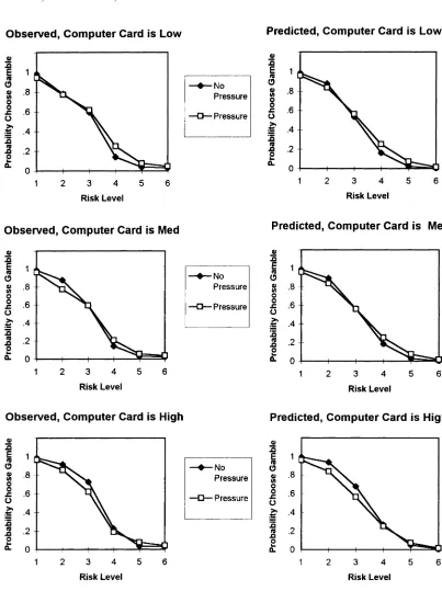
Choice probability. As is illustrated in Figure 1 (left panels), choice probability decreases as risk level in-creases. More important, the curve within each panel for the no time pressure condition is steeper than the corre-sponding curve for the time pressure condition, produc-ing a crossover interaction between risk level and time pressure. This crossover result confirms the a priori pre-diction made by sequential sampling models.
A specific test of the critical risk leveltime pres-sure crossover interaction was performed by computing a single degree of freedom contrast, using the logistic transformed choice proportions as follows. We computed the difference between the no time pressure and time pressure conditions at two different levels of risk, levels 2 and 5. These two levels were chosen because they are moderately extreme, but not to the extent that the choice probabilities approach zero or one. At level 2, the differ-ence was predicted by the sequential sampling models to be positive, and at level 5 it was expected to be negative. We observed the following results: First, the difference between the no pressure and the pressure conditions for the risk level 2 produced a positive contrast equal to +.56; second, the difference between the no pressure and the pressure conditions at risk level 5 produced a nega-tive contrast equal to .32; finally, the contrast of these two differences was significant, according to a ttest [t(155)10.08, p< .0001].
the computer’s card suppressed the tendency to gamble at the low risk levels, whereas a high level for the com-puter’s card enhanced the tendency to gamble at the low risk levels; however, when there was time pressure, the computer’s card had little or no effect on the choice prob-ability. If the data for the time pressure condition is re-plotted with choice probability as a function of risk level and a different curve for each computer card level, the three curves lie virtually right on top of each other. This reflects the fact that the computer card level had no ef-fect under the time pressure condition and suggests that the participants did not have sufficient time and resources to consider the computer’s card.
The trends in Figure 1 are supported by statistical tests obtained from a three-way repeated measures analysis of variance (ANOVA) using the logistic transformed choice proportion for each subject and condition as the depen-dent variable. The main effect of risk level was signifi-cant [F(5,155)178.10, MSe0.514, p< .0001], the risk leveltime pressure interaction was significant [F(5,155)4.68, MSe0.061, p< .0005], and the risk leveltime pressurecomputer card level interaction also was significant [F(10,310)2.32, MSe0.053, p.0121]. The main effect of computer card level was significant [F(2,62)57.31, MSe0.097, p< .0001], the computer card levelrisk level interaction was sig-nificant [F(10,310)15.29, MSe0.076, p< .0001], and the computer card leveltime pressure interaction also was significant [F(2,62)3.29, MSe0.055, p.0440].
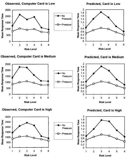
Response time. As is illustrated in Figure 2 (left pan-els), the mean response time is an inverted-U-shaped function of risk level. However, the level of this curve is much lower and the slope is much flatter under the time pressure condition than under the no time pressure con-dition. Finally, the peaks of the curve shift from left to right as the computer card level increases from low to high.
The trends in Figure 2 are supported by statistical tests obtained from a three-way repeated measures ANOVA, using the mean response time for each subject and con-dition as the dependent variable. The main effect of risk level was significant [F(5,155)20.92, MSe1,010,309, p< .0001], the risk leveltime pressure interaction was significant [F(5,155)11.5, MSe642,320, p< .0001], and the risk leveltime pressurecomputer card level interaction also was significant [F(10,310)1.86, MSe 243,049, p.0498]. The main effect of computer card level was significant [F(2,62)3.23, MSe294,584, p.0465], and the computer card levelrisk level interaction was significant [F(10,310)2.90, MSe 274,504, p.0017].
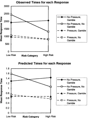
Conditional response time. Figure 3 (top panel) shows the mean response times plotted as a function of risk cat-egory, with a separate line for each response category and time pressure condition. As can be seen in the fig-ure, there is a crossover interaction between risk category and response category, but only for the no time pressure condition. The crossover interaction under the no time pressure condition can be summarized as follows: The
decision to gamble takes less time than the decision not to gamble when the risk category is low, but the decision to gamble takes more time than the decision not to gam-ble when the risk category is high. Recall from Figure 1 that choice probability follows the opposite pattern: The decision to gamble is more frequent than the decision not to gamble under the low risk category, but the decision to gamble is less frequent than the decision not to gamble under the high risk category. This replicates previous find-ings that have shown an inverse relation between the prob-ability that an alternative is chosen and the time required to choose it (Busemeyer, 1982; Petrusic & Jamieson, 1978). The trends in Figure 3 are supported by statistical tests obtained from a three-way repeated measures ANOVA, using the conditional mean response time for each sub-ject and condition as the dependent variable. The risk categorytime pressureresponse category interaction effect was significant [F(1,17)5.557, MSe271,476, p< .05]. (Note: the denominator degrees of freedom re-flect missing observations owing to the fact that some subjects never chose one of the alternatives under some conditions. The analysis with missing cells was com-puted with an SAS system type III sums of squares; see SAS manual, 1996.)
Sequential Sampling Model Predictions
The specific sequential sampling decision model used to generate predictions was derived from decision field theory (Busemeyer & Townsend, 1993; Townsend & Busemeyer, 1996), which is the only sequential sampling model that has been mathematically formalized specifi-cally for risky decision-making tasks. Hence, it enabled us to generate quantitative as well as qualitative predictions for the results of this experiment. Furthermore, decision field theory has been successful in explaining a wide range of fundamental findings from research on risk-taking de-cision making (see Busemeyer & Townsend, 1993).
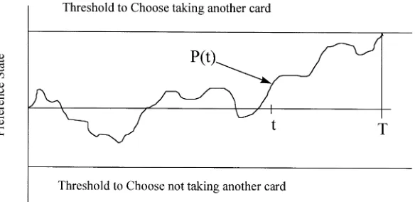
Figure 4 illustrates the basic process that is assumed to occur within a single trial of this decision task. The trial begins at time t0 with the presentation of the play-er’s two cards and the computplay-er’s card; then the player begins the process of deciding whether or not to take an-other card on this trial. The process begins with an ini-tial preference state, denoted P(0), which is equal to zero, assuming that the player starts out unbiased (i.e., P(0) 0). Then, from moment to moment, the player imagines and anticipates the positive or negative outcomes of each choice, given the cards that are presented. At one mo-ment, the player may anticipate winning by taking an ad-ditional card, strengthening the approach tendency, so that P(t1)P(t) > 0. At a later moment, the decision maker may imagine losing the hand by taking an addi-tional card and going over 21, strengthening the avoidance tendency so that P(t2)P(t1) < 0.
becomes strong enough to exceed an inhibitory thresh-old to trigger the action of declining an additional card [P(t) <θ]. The final choice on a particular trial is deter-mined by whether the approach tendency or the avoid-ance tendency crosses the threshold first. The decision time is determined by the time it takes to exceed the threshold magnitude.
According to the model of the decision process de-scribed above, choice and decision time are controlled by two factors: One is θ, the magnitude of the inhibitory threshold; the second is d, the mean change in preference state at each moment. The magnitude of the inhibitory threshold, θ, is assumed to be determined by the time pressure manipulation: The threshold is reduced under the high time pressure condition. The inhibitory thresh-old controls the amount of time spent thinking about the
decision, which in turn controls the amount of informa-tion accumulated about the anticipated outcomes pro-duced by each action. Increasing the threshold increases the average decision time. Thus, more information is ac-cumulated, which causes greater decision accuracy (the probability of choosing the optimal response that maxi-mizes the likelihood of winning). Decreasing the thresh-old (under time pressure) reduces the average decision time. Thus, less information is accumulated, which causes decreased decision accuracy. (See Busemeyer, 1985, for a more formal analysis, or the Appendix.)
The sign of the mean change in preference state, d, de-termines whether the approach or avoidance tendency grows stronger on the average over time. If dis positive, the approach tendency (take another card) grows stronger over time than the avoidance tendency, and if dis nega-Figure 3. The top panel shows the mean response time participants needed for
[image:7.612.164.450.94.476.2]tive, the avoidance tendency (decline another card) grows stronger over time than the approach tendency.
Recall that the probability of exceeding 21 and losing the game by taking another card increases as the player’s total increases, but the need to take another card to beat the computer increases as the value of the computer’s card increases. These two factors are represented in the model by assuming that the mean change in preference state, d, is a decreasing function of the risk level and an increasing function of the computer card level. This im-plies that, for each fixed value of the computer card level, the probability of choosing to gamble will be a decreas-ing function of the risk level (see the Appendix for details). However, under the time pressure condition, there may be insufficient time to consider the computer’s card, so in this case, the computer’s card is ignored. (Changes in at-tention over time are consistent with Diederich’s [1995] multiattribute generalization of decision field theory.)
The mathematics used to derive the formulas for this particular model have been presented elsewhere (Buse-meyer & Townsend, 1992, 1993), and the Appendix pro-vides the derived formulas used to compute the predic-tions shown below. It is important to note that strong quantitative tests of the model are made possible through the use of both choice probability and choice response time measures of preference. The basic method for test-ing the model is first to estimate the model parameters from the choice probability data and then to use these same parameters to generate parameter-free predictions for the mean response time data.
More specifically, seven model parameters were esti-mated from the 36 observed choice proportions, and these parameter estimates were used in the formulas to com-pute the choice probabilities from the model. The criti-cal test is obtained by entering these same seven param-eters into the formulas for computing the predictions for choice response time data. This provides a generaliza-tion test of the model by producing predicgeneraliza-tions for all of the response time data that do not require estimating any new parameters.
First, the right-hand panels of Figure 1 illustrate the fits to the choice probability data. As can be seen by com-paring the left and the right panels, the model correctly reproduces the crossover interaction between risk level and time pressure, and it also reproduces the effects of computer card level on choice probability. Although the specific form of the curves producing the crossover inter-action depends on the estimated parameters, the backward-S-shaped form of the function, as well as the crossover interaction, is a necessary property of the model. In par-ticular, if the data failed to show this crossover, the model would be unable to fit the results.1
[image:8.612.162.454.92.234.2]Second, the right-hand panels of Figure 2 illustrate the predictions for the response time data. Note that these predictions are made without using any parameters (this includes the time unit for the predictions, so only the pat-tern of the predictions is important). As can be seen by comparing the left and the right panels, the model cor-rectly predicts the inverted-U-shaped function relating re-sponse time and risk level, and the model also correctly Figure 4. A model of the task based on decision field theory. The horizontal axis
predicts the proportional reduction in response time at each risk level produced by the time pressure manipula-tion. Finally, the model correctly predicts the shift in the peak of this U-shaped function with increases in the computer card level.
A strong test of the model is obtained by evaluating the predictions for decision times conditioned on the specific choice (the response chosen). The model cor-rectly predicts that the mean time to take another card is shorter than the mean time to choose to not take another
card, when the risk level is relatively low. The model also correctly predicts the opposite order when the risk level is relatively high. Furthermore, the model predicts that this crossover interaction effect is attenuated by time pressure (see the bottom part in Figure 3).
Strategy-Switching Model Predictions
An alternative explanation for the effects of time pres-sure on decision behavior is that subjects switch to sim-pler heuristic strategies under time pressure. Two
[image:9.612.168.453.202.673.2]model by fitting it to the choice data and mean response time data with one major change (see the Appendix for details). Instead of decreasing the threshold bound under time pressure conditions, this parameter was held con-stant, and a new parameter was added, representing the probability of fast guessing under time pressure. In sum, seven parameters (six original plus one fast guess) were estimated from the choice probability data, and these same parameters were used to make predictions regard-ing decision time. This model produced essentially the same fit to the choice probability data as the original se-quential sampling model.
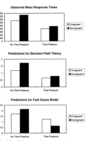
The critical test of the sequential sampling model ver-sus the fast-guess model is shown in Figure 5. The top panel shows the observed mean time to make congruent (white bar) versus incongruent (dark bar) choices, where a congruent choice was to take another card under very low risk (levels 1 or 2) and an incongruent choice was the decision not to take a card under these same condi-tions.2The left pair of bars represents the no time pressure condition, and the right pair represents the time pressure condition. Note that the incongruent responses were made more slowly than the congruent responses under the crit-ical time pressure condition.3
The middle panel shows the corresponding predictions of the original sequential sampling model. As can be seen in the figure, the original sequential sampling model accurately predicts the pattern of observed results under both time pressure conditions. The bottom panel shows the corresponding predictions produced by the fast-guess model. As can be seen, the fast-guess model fails to de-scribe the pattern of results under the time pressure condi-tion. In sum, the finding of slower incongruent responses, as compared with congruent responses, is contrary to the fast-guess model and supports the original sequential sampling model.
GENERAL DISCUSSION
Recent emphasis has been placed on the decision pro-cess in numerous sucpro-cessful models from a variety of cognitive domains (Link, 1992; Nosofsky & Palmeri, 1997; Ratcliff, 1978; Smith, 1995). It seemed interest-ing to examine this decision process in the more “pure”
mathematically developed for risky decision making and, thus, it enabled us to make precise predictions for our behavioral gambling-like task.
Our behavioral data were consistent with previous be-havioral research (Dror et al., 1998), showing that par-ticipants systematically were less likely to take a card as the risks increased and that response time for making the decisions decreased as the risks were toward the ends of the risk level spectrum. Our manipulation of time pres-sure caused a polarization effect; participants were more conservative and less likely to take an action (request an additional card) at the lower levels of risk and were more risky and likely to take an action at the higher levels of risk. That is, the S-shaped choice probability curve, as a function of risk, was flatter under the time pressure con-dition. Response times decreased with time pressure, and the inverted-U-shaped choice time curve, as a func-tion of risk, was also flatter under the time pressure con-dition. Finally, the time to make a choice was inversely related to the probability of making that choice, repli-cating previous findings (Busemeyer, 1982; Petrusic & Jamieson, 1978).
(1985) have identified two such strategies in blackjack-type tasks (see, also, Anderson & Brown, 1984; Bond, 1974; Phillips & Amrhein, 1989). First, the basic strat-egy, which is the optimal strategy that maximizes the probability of winning, requires the player to consider his or her own cards as well as the computer’s card. Sec-ond, the never-bust strategy is a conservative tendency to avoid taking an additional card and to stay with the cur-rent total. Note that the never-bust strategy only requires attention to the player’s cards and does not require atten-tion to the computer’s card. Although nonoptimal, the never-bust strategy is attractive because it is simple and, more important, avoids the possibility of actively taking an action (requesting an additional card) that may be di-rectly responsible for losing the game.
The basic or optimal strategy for our risk-taking task is to always choose to take an additional card if the cur-rent total sum of the cards falls below a cutoff criterion (this criterion depends on, among other things, the com-puter’s card). In other words, if we were to plot the choice probability curve predicted by this strategy (similar to that shown in Figure 1), it would be a backward step function with an abrupt jump from one to zero at the cutoff. How-ever, if this cutoff varies across participants, the curve pro-duced by averaging across participants would appear as a backward-S-shaped curve like that shown in Figure 1. The never-bust strategy is a very simple heuristic strat-egy of not taking an additional card if there is some risk that the player’s new total will exceed 21. It is reasonable to expect that, under time pressure, at least on some pro-portion of trials, participants may abandon the more dif-ficult process of locating the optimal cutoff for the sim-pler heuristic strategy that guarantees not losing the entire hand by taking an additional card. However, this strategy-switching model does make one important distinguish-ing prediction. That is, the curve produced under time pressure must lay completely below that predicted by no time pressure (because the proportion of trials in which participants use the simpler strategy of not taking an ad-ditional card always increases under time pressure). How-ever, as is apparent in Figure 1 (top panel), our data do not support this prediction.
Another plausible heuristic strategy is to resort to fast random guesses under time pressure. This fast-guess model explains the time pressurerisk level crossover interaction effect on choice probability as being the re-sult of mixing random guesses on some proportion of tri-als, which flattens out the backward-S-shaped curve. However, the fast-guess model incorrectly predicts that subjects will make faster incongruent, as opposed to congruent, responses under time pressure, which is con-trary to the observed results.
In sum, for this particular task, the never-bust and fast-guess strategies are the most common and obvious heuris-tics, and we can rule out the hypothesis that participants tend to switch to these particular strategies under time
pressure. In contrast, the sequential sampling model pro-vides a comprehensive explanation of both the choice probability and the choice response time behavioral data. Of course, it is impossible to enumerate all conceivable strategies, so we cannot completely eliminate the general form of this explanation. Moreover, one could interpret changes in attention to the opponent’s card as a kind of strategy switch. But then the notion of strategy becomes so broad that one has to question its testability or pre-dictive utility.
One final comment is that our results do not rule out other possible effects of time pressure on decision pro-cesses, such as a speed-up of each processing step (see Ben Zur & Breznitz, 1981). But note that simply speed-ing up processspeed-ing by a constant factor under time pressure cannot explain the changes in the pattern of choice prob-abilities and response times produced by time pressure.
It is interesting to note that our empirical results, ob-tained from a traditional decision-making task, appear to be very similar to the speed –accuracy tradeoff results found in other cognitive tasks, such as perception (see Link, 1992), memory (see Ratcliff, 1978), and catego-rization (see Nosofsky & Palmeri, 1997). Furthermore, the success of sequential sampling models in accounting for the results obtained from this risk-taking decision-making task strengthens our confidence in the general use of this decision process across a variety of cognitive tasks (for further discussion on the usefulness of such models, see Dror & Gallogly, 1999). In summary, both the em-pirical results and the theoretical analyses presented in this study support the view that common principles of de-cision processes underlie a wide range of cognitive tasks.
REFERENCES
Albert, D., Aschenbrenner, K. M., & Schmalhofer, F.(1989). Cognitive choice processes and the attitude–behavior relation. In A. Upmeyer (Ed.), Attitudes and behavioral decisions (pp. 61-99). New York: Springer-Verlag.
Anderson, G., & Brown, R. I.(1984). Real and laboratory gambling, sensation-seeking and arousal. British Journal of Psychology, 75, 401-410.
Aschenbrenner, K. M., Albert, D., & Schmalhofer, F.(1986). Sto-chastic choice heuristics. Acta Psychologica, 56, 153-166. Ben Zur, H., & Breznitz, S. J.(1981). The effect of time pressure on
risky choice behavior. Acta Psychologica, 47, 89-104.
Bond, N. (1974). Basic strategy and expectation in casino blackjack.
Organizational Behavior & Human Performance, 12, 413-428. Busemeyer, J. R. (1982). Choice behavior in a sequential decision making
task. Organizational Behavior & Human Performance, 29, 175-207. Busemeyer, J. R. (1985). Decision making under uncertainty: A com-parison of simple scalability, fixed sample, and sequential sampling models. Journal of Experimental Psychology: Learning, Memory, & Cognition, 11, 538-564.
Busemeyer, J. R., & Townsend, J. T. (1992). Fundamental derivations for decision field theory. Mathematical Social Sciences, 23, 255-282. Busemeyer, J. R., & Townsend, J. T. (1993). Decision field theory: A dynamic-cognitive approach to decision making in an uncertain en-vironment. Psychological Review, 100, 432-459.
Junger-time constraints. In O. Svenson & J. Maule (Eds.), Time pressure and stress in human judgment and decision making (pp. 167-178). New York: Plenum.
Keren, G. B., & Wagenaar, W. A. (1985). On the psychology of play-ing blackjack: Normative and descriptive considerations with impli-cations for decision theory. Journal of Experimental Psychology: General, 114, 113-158.
Kornbrot, D. E.(1989). Random walk models of binary choice: The effect of deadlines in the presence of asymmetric payoffs. Acta Psy-chologica, 72, 103.
Link, S. W.(1992). The wave theory of difference similarity. Hillsdale, NJ: Erlbaum.
Nosofsky, R. M., & Palmeri, T. J. (1997). An exemplar based random walk model of speeded classification. Psychological Review, 104, 266-300.
Payne, J. W., Bettman, J. R., & Luce, M. F. (1996). When time is money: Decision behavior under opportunity– cost time pressure. Or-ganizational Behavior & Human Decision Processes, 66, 131-152. Petrusic, W. M., & Jamieson, D. G. (1978). Relation between
proba-bility of preferential choice and time to choose changes with practice.
Journal of Experimental Psychology: Human Perception & Perfor-mance, 4, 471-482.
Phillips, J. G., & Amrhein, P. C. (1989). Factors influencing wagers in simulated blackjack. Journal of Gambling Behavior, 5, 99-111. Rafaely, V., Dror, I. E., & Busemeyer, J. R. (1998). The
susceptibil-ity of young and old adults to positive and negative outcomes of re-cent decisions. Abstracts of the Psychonomic Society, 3, 41. Ratcliff, R. (1978). A theory of memory retrieval. Psychological
Re-view, 85, 59-108.
Ratcliff, R., Van Zandt, T., & McKoon, G.(in press). Connectionist and diffusion models of reaction time. Psychological Review. Smith, P. L. (1995). Psychophysically principled models of visual
sim-ple reaction time. Psychological Review, 102, 567-593.
Svenson, O., & Maule, J.(1995). Time pressure and stress in human judgment and decision making. New York: Plenum.
Townsend, J. T., & Busemeyer, J. R. (1996). Dynamic representation of decision-making. In R. F. Port & T. van Gelder (Eds.), Mind as mo-tion: Explorations in the dynamics of cognition. Cambridge, MA: MIT Press.
Wallsten, T. S. (1995). Time pressure and payoff effects on multi-dimensional probabilistic inference. In O. Svenson & J. Maule (Eds.),
Time pressure and stress in human judgment and decision making
(pp. 167-178). New York: Plenum.
NOTES
1. Note that the above model assumes that time pressure has two sep-arate effects on the decision process. One is a decrease in the threshold bound, and the second is a decrease in attention to the opponent’s card. One might question whether both of these assumptions are really nec-essary. To answer this question, the model was refit under two different constraints. On the one hand, when the model was refit assuming a de-crease in threshold but no dede-crease in attention under time pressure, the
2. Risk level 3 was included in Figure 3 in order to include all of the data in the basic analyses. Risk level 3 was not included in Figure 5 because this risk level was too high to treat choosing no card as an incongruent response. In other words, risk level 3 does entail some risk, which makes it an ambiguous case for defining the choice of no card as an incongru-ent response.
3. A dependent ttest was used to perform a statistical test of the hy-pothesis implied by the fast-guess model. Define µCand µIas the pop-ulation mean response times for the congruent and incongruent re-sponses, respectively, under time pressure. To falsify the fast-guess model, we need to reject the directional hypothesis H0: (µIµC) < 0. The
sample mean difference between congruent and incongruent response times under time pressure produced a tstatistic that exceeded the con-ventional cutoff for rejecting this hypothesis [t(31)1.8, p< .05].
APPENDIX
The purpose of this appendix is to present the formulas used to compute the predictions from the model derived from deci-sion field theory for this task. Decideci-sion field theory has seven stages, but it was sufficient to use only stage three (Equations 3c and 3d in Busemeyer & Townsend, 1993) for this simple task. In this case, the formula for the probability of choosing to gamble for an individual, denoted Pr[G], derived from the gen-eral theory for this task, is
Pr[G]1/[1exp(2θd)]. (1)
Note that this is an S-shaped logistic function of the mean change in preference state, d, and that the threshold, θ, moderates the slope of this logistic function. Recall that dis inversely related to the risk level, and therefore, choice probability is predicted to be a backward-S-shaped function of risk level. Increasing the time pressure decreases θ, which decreases the slope of the lo-gistic function of d, and this produces the predicted crossover interaction.
The mean time to make a choice for an individual subject, denoted E[T], derived from the general theory for this task, is
E[T](θ/d) (2Pr[G]1). (2)
Conceptually, the ratio (θ/d) can be interpreted as the well-known formula, travel time equals distance divided by rate of travel. Under time pressure, the distance to travel θdecreases, so that the time to travel also decreases. Note that this equation does not include a time unit for the decision process, and so the time constants for the predicted and observed times are not equated. Thus, the predicted times are only proportional to the observed times.
min-imized the sum of squared deviations between the predicted and the observed choice probabilities. Two of the seven parameters were used to estimate two threshold values (θ1.44 for the no time pressure condition, and θ0.955 for the time pressure condition).
Four parameters were used to determine the mean change in preference, d, for each of the 36 conditions, as follows. Denote
di jkas the mean change in preference under risk level i(i1, 2, 3, 4, 5, 6), computer card level j (j1, 2, 3), and time pres-sure condition k(k0,1). The following expression was used to determine the mean change:
dijk[(1 k) cja(i3.5)]. (3)
When k0 (no time pressure), the mean change equals the dif-ference between the effect of the computer card level and the ef-fect of the risk level; when k1 (time pressure present), the ef-fect of the computer card is eliminated, and the mean change is inversely related to the effect of the risk level. The effect of risk level was assumed to be proportional to the risk level, with the constant of proportionality estimated from the choice data (a
.842). Three parameters were estimated from the choice data to represent the effect of the computer card level (c12.85, c2
2.92, c33.14).
An additional seventh parameter was used to incorporate in-dividual differences into the model. This was accomplished by adding a random effect Slto Equation 3:
dijkl[(1k) cja(i3.5Sl)]. (4)
Conceptually, negative values of Slrepresent individuals that are more risk seeking than the average person and positive val-ues of Slrepresent individuals who are more risk aversive than the average person. In general, the distribution of individual difference effects is unknown. For simplicity, the individual dif-ference effects Slwere represented by a binomial distribution across the values {1.5,1.0,0.5, 0, 0.5, 1.0, 1.5} with a parameter p.42 (estimated from the choice data). Specifi-cally, the probability of Slwas computed by
P[Sls][(6!)/(2s 3)!(3 2s)!] p2s 3(1 p)3 2s. (5)
To summarize, the choice probabilities and mean response times were computed separately for each condition and each value of the individual difference effect Sl, using Equations 1, 2, and 4, and then these predicted values were averaged across the individual differences Slfor each condition, using the prob-abilities defined by Equation 5. The seven parameters were es-timated with the choice probability data alone, and then these same seven parameters were used to compute the mean re-sponse times shown in Figure 3 and Figure 5.
The fast-guess model is obtained by employing Equations 1 and 2 directly for the no time pressure conditions and by modify-ing Equations 1 and 2 by mixmodify-ing a guessmodify-ing probability, g, under time pressure:
Pr[G](1g) /[1exp(2θd)](.5)g, (6)
and
E[T] (1g) (θ/d) (2Pr[G]1)gTg, (7)
where Tgis the mean time required to make a fast guess. The mean time to make a fast guess cannot be estimated from the choice data alone. Therefore, it was necessary to estimate eight pa-rameters from both the choice and the mean response time data: a threshold, θ, constant across time pressure conditions; a guess-ing rate gunder time pressure; three coefficients for the com-puter card; two coefficients, aand p, described earlier, used to determine the mean change for each condition and individual; and, finally, the mean time to make a guess, Tg. These eight pa-rameters were then used to compute the mean times to make congruent and incongruent responses, shown in Figure 5.
As Figure 5 shows, the predictions computed from the deci-sion field model indicate that the mean response time under very low risk is slower for incongruent responses than for gruent responses for both time pressure conditions. The con-ceptual reason for this prediction is that, when the risk level is very low, incongruent responses tend to be chosen when the mean change in preference for an individual (Equation 4) is small in magnitude; when this occurs, the rate of travel (see Equation 2) slows down the time reach the boundary for both time pressure conditions. For example, when the risk level is very low but an individual is very risk aversive, the mean change in preference will be close to zero; this is the case that is most likely to pro-duce an incongruent response, but this response also tends to take more time because of the slow rate of travel.
In contrast, the predictions computed from the fast-guess model indicate that incongruent responses are faster than con-gruent responses under time pressure and very low risk. The conceptual reason for this prediction is that the fast-guess model assumes that a change in decision strategy occurs under time pressure. Thus, it predicts the same result as the decision field model with no time pressure. But under time pressure, the in-congruent responses tend to be produced by the fast guesses, which makes the incongruent responses faster than the congru-ent responses (the latter tend to occur after waiting to reach the criterion bound).