AdS/CFT Correspondence
Lorenzo Gerotto
School of Mathematics, Trinity College Dublin
College Green, Dublin 2, Ireland
A thesis submitted to the University of Dublin in fulfillment of the requirements for the degree of
Doctor in Philosophy
Supervisor:Dr. Tristan McLoughlin
Declaration
I declare that this thesis has not been submitted as an exercise for a degree at this or any other university and it is entirely my own work.
I agree to deposit this thesis in the University’s open access institutional repository or allow the Library to do so on my behalf, subject to Irish Copyright Legislation and Trinity College Library conditions of use and acknowledgement.
This thesis is based in part on the articles [1].
Signed:
Summary
Form factors are matrix elements of local operators between scattering states, and are interesting off-shell objects in any QFT. The main objective of this thesis is to compute form factors perturbatively in the world-sheet theory describing strings in AdS5×S5, in the Landau–Lifshitz model and in a number of its generalizations.
The S-matrix bootstrap allows to determine completely the scattering processes of an integrable two-dimensional QFT. The world-sheet theory for type IIB superstrings in AdS5×S5is believed to be integrable and the S-matrix has been computed, though we do not have a complete bootstrap program for the form factors yet. This would amount to solving the relevant set of form factor axioms. These are consistency con-ditions which, for a massive integrable relativistic theory, can be derived from the validity of the LSZ formalism and the hypothesis of “maximal analyticity”, and allow in principle to write any form factor explicitly from the knowledge of the S-matrix. Analogous axioms for the world-sheet have been proposed, however finding a gen-eral solution for said axioms is still an open problem.
Perturbative form factor calculations have been already carried out for thesu(2)
sector of the world-sheet string. One of the goals of this thesis is to extend this com-putation of the tree-level three-particle form factor to the full theory. We also discuss a particular configuration, the so-called diagonal form factors, which are related to the structure constants of “Heavy-Heavy-Light" three-point functions in the string field theory.
We also study the Landau–Lifshitz model, a non-relativistic theory that can be obtained as a thermodynamic limit of the Heisenberg XXX1/2 spin chain, which is related to the dilatation operator in N = 4 SYM. The LL model also emerges as a double limit of the AdS5×S5string, and it has proved a useful tool in the context of the AdS/CFT correspondence to better understand the matching between the energies of on-shell string states and the anomalous dimensions of SYM operators. To study the higher-order contributions, we will work with a generalized LL model which includes all the terms allowed by symmetry at that order with generic constants. These can be fixed to match the “gauge”- or “string”-LL model, since it has been proved that the two models match only up toO(λ2).
Acknowledgements
I wish to thank first and foremost my supervisor Tristan McLoughlin for his guid-ance. He has always been happy to help, gently pushing my work in the right di-rection and patiently clarifying any doubt I had. Needless to say that without his support and understanding this thesis would not exist.
I am grateful to everyone in the School of Mathematics at Trinity College Dublin for creating a pleasurable and stimulating environment, including many entertaining lunches and many interesting seminars. In particular I wish to thank Sergei Frolov, Manuela Kulaxizi, Jan Manschot, Tristan McLoughlin, Andrei Parnachev, Samson Shatashvili, Stefan Sint, and Dmytro Volin.
I also thank my fellow Ph.D. students Argia, Christian, David, Georgios, Kiko, Martijn, Philipp, not only for the useful weekly discussions. A special thank-you goes to Philipp and Christian for sharing the office and the whole experience.
Thanks to all the people I have met during conferences and seminars, especially the organizers and participants of the Young Researcher School of Integrability in Durham and the follow-up in Dublin.
Contents
Declaration iii
Summary v
Acknowledgements vii
1 Introduction 1
1.1 The AdS/CFT correspondence . . . 1
1.2 Integrability in AdS/CFT . . . 2
1.3 Form Factors . . . 3
1.4 The Landau–Lifshitz model . . . 4
1.5 Plan of the thesis . . . 6
2 Superstring theory on AdS5×S5 7 2.1 The AdS5×S5superstring . . . 7
2.1.1 The bosonic string . . . 7
2.1.2 The uniform light-cone gauge . . . 9
2.1.3 The action for the AdS5×S5string . . . 12
The coset action . . . 13
Light-cone gauge . . . 14
Decompactification limit . . . 14
The large tension expansion . . . 15
Thepsuc(2|2)algebra . . . 17
The world-sheet action . . . 18
2.1.4 Quantization in light-cone gauge . . . 19
2.1.5 The world-sheet S-matrix . . . 22
2.2 World-sheet symmetries . . . 23
2.2.2 Charges and currents . . . 24
2.2.3 Hopf Algebra interpretation . . . 26
2.2.4 Adjoint actions . . . 33
2.2.5 A linear basis and a dual algebra . . . 35
2.2.6 Asymptotic symmetries . . . 44
3 Integrability in the AdS/CFT correspondence 47 3.1 N =4 supersymmetric Yang–Mills theory . . . 47
3.1.1 TheN =4 SYM action . . . 47
3.1.2 N =4 SYM symmetries . . . 48
3.1.3 Primary operators and scaling dimensions . . . 50
3.1.4 Correlation functions . . . 51
3.1.5 Spin chains andN =4 SYM . . . 53
3.2 The Bethe ansatz for the XXX1/2spin chain . . . 55
3.2.1 The Heisenberg XXX spin chain . . . 55
3.2.2 The coordinate Bethe ansatz . . . 57
3.2.3 The algebraic Bethe ansatz . . . 60
4 Form Factors 63 4.1 Definitions . . . 63
4.1.1 Generalized form factors . . . 63
4.1.2 Diagonal form factors . . . 65
Finite volume . . . 67
4.1.3 Form factor axioms . . . 68
4.2 Perturbative calculations . . . 71
4.2.1 Perturbative world-sheet form factors . . . 71
World-sheet propagators . . . 72
One-particle form factors . . . 73
Three-particle ff: bosonic operators . . . 74
Three-particle ff: fermionic operators . . . 76
4.2.2 The form factors in the near-flat limit . . . 77
5 The Landau–Lifshitz model 85
5.1 The Landau–Lifshitz model and the AdS/CFT correspondence . . . . 85
5.1.1 The LL action . . . 85
5.1.2 Spin chains and the LL model . . . 86
5.1.3 The LL model as a limit of the light-cone string action . . . 88
5.1.4 The SU(3) LL model . . . 90
5.2 The generalized LL model . . . 93
5.2.1 Perturbative Quantization . . . 93
5.2.2 The action of the generalized LL model . . . 95
5.2.3 Feynman rules . . . 97
5.2.4 The Landau-Lifshitz S-matrix . . . 98
5.3 Diagonal form factors in the Landau–Lifshitz model . . . 101
5.3.1 |ϕ|2-Operator . . . 101
5.3.2 |ϕ|4-Operator . . . 107
5.3.3 The spin-chain S-matrix and its LL limit . . . 109
5.3.4 Form Factors from the XXX spin-chain . . . 112
5.4 Form Factor Perturbation Theory . . . 118
5.4.1 Marginal Deformations . . . 120
5.4.2 Deformed Landau-Lifshitz . . . 121
5.4.3 Deformed LL from Form Factor Perturbations . . . 123
Conclusions 129 A Introduction to the S-matrix 131 A.1 The definition . . . 131
A.2 S-matrix bootstrap . . . 134
B Global Symmetry Currents 135
C Asymptotic Fields 139
D Hopf Algebra Consistency Conditions 141
E AdS strings/gauge theory duality 143
Chapter 1
Introduction
1.1
The AdS/CFT correspondence
The idea of a correspondence between a gauge theory of particle interactions and a theory describing vibrating strings has its roots in the attempt to give an adequate description of strongly correlated quantum field theories (QFT), such as quantum chromodynamics (QCD), which describes quarks and gluons. In particular, the goal was to gain novel insights into the strong regime of QCD through the study of a dual theory at weak coupling.
After much progress on the string theory side, the turning point was Maldacena’s seminal paper [2] in 1997, where he proposed a relationship (duality) between su-perstrings on anti-de Sitter (AdS) backgrounds and (super)conformal field theories (CFT), which is now known as the AdS/CFT correspondence or more generally as gauge/gravity duality. In particular, he noticed that the type IIB string on the ten-di-mensional curved background AdS5×S5was related toN =4 supersymmetric Yang– Mills theory (SYM) with gauge groupSU(N). The assumption is that the two theories are equivalent in the sense that we can build a precise dictionary between the objects on the string side and those on the gauge side, and computations of corresponding physical quantities yield identical results. The starting point for the comparison is the following conjectured relation between the parameters of the two theories
R4
α02 = g 2
YMN, 4πgs= g2YM, (1.1.1)
where gYM is the SYM coupling constant, N the degree of the gauge group, gs the
andS5spaces.
A key characteristic of the gauge/string duality is that it relates strongly coupled sectors on one side to weakly coupled sectors in the corresponding theory. Thus it provides a method to study perturbatively the strongly interacting regime of gauge theories, and it also allows to explore quantum gravity through gauge theory com-putations. On the other hand, the strong-weak relations make testing the AdS/CFT correspondence a challenging task. Crucial steps in this direction were made in 2002 by Berenstein, Maldacena and Nastase [3] and by Minahan and Zarembo [4].
At first the analysis was focused on the low-energy limit of specific string so-lutions and protected SYM operators, i.e. those not receiving quantum corrections, the goal being to compare the energy of the strings with the conformal dimensions of the operators (the eigenvalues of the dilatation operator). The idea of BMN was to consider instead a particular limit1 of the AdS
5×S5 string, which corresponds to unprotected operators with large R-charge. Minahan and Zarembo noticed that the terms in theλ-expansion of the dilatation operatorDare equal to the Hamiltonian of some integrable spin chain [4], which is a one-dimensional lattice model with a spin representation in every site. This means that we can find the loop corrections to the classical dimension by solving the corresponding spin chain. The computations are greatly simplified since we can utilize the useful tools of integrability built over the years, starting from Bethe’s 1931 ansatz method [5] to solve the spectral problem, i.e. to find eigenvalues and eigenvectors of the spin-chain Hamiltonian.
1.2
Integrability in AdS/CFT
The integrable structure inN =4 super Yang–Mills, and in the corresponding string theory, is of the type usually associated with two-dimensional systems, such as the Heisenberg XXX1/2ferromagnet. This is the first example of a non-trivial four-dimen-sional integrable theory, and it has led to a great improvement in our understanding of both string theory and SYM, see [6] for a detailed review. In principle, integrability allows to obtain any quantity of the theory exactly (non perturbatively), though in
1BMN studied strings on the plane-wave background, which can be obtained as a Penrose limit of
AdS5×S5. However, in order to obtain the complete algebraic structure (two centrally extendedsu(2|2))
practice we expect to be able to write down the equations but not always to be able to solve them.
To see how integrability emerges in the AdS/CFT correspondence, we need to re-call that in conformal theories, the structure of the two-point functions is completely determined by their conformal dimensions, i.e. the eigenvalues of the dilatation op-eratorD. For small values of the ’t Hooft couplingλ= g2YMN, theN =4 super-Yang-Mills (SYM) dilatation generator can be computed perturbatively as
D= ∞
∑
r=0
λ 16π2
r
D2r. (1.2.1)
If we restrict ourselves for simplicity to single trace operators composed of just two types of complex scalars, that is an su(2)sub-sector of the full theory, the one-loop part can be mapped to the Heisenberg XXX1/2spin-chain Hamiltonian [4]
H=2
L
∑
`=1(1−P`,`+1), (1.2.2)
whereP`,`+1is the permutation operator acting on sites`and`+1. The eigenvalues and eigenvectors of the spin-chain Hamiltonian (1.2.2) can be found by using integra-bility techniques such as the coordinate Bethe ansatz [5] or the algebraic Bethe ansatz (reviewed in [7]), where we can write explicitly the conserved charges to show the in-tegrability of the model. Higher orders inλin the expansion of the dilatation operator (1.2.1) correspond to Hamiltonian of spin-chains with longer range interactions.
1.3
Form Factors
the theory, with the assumptions of unitarity and analyticity, thanks to the bootstrap program [8], see also [9].
The S-matrix can also be used to calculate off-shell quantities, such as the form factors, which are matrix elements of local operators between scattering states. Ex-plicitly we can define the form factor of the operator at the originO(~x =0)in terms of the particles’ momentapi as
FO;i0m,...,i01
i1,...,in (p 0
m, . . . ,p01|p1, . . . ,pn) =i
0
m,...,i01p0
m, . . . ,p10
O(0)|p1, . . . ,pnii
1,...,in . (1.3.1)
According to the bootstrap approach, in principle we should be able to derive the form factors for an integrable two-dimensional QFT from the knowledge of the S-matrix and the symmetries of the theory, solving the so-called form factor axioms [10]. The axioms are a set of consistency conditions, which have been written for a relativistic theory in [11] and for the world-sheet string in [12, 13], though their general solutions are not known.
The diagonal form factors are a special class of form factors in which the two asymptotic states are taken to be identical, i.e. n = mand|p01, . . . ,p0mi= |p1, . . . ,pni
in (1.3.1). These are particularly interesting in the context of the AdS/CFT correspon-dence as they are related to the structure constants of “Heavy-Heavy-Light" three-point functions [14, 15]. It was proposed in [14] that the dependence of structure constants on the length,L, of the heavy operators is given by finite volume diagonal form factors in integrable theories. This was confirmed at one-loop in [16] and, based on the Hexagon approach [17], at higher loops in [18, 19]. More generally, diagonal form factors are related to the study of non-integrable deformations of integrable the-ories [20] and can be used to determine the corrections to the vacuum energy, mass matrix and S-matrix.
1.4
The Landau–Lifshitz model
is a non-relativisticσ-model on the unit sphere, which was originally introduced to describe the distribution of magnetic moments in a ferromagnet. The equations of motion includes the Heisenberg ferromagnet equation as a special case
∂~n ∂t =~n×
∂2~n
∂x2 (1.4.1)
where~n(x,t) is a three-dimensional vector living on the unit sphere,~n·~n = 1. In large part because it was found to be integrable [22], this model has subsequently been the focus of a great deal of interest in a number of different contexts. It has played a significant role in the study of the AdS/CFT correspondence where it acted as a partial bridge between the spin-chain and string descriptions of gauge invariant operators.
In the thermodynamic limit the low-energy excitations about the ferromagnetic vacuum are described by an effective two-dimensional LL action [23, 24] and the same LL action can be found as the so-called “fast-string" limit of the bosonic string action on R×S3[24, 25, 26]. This proved a useful tool in developing the understanding of the match between the energies of on-shell string states and anomalous dimensions at this order. Generalizations of the LL action describing larger sectors of the gauge theory were studied in [27, 28, 29, 30] and a psu(2, 2|4)LL model arising from the thermodynamic limit of the complete one-loopN = 4 SYM dilatation generator was constructed in [31].
Extending the analysis beyond the leading order inλresults in a generalized LL action with higher-derivative terms. The effective LL action to O(λ2)was found in [25], however beyond O(λ2)the two LL actions following from the spin-chain and string theory disagree. The “gauge"-LL action to order λ3 was found in [32] by in-cluding all six-derivative terms allowed by symmetries and fixing the coefficients by matching with the energies of known solutions and was shown to disagree with the “string"-LL action following from the fast-string limit (see also [33, 34, 35]).
alternative approach is to formally introduce a small parameter and perform a per-turbative calculation [34, 32, 35]. This can be efficiently carried out by using the Feyn-man diagrammatic expansion, with the small parameter acting as a loop counting parameter, and then attempting to resum all the resulting diagrams. The quantum S-matrix for the LL model was computed in this fashion in [37] and generalized in [38] to include higher-orderλcorrections. In an integrable theory it is expected that the three-particle S-matrix factorizes into the product of two-particle S-matrices, however due to the subtleties of the LL model this is non-trivial and has only been explicitly demonstrated at one-loop [39], see also [40].
1.5
Plan of the thesis
We begin inChapter 2by reviewing the world-sheet string theory on AdS5×S5in the uniform light-cone gauge. We will discuss its large tension limit and its quantiza-tion in the decompactificaquantiza-tion limit. The world-sheet symmetries in the Hopf algebra interpretation will also be examined.
We then turn toN =4 SYM inChapter 3, presenting the dilatation operator with the goal of highlighting how integrability emerges in the AdS/CFT correspondence. Motivated by the connection to the spin-chains, we will review the Bethe ansatz for the XXX1/2Heisenberg spin chain and explain how it can be interpreted algebraically. InChapter 4we introduce the form factors for a generic two-dimensional theory and analyze in detail their properties in the world-sheet string case. We will then present some perturbative results, including the complete tree-level three-particle form factor for the world-sheet string.
Chapter 2
Superstring theory on AdS
5
×
S
5
String theory is the extension to one-dimensional objects (strings) of the relativistic description of the point-like particles, see [41] for an introduction to the subject. More specifically, we are interested in strings on the curved AdS5×S5 background in the uniform light-cone gauge, which we will introduce in this chapter following [42]. We will also discuss the algebrapsuc(2|2), i.e. the algebraic structure of the resulting string theory, and the action of the symmetries on the fields.
2.1
The AdS
5×
S
5superstring
2.1.1 The bosonic string
We will start from the usual action for a particle in a generic N-dimensional space with metricGAB
A=−m
Z
ds= −m
Z dτ
GAB∂τXA(τ)∂τXB(τ)
1/2
, (2.1.1)
where A,B = 1, ...,Nand∂τ is the (partial) derivative with respect toτ. The
world-line of the particle is replaced by the world-sheet, i.e. the two-dimensional surface in space-time swept by the string, parametrized by(τ,σ)or equivalently (σ0,σ1). If we define the world-sheet space σin the interval −L/2 ≤ σ ≤ L/2, whereL is the length of the string, then the time-evolution of the end-points of the string will be described by XA(τ,−L/2)and XA(τ,L/2). The strings satisfying XA(τ,−L/2) = XA(τ,L/2)are called closed, while the ones with distinct end-points are called open.
Introducing the world-sheet metricγij(τ,σ)with Lorentzian signature(−,+), the action for the classical string can be written as aσ-model [43]
A=− 1 4πα0
Z L/2 −L/2dσdτ
√
−γγijGAB∂iXA∂jXB, (2.1.2)
whereγandγij are respectively the determinant and the inverse ofγij(τ,σ), and∂0 (∂1) is the partial derivative w.r.t. τ(σ). Moreover,α0 is the string (Regge) slope, re-lated to the string tensionTthroughT−1 =2πα0, and the dependence of the fieldXA
on the world-sheet coordinates is understood. The action (2.1.2) is called the Polyakov action and describes only commuting particles, i.e. bosons. Its generalization to in-clude fermions will be discussed in Section 2.1.3.
Let us consider now the symmetries of the Polyakov action (2.1.2). We have the usual Poincaré invariance and two additional local symmetries, namely the reparam-eterization invariance for the two worldsheet coordinatesτ,σand the so-called (two-dimensional) Weyl invariance, which is a local rescaling of the world-sheet metric
XA(τ,σ)→XA(τ,σ), γij(τ,σ)→e2χ(τ,σ)γij(τ,σ), (2.1.3)
whereχis an arbitrary (scalar) function of the world-sheet coordinates.
These gauge symmetries can be used to simplify the action, removing the unphys-ical degrees of freedom of the theory. For example, we could fix the auxiliary metric γijto the flat space metric1ηij. However, with this choice we lose information, namely
the equations of motion for the energy-momentum tensor2
Tij ≡
−2 √
−γ δA δγij
=0 . (2.1.4)
As a consequence we have to impose the equations (2.1.4) as additional conditions, which are called Virasoro constraints. Let us note that since the energy-momentum tensor is symmetricT01 = T10and traceless−T00+T11 = 0, we have only two inde-pendent equations. For example, in flat space they are
T00= 1 2(X˙
2+X´2) =0 , T
01= X˙ ·X´ =0 , (2.1.5)
1There are three degrees of freedom in the metric
γijand we can fix two from the reparameterization
symmetry and one from the Weyl symmetry.
2In string theory there is usually an additional factor of−2
where the dot and prime stand for the derivative w.r.t. τ andσ respectively. This analysis highlights the basic features of the gauge fixing of (2.1.2), as we will see more precisely in the following for a particularly convenient choice: the light-cone gauge.
2.1.2 The uniform light-cone gauge
We will now introduce the uniform light-cone gauge for the bosonic string action (2.1.2) with the AdS5×S5 metric, following [42]. Let us single out two coordinates, e.g. a time-like coordinate tand an angle φ, and assume that the theory is invariant under shifts in these two coordinates, which is true when the action depends ontand φonly through their derivatives. In AdS5×S5we can chooset = X0, the global time coordinate on AdS5, and φ = X5, the angle3 parametrizing the equator of S5. The other 8 coordinatesxµ, with
µ= 1, . . . , 8, are called “transverse”, where we renamed them xµ = (yα,zα)with yα = Xα and zα = Xα+5, α = 1, . . . , 4. We can write the AdS5×S5metric as
ds2
R2 =GABdX
AdXB =−G
ttdt2+Gφφdφ2+Gµνdxµdxν
=−Gttdt2+Gzzdz2+Gφφdφ2+Gyydy2 (2.1.6)
where Ris the radius of the anti-de Sitter space, which is equal to the radius of the sphere, and the metric depends only on the transverse coordinates. Explicitly, we have
Gtt =
1+z2/4 1−z2/4
2
, Gzz =
1 1−z2/4
2 ,
Gφφ =
1−y2/4 1+y2/4
2
, Gyy =
1 1+y2/4
2
. (2.1.7)
This choice of variables is referred to as a global coordinatization of AdS5×S5. We will consider the action (2.1.2)
A= − R 2 4πα0
Z L/2 −L/2dσdτ
√
−γγijGAB∂iXA∂jXB, (2.1.8)
where now GAB is the AdS5×S5 metric (2.1.6). We introduce canonical momenta, conjugate to the coordinatesXA, as
pA=
δA δX˙A
= −gγ0k∂kXBGAB, (2.1.9)
withgbeing the effective dimensionless string tension defined as
g = R
2
2πα0. (2.1.10)
Then we rewrite the action (2.1.8) as
A=
Z L/2 −L/2 dσdτ
pAX˙A+
γ01 γ00C1+
1 2gγ00C2
, (2.1.11)
with
C1= pAX´A, C2 =GABpApB+g2X´AX´BGAB, (2.1.12)
and we need to solve the Virasoro constraintsC1 =0 andC2=0 in the chosen gauge. It is also convenient to introduce the light-cone coordinatesx+,x−as the following linear combinations oftandφ
x−= φ−t, x+= (1−a)t+aφ, (2.1.13)
and the corresponding light-cone momenta
p−= pφ+pt, p+ = (1−a)pφ−a pt, (2.1.14)
where the numberaparametrizes the possible gauge choices in which p−is equal to the sumpφ+pt. In these coordinates the Virasoro constraints (2.1.12) become
C1 = p+x´−+p−x´++pµx´µ,
C2 =Ge−−p2−+2Ge+−p+p−+Ge++p2+ (2.1.15)
with
e
G−− =a2Gφφ−1+ (a−1)2Gtt−1, Ge+− =aGφφ−1+ (a−1)G−1tt , Ge++ =Gφφ−1+Gtt−1,
G−− =(a−1)2Gφφ−a2Gtt, G+− =−(a−1)Gφφ−aGtt, G++ =Gφφ−Gtt,
and the dependence on the transverse coordinatesxµcollected in
Hx= Gµνp
µpν+g2x´µx´νGµν. (2.1.16)
We now fix the uniform light-cone gauge by imposing the conditions4
x+=τ+2π
L a mσ, p+=1 . (2.1.17)
wheremis an integer which counts the number of times the string winds around the circle parametrized byφ, since we haveφ(L/2)−φ(−L/2) =2πm. Finally, we can solve the Virasoro constraints for ´x−andp−to obtain the gauge fixed action5
A=
Z L/2 −L/2 dσdτ
pµx˙µ− H
, H =−p−(xµ,pµ), (2.1.18)
whereHis the Hamiltonian density of the gauge-fixed model.
From the invariance of the action under translations in t and φ, it follows the existence of two conserved quantities
E=− Z L/2
−L/2 dσpt, J
=
Z L/2
−L/2 dσpφ, (2.1.19) which are respectively the target space-time energy and the total angular momentum of the string in the directionφ. From the relations (2.1.14) we also have
P−=− Z L/2
−L/2 dσp−
= J−E, P+=
Z L/2
−L/2 dσp+
= (1−a)J+a E. (2.1.20)
The name of the uniform light-cone gauge comes from the fact thatp+is independent ofσand thus the light-cone momentumP+is uniformly distributed along the string.
4This is a generalization of the usual light-cone gauge, which corresponds toa=1/2. 5Where we also dropped the
Moreover, the condition (2.1.17) implies that the length of the string isL=P+and de-pends on the choice of the gaugea. In other words the light-cone string is defined on a cylinder of circumferenceP+and the Hamiltonian depends onP+only through the integration bounds. To summarize, the relations between these conserved quantities are
H =
Z L/2 −L/2 dσ
H= −P− =E−J, L=P+= (1−a)J+a E. (2.1.21)
In the AdS/CFT correspondence we are interested in calculating the space-time en-ergyEfrom the HamiltonianH, thus the usefulness of the uniform light-cone gauge is apparent from the first relation in (2.1.21).
Let us note that while we can find the derivative ofx−from the Virasoro constraint
C1in (2.1.15)
´
x−=−pµx´ µ−2π
L a m p−, (2.1.22)
x−can not be written as a local function of the transverse fields. If we integrate (2.1.22) overσ, we have instead the “level-matching” condition
∆x− =
Z L/2 −L/2 dσx´
−= 2π
L a m H−
Z L/2
−L/2 dσpµx´
µ =2πm, (2.1.23)
which implies that the total world-sheet momentum pws is conserved, where pws is
the charge associated toσ-translations
pws=−
Z L/2
−L/2 dσpµx´
µ. (2.1.24)
For the strings with zero winding number the total world-sheet momentum vanishes in all physical configurations
pws=0 for m=0 . (2.1.25)
2.1.3 The action for the AdS5
×
S5stringtarget space-time supersymmetry has been proposed by Green and Schwarz [44] and extended to curved backgrounds in [45] (for type II strings), though the construction relies on the supergravity fields of the specific background, which in general are dif-ficult to compute. It is important to mention that we have an additional symmetry in the fermionic sector calledκ-symmetry, which plays a crucial role in gauge fixing the fermionic fields (spinors), since only a quarter of the fermionic degrees of freedom are physical6.
The coset action
A simpler way of building the action for some special backgrounds, including the AdS5×S5, has been presented in [46], using the fact that the symmetries of those super-spaces allow a super-coset description of the string model. In particular, we can write AdS5and S5respectively as the cosets
AdS5 =
SO(4, 2)
SO(4, 1), S
5= SO(6)
SO(5). (2.1.26)
The full symmetry supergroup of the AdS5×S5string isPSU(2, 2|4)and its subgroup corresponding to the bosonic symmetries is SU(2, 2)×SU(4), locally isomorphic to
SO(4, 2)×SO(6). MoreoverSO(4, 1)×SO(5)is precisely the subgroup of the Lorentz transformations. Thus the type IIB Green–Schwarz superstring action on AdS5×S5 can be built as a non-linear sigma-model on the supercoset
PSU(2, 2|4)
SO(4, 1)×SO(5). (2.1.27)
The resulting action, which is invariant under PSU(2, 2|4)by construction, includes a kinetic term and a Wess–Zumino term [47] which guarantees the invariance under κ-symmetry transformations.
The result can be written in terms of a one-formAonsu(2, 2|4)
A=−a−1da, a∈SU(2, 2|4) (2.1.28)
6More precisely, we have that the equations of motion halve the fermionic degrees of freedom, and
or more precisely its componentsAµalong the gradedZ
4decomposition ofsu(2, 2|4), as [42]
L=−g 2
h γijstr
A(i2)A(j2)
+κ eij
A(i1)A(j3)
i
. (2.1.29)
Light-cone gauge
We will briefly discuss here the uniform light-cone gauge (2.1.17) in the full AdS5×S5 superstring, while we refer to [42] for a detailed analysis.Though the formalism is more involved, the procedure is still the one described in Section 2.1.2. Now we have to take into account fermions and, consequently, theκ-symmetry.
To find the light-cone-gauge-fixed superstring action on AdS5×S5 we apply to (2.1.29) the constraints (2.1.17)
x+= τ+ 2π
L a mσ, p+ =1 .
The result is a two-dimensional model defined on a cylinder with complicated non-linear interactions, though the structure of the action is still similar to the bosonic action (2.1.18), with a Lagrangian depending on the dimensionless string tensiong
and given by a sum of a kinetic part and a Hamiltonian density as explained in [42]. We will see this explicitly in the so-called decompactification limit.
Decompactification limit
As in the bosonic case, we have that the dependence on the light-cone momentum
P+ is only through the integration bounds, L = P+, while Lis independent of P+. This allows us to consider the infinite length limit, i.e. P+ → ∞, with fixed string tension, which is called decompactification limit, since it results in a theory defined on a plane. The decompactified world-sheet string can be quantized canonically, while the original model on the cylinder can be reconstructed later by adding finite-volume corrections in P+. Let us note that we need large E and J with a finite difference between the two, as we can see from (2.1.21), since we need bothP+ → ∞and finite
The large tension expansion
An interesting limit of the AdS5×S5 string was proposed by Berenstein, Maldacena and Nastase (BMN) in [3]. In the context of the AdS/CFT correspondence, this cor-responds to unprotected operators with large R-charge. At first glance this seems equivalent to a string theory on a plane-wave background [48], which can be ob-tained as a Penrose limit of AdS5×S5 [49]. However, in order to obtain the complete algebraic structure (two centrally extendedsu(2|2)) we actually need to start from the action for the AdS5×S5string and take the large-tension expansion [50]. This simpli-fies considerably the theory, allowing for a straightforward (canonical) quantization in the light-cone gauge, as we will see in the following.
We start by rescaling the spatial world-sheet coordinate σ → gσ and the result is that the dimensionless string coupling g appears only as an overall factor in the action7. Then we rescale the bosonic and fermionic8fields
xµ → √1 gx
µ, p µ→
1 √
gpµ, χ→
1 √
gχ. (2.1.30)
and expand the action (2.1.18) in the decompactification limit in powers of 1/g to obtain
Ag f =
Z ∞
−∞dτdσ
L2+1
gL4+
1
g2L6+· · ·
, (2.1.31)
whereLncontainsnpowers of the physical fields. The quadratic term is
L2≡ Lkin− H2 = pµX˙µ− i
2str(Σ+χχ˙)− H2. (2.1.32) withΣ+=diag(γ5, γ5)9and the Hamiltonian density
H2= 1 2p
2+1 2x
2+ 1 2x´
2+fermions . (2.1.33)
7This is true for the fact that, before rescaling,gappeared only together with a
σ-derivative, see [42].
8χis a Majorana-WeylSO(8)spinor of positive chirality, describing the eight fermionic degrees of
freedom in the gauge fixed theory.
9The matrix
γ5is the product of the four gamma matrices satisfying the Clifford algebra
{γα,γβ}=γαγβ+γβγα=ηαβI.
Thus at leading order we have a Lorentz-invariant free theory of 8 bosons and 8 fermions with the same unit mass.
The quartic corrections include terms with time derivatives, though we would like to avoid the complications in the quantization, which would ensue from the correc-tions to the quadratic kinetic LagrangianLkin. This problem can be solved by a field redefinition, e.g.
χ→χ+√1
gΦ(p,x,χ), (2.1.34)
whereΦ(p,x,χ)is a function containing terms of cubic order and higher. The trans-formation (2.1.34) for an appropriate value of Φcan remove the unwanted quartic terms in the kinetic Lagrangian, leaving only terms of order six and higher. We can thus write the quartic Lagrangian simply asL4 =−H4, leaving the canonical Poisson structure of the quadratic Lagrangian unchanged at quartic order.
Note that another consequence of the field redefinition (2.1.34) is that we can write ´
x−up to sextic order as
´
x−=−1
g
pµx˙ µ−
i
2str Σ+χχ 0
+∂σf(p,x,χ)
, (2.1.35)
where f is at least quartic in the fields xµ, pµ andχ. This implies that the last term
in (2.1.35) drops out when integrating overσand we have the same “level-matching” condition we would have in flat space (2.1.23)
∆x−=
Z L/2 −L/2 dσx´
− = p
ws ≡ ep
g = −
1
g
Z L/2 −L/2 dσ
pµx˙ µ−
i
2str Σ+χχ 0
. (2.1.36)
Let us also mention that we can see we are considering states of small world-sheet momentumpws ∼ 1/gfrom the fact that pedefined above is the momentum with the non-rescaled fields, which is kept constant in this limit.
A transformation similar to (2.1.34) on the fieldsxµ andpµallows to remove also
the terms of order six containing time derivatives to writeL6 = −H6 and keep the quantization unchanged. This procedure can be repeated at every order to get
Lg f =L2− 1
gH4−
1
whereHndoes not contain neither terms with time derivatives nor terms without any
derivative.
Thepsuc(2|2)algebra
The symmetry algebra of the AdS5×S5stringpsu(2, 2|4)breaks down in this limit to (two copies of) a centrally extendedpsu(2|2), i.e.psuc(2|2). Thepsuc(2|2)superalgebra is composed of the two copies of su(2)Lab andR
αβ, the fermionic generatorsQαa,
their conjugatesQ†aα and the central elementsH,CandC†. The generators satisfy
Lab† =Lba,
∑
a
Laa =0 , R
α
β†=R β
α ,
∑
α
Rα
α =0 , Q α
b†=Q†
bα.
Denoting any generator with a lower (upper) index from the firstsu(2)asJa(Ja), and similarly for the secondsu(2), the algebra is given by10
h
Lab,Jci =
δbcJa−1 2δ
b aJc,
h
Lab,Jci=−
δacJb+ 1 2δ
b aJc,
h
Rαβ,Jγ
i
=δβγJα−
1 2δ
β αJγ,
h
Rαβ,Jγ
i
=−δαγJβ+
1 2δ
β
αJγ , (2.1.38)
and
{Qαa,Qβb}=eαβeabC, {Q†aα,Q†bβ}=eαβeabC†,
{Qαa,Q†
bβ}=δbaRα β+
δαβLba+
1 2δ
a
bδαβH. (2.1.39)
Alternatively we can write the algebra in Chevalley-Serre form
[Hi,Ej] =aijEj , [Hi,Fj] =−aijFj , [Ei,Fj] =δijHi , (2.1.40)
with Cartan matrix
a =
2 −1 0
−1 0 1
0 1 −2 (2.1.41)
10It will be convenient to takea=1, 2 and
α=3, 4 to avoid confusion, and also denote them
by making the identifications for the bosonic generators
E1=L21, F1=L12, H1 =L11−L22
E3 =R34, F3=R43, H3=R33−R44 (2.1.42)
and for the fermionic generators
E2=Q42, F2 =Q†24, H2 =L22+R44+ 1
2H. (2.1.43) The world-sheet action
The gauge-fixed action (2.1.37) depends only on the bosonic and fermionic physical fields
Yaa˙ , Zαα˙ , Υαa˙ , Ψaα˙ , (2.1.44)
which transform as bi-spinors under the bosonicsu(2)⊕su(2)symmetries and satisfy the reality conditions
Ya∗a˙ =Yaa˙ , Zα∗α˙ =Zαα˙ . (2.1.45)
It will be also convenient to defineOAA˙ to indicate a generic field, where the index
A=1, . . . , 4 includes bothaandα, e.g. O1 ˙1 =Y1 ˙1,O1 ˙3 =Ψ1 ˙3, and so on.
Alternatively, these fields can be packaged into the SU(2, 2|4) supermatrices X
andχ, which allows to write the action in a more compact way. To quadratic order in the fields, the Lagrangian is given by
L2=strh1 4X˙X˙ −
1 4X´X´ −
1 4XX−
i
2Σ+χχ˙− 1 2Σ+χχ´
\− 1 2χχ
i
where the conjugation isχ\ = Ke8χK8, and the matricesΣ,K8andKare defined e.g. in [51]. We also mention the quartic Lagrangian
L4= −1
8strΣ8XXstr ´XX´
+1
8strχχχ´ χ´+ 1
8strχχχ´χ´+ 1
16str[χ, ´χ][χ \, ´
χ\] +1 4strχχ´
\ χχ´\ −1
8strΣ8XXstr ´χχ´+ 1
4str[X, ´X][χ, ´χ] +strXχ´Xχ´
+ i
8str[X, ˙X][χ \, ´
χ]− i
8str[X, ˙X][χ, ´χ
\]. (2.1.47)
The relations between the two sets of fields are
X=
0 0 +Z3 ˙4 +iZ3 ˙3 0 0 0 0
0 0 +iZ4 ˙4 −Z4 ˙3 0 0 0 0
−Z4 ˙3 −iZ3 ˙3 0 0 0 0 0 0
−iZ4 ˙4 +Z3 ˙4 0 0 0 0 0 0
0 0 0 0 0 0 +iY1 ˙2 −Y1 ˙1
0 0 0 0 0 0 −Y2 ˙2 −iY2 ˙1
0 0 0 0 −iY2 ˙1 +Y1 ˙1 0 0
0 0 0 0 +Y2 ˙2 +iY1 ˙2 0 0
, and
χ=e
iπ 4
0 0 0 0 0 0 +Υ3 ˙2 +iΥ3 ˙1
0 0 0 0 0 0 +iΥ4 ˙2 −Υ4 ˙1
0 0 0 0 +iΨ∗2 ˙3 −Ψ∗1 ˙3 0 0 0 0 0 0 −Ψ∗2 ˙4 −iΨ∗1 ˙4 0 0
0 0 +Ψ1 ˙4 +iΨ1 ˙3 0 0 0 0
0 0 +iΨ2 ˙4 −Ψ2 ˙3 0 0 0 0
−iΥ∗4 ˙1 +Υ∗3 ˙1 0 0 0 0 0 0
+Υ∗4 ˙2 +iΥ∗3 ˙2 0 0 0 0 0 0 .
2.1.4 Quantization in light-cone gauge
(2.1.47). We can rewriteL2in terms of the fields (2.1.44) as
L2= Paa˙Y˙aa˙+Pαα˙Z˙αα˙ +iΥ†αa˙Υ˙
αa˙+iΨ†
aα˙Ψ˙
aα˙ − H
2, (2.1.48)
with
H2 = 1
4Paa˙P
aa˙ +Y
aa˙Yaa˙+Ya0a˙Y0aa˙+ 1 4Pαα˙P
αα˙ +Z
αα˙Zαα˙ +Z0αα˙Z
0αα˙ (2.1.49)
+Υ†αa˙Υαa˙ +κ
2Υ
αa˙Υ0 αa˙−
κ 2Υ
†αa˙Υ0† αa˙+Ψ
†
aα˙Ψ
aα˙ +κ 2Ψ
aα˙Ψ0
aα˙ − κ 2Ψ
†aα˙Ψ0†
aα˙.
Indices are raised and lowered using thee-tensor, e.g.
Yaa˙ =eabea˙b˙Ybb˙, Υαa˙ =eαβea˙b˙Υβ
˙
b. (2.1.50)
From (2.1.48) we have the canonical equal-time commutation relations
[Yaa˙(σ,τ), Pbb˙(σ0,τ) ] =iδabδba˙˙δ(σ−σ0), {Ψaα˙(σ,τ),Ψ†b˙
β(σ 0,
τ)}=δbaδα˙˙
βδ(σ−σ 0),
[Zαα˙(σ,
τ), Pββ˙(σ 0,
τ) ] =iδαβδα˙˙
βδ(σ−σ
0), {Υαa˙(σ,
τ), Υ†
βb˙(σ 0,
τ)} =δβαδba˙˙δ(σ−σ0).
The equations of motion of the free part of (2.1.48) are solved by the following mode expansion
Yaa˙(~x) = Z dp 2π 1 √ 2ε
aaa˙(p)e−i~p·~x+a†aa˙(p)e+i~p·~x
,
Zαα˙(~x) = Z dp 2π 1 √ 2ε
aαα˙(p)e−i
~p·~x+a† αα˙(p)e
+i~p·~x,
Ψaα˙(~x) = Z dp 2π 1 √ ε
baα˙(p)u(p)e−i
~p·~x+b†
aα˙(p)v(p)e
+i~p·~x,
Υαa˙(~x) = Z dp 2π 1 √ ε
bαa˙(p)u(p)e
−i~p·~x+b†
αa˙(p)v(p)e
+i~p·~x, (2.1.51)
where the energy isεp=
p
1+p2, and~p·~x=ε
pτ+pσ. The fermion wave functions
up≡ u(p)andvp≡ v(p)satisfy
up =
r εp+1
2 , vp=
p
2up ,
so that we can define the rapidityθasp=sinhθand write
u(p) =coshθ
2, v(p) =sinh θ
2. (2.1.53)
The canonical commutation relations for the creation/annihilation operators are given by
h
aaa˙(p),a†bb˙(p0)i=2π δbaδba˙˙δ(p−p0), {baα˙(p),bb†˙
β(p 0)}=
2π δbaδα˙˙
βδ(p−p 0)
. h
aαα˙(p),a† ββ˙(p
0)i= 2π δα
βδ ˙ α ˙
βδ(p−p 0)
, {bαa˙(p),b† βb˙(p
0)}= 2π δα
βδ ˙
a
˙
bδ(p−p
0) .
The quadratic Hamiltonian is then written in the standard harmonic oscillator form
H2= Z
dp
∑
A, ˙A
ωpa†AA˙(p)aA ˙
A(p), (2.1.54)
and to build a genericN-particle state, we need to act with creation operators on the vacuum, e.g. in the bosonic case
|Ψi= a†b
1b˙1(p1)a
†
b2b˙2(p2)· · · a
†
bNb˙N(pN)|0i, (2.1.55)
with p1> p2> · · ·> pN−1> pN. The energy of this state is
H2|Ψi=E|Ψi, E=
∑
i
ωpi.
This state is also an eigenvector of the world-sheet momentum operator which takes the following form
P ≡ pws =−
1
g
Z
dσ Paa˙Y0aa˙ +Pαα˙Z
0αα˙ +iΨ† αa˙Ψ
0αa˙ +iΥ†
aα˙Υ 0aα˙
= 1
g
Z
dp
∑
A, ˙A
p a†AA˙(p)aAA˙(p). (2.1.56)
As explained above, physical states have to satisfy the level-matching condition which implies that the total world-sheet momentum vanishes
P|Ψi=0 ⇒
∑
i
Time-evolution of the creation and annihilation operators is determined in the usual way from the HamiltonianH =H2+H4+. . . as
∂ ∂τa
bb˙(p,
τ) =i h
H,abb˙(p,τ) i
, ∂
∂τb
bβ˙(p,
τ) =i h
H,bbβ˙(p,
τ) i
, (2.1.57)
and analogous expressions for the other indices.
Because of the complexity of the interactions, it is more convenient to formulate the problem in terms of scattering, i.e. to consider asymptotically free states instead of describing the interaction at any timeτ, as we will see in the following sections.
2.1.5 The world-sheet S-matrix
The symmetry of the quantized string we are considering ispsu(2|2)2nR3 and so each particle, also called a magnon, is characterized by a psu(2|2)2 index, (A, ˙A)
where A, ˙A = 1, . . . , 4, see e.g. [42, 6]. It useful to replace the momenta, p, of the massive excitations with two variables,x±, such that
x+ x− = e
ip, and x++ 1
x+ −x −− 1
x− = 2i
g (2.1.58)
where g is the dimensionless string coupling defined earlier11, g2 = λ/4π2. The dispersion relation is given by
E2=1+4g2sin2 p
2 , or E=
ig
2 h
x−− 1
x−−x
++ 1
x+ i
. (2.1.59)
It is also useful to define a parameteru,
u= 1
2 h
x++ 1 x+ +x
−+ 1
x− i
. (2.1.60)
The scattering of twoY-excitations with parameters x±1 andx±2 is described by the S-matrix (see App. A for an introduction)
S = σ(x±1,x±2)2 u(x ±
1 )−u(x±2) +i/g
u(x1±)−u(x±2)−i/g , (2.1.61)
11The fundamental representation, and tensor products thereof, also depend on the central charge
where σ(x±1,x±2) is the so-called dressing phase, first determined by [53], and the remaining term is the BDS S-matrix [54].
We introduce the uniformizing parameters (rapidities), starting from the disper-sion relation (2.1.59) and using the Jacobi elliptic functions [55], as
p=2 am(z,k), sin p
2 =sn(z,k), E=dn(z,k), (2.1.62) wherek = −4g2 < 0. These expressions are naturally defined on the torus with real period 2ω1 = 4K(k)and imaginary period 2ω2 = 4iK(1−k)−4K(k)with K(k)the elliptic integral of the first kind. The dispersion relation is invariant under shifts ofz, the analogous of the relativistic rapidity parameter, by 2ω1and 2ω2. The realz-axis can be taken to be the physical region as for these values the energy is positive and the momentum real. Thex±parameters are given by
x±= 1
2g
cn(z,k)
sn(z,k)±i
(1+dn(z,k)), (2.1.63)
such that for real values ofzwe have|x±|>1 and Im(x+)>0 while Im(x−)<0.
2.2
World-sheet symmetries
2.2.1 Zamolodchikov–Faddeev algebra
The world-sheet string described in the previous sections is believed to be integrable, as we will discuss in Chapter 3. In describing integrable scattering it is useful to formally introduce generalized creation and annihilation operators, such that multi-particle external states are formed by their action on the vacuum [8, 56]. These can be thought of as the fully interacting generalizations of free plane-wave oscillators. For the world-sheet theory these operators were studied in [57]. Each oscillator can be thought of as an element of the vector space corresponding to the multiplet of physical excitations. For the world-sheet theory such excitations transform under the symmetries preserved by the vacuum, namely the two copies ofpsu(2|2)and hence they carry two indices. The oscillators for a particle with world-sheet momentum p
can be written as
Z†
AA˙(p), Z
More accurately we should think of these oscillators as being labeled by the general-ized rapidityzliving on the rapidity torus
p(z) =am(z), e(z) =dn(z). (2.2.2)
though we will occasionally leave this dependence implicit. The invariant vacuum is defined by
ZAA˙(z)|Ωi=0 , ∀ A, ˙A,z, (2.2.3)
and we define multi-particle “in-basis" and “out-basis" by
|z1,z2, . . . ,zni(Ain)
1A˙1,...,AnA˙n = Z †
A1A˙1(z1). . .Z
†
AnA˙n(zn)|Ωi , |z1,z2, . . . ,zni(Aout)
1A˙1,...,AnA˙n = Z †
AnA˙n(zn). . .Z †
A1A˙n(z1)|Ωi , (2.2.4)
for p(z1) > p(z2) > · · · > p(zn), assuming that the particles have the same mass.
These states lie in the same Hilbert space and, as they form complete bases, they can be expressed in terms of one another through the S-matrix. For two-particle states, this is given by
|z1,z2i (in)
AA˙,BB˙ = S CC˙,DD˙
AA˙,BB˙ (z1,z2)|z1,z2i
(out)
CC˙,DD˙ , (2.2.5)
which in terms of the ZF operators corresponds to
Z†
AA˙(z1)Z
†
BB˙(z2) =S CC˙,DD˙
AA˙,BB˙ (z1,z2)Z
†
CC˙(z2)Z
†
DD˙(z1). (2.2.6)
2.2.2 Charges and currents
Let us consider the chargesQAB and the currentsJAB, A = (a,α), ofpsu(2, 2|4), re-lated as usual by [58, 51]
QAB = Z d
σJAB, with JAB =eieABx
−
ΩAB (2.2.7)
witheAB = ([A]−[B])/2, where the grading is defined as[a] = [a˙] = 0 and[α] =
− ∞ σ
τ
FIGURE2.1: Contour for non-local charges.
x−, the generatorsQABare naturally characterized according to their dependence on the light-cone coordinates. When the symmetry generator is independent of x−, it is called “kinematical” and it has the property of not receiving quantum corrections, while those dependent onx−are called “dynamical”. This is because only its deriva-tive ´x−(2.1.35) is defined in terms of local fields
´
x− =−1
g
pµx˙ µ−
i
2str Σ+χχ 0
+. . .
, (2.2.8)
which means thatx− introduces a form of non-locality in the “dynamical” charges. More specifically, to determinex−from (2.1.35) (up to a zero mode) we need to specify a contourC
x−=
Z
Cdσ
´
x−, (2.2.9)
which, in the decompactification limit, we will take to start at negative spatial infinity (see Fig. 2.1). The functionsΩAB ≡ ΩAB(X,P,χ;g)are, however, local in the
physi-cal fields and their derivatives and can be expanded in the string tensiong with the leading term being quadratic in the fields.
Moreover, the conservation laws in the Hamiltonian formalism read dQAB
dτ = ∂QAB
∂τ + h
H, QABo , (2.2.10)
which means that the charges independent of x+ = τ commute with the classical light-cone Hamiltonian. The algebra of such symmetry generators is (two copies of) the centrally-extended Lie superalgebra psuc(2|2), see (2.1.38) and (2.1.39), and thus we have
From the form of the dynamical supercharges in (2.2.7) and the level-matching condition (2.1.36) we can write the central charges, related tox−, as12
C= i
2g(e
iP−1)eix−(−∞), C† =−i 2g(e
−iP−1)e−ix−(−∞), (2.2.12)
where the most convenient choice in this case is x−(−∞) = 0. We can also define
U= eiP/2and rewrite the central charges as
C= i
2g(U
2−1), C† =−i 2g(U
−2−1). (2.2.13)
2.2.3 Hopf Algebra interpretation
We now want to review the action of the symmetries on fields and the algebraic struc-ture in the two-dimensional world-sheet theory. Essentially we will recap the Hopf al-gebra description of thepsuc(2|2)theory [55, 59, 60, 57], however we will more closely follow the framework discussed in [61, 62, 63] which was previously discussed in the context of the light-cone gauge fixed theory in [51]. While the world-sheet theory is different than usual relativistic integrable quantum field theories in that non-localities already appear in the definition of the global charges, nonetheless much of the same algebraic structure appears.
Coproduct forpsuc(2|2)
The globalpsuc(2|2)charges, which we will write collectively as
QIˆ={QAB,H,C,C†},
acting on the Hilbert space of the theory are simply given as equal time integrals of the currents. Because of the non-locality of the currents there is a non-trivial braiding with fields
JIˆ(σ,e)ΦA(σ0, 0) =Υˆ ˆ
J
ˆ
I[ΦA](σ0,e)JJˆ(σ, 0), for σ >σ0, (2.2.14)
12P≡p
with ˆΥJˆˆ
I[ΦA] = Υ
ˆ
JB
ˆ
I AΦB and an implicit time ordering with fields at later times to the
left, i.e.
lim
e→0
h
JIˆ(σ,e)ΦA(σ0, 0) =Υˆ ˆ
J
ˆ
I[ΦA](σ0,e)JJˆ(σ, 0)
i
, for σ >σ0.
For the world-sheet theory the non-local part of JIˆ is the integration path used to definex−, and the explicit form of the braiding can be found from the expressions for the currents, e.g. (2.2.7),
eieIˆ
Rσ
−∞dσ0x´−Ω ˆ
I(σ)Φ(σ0) = h
eieIˆ
R∞
−∞dσ0x´−Φ(
σ0)e−ieIˆ R∞
−∞dσ0x´−ieieIˆ
Rσ
−∞dσ0x´−Ω ˆ
I(σ),
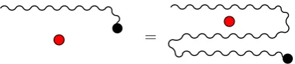
whereσ > σ0. One choice of the contours defining x− is given by the wavy line in Figure 2.2, which represents graphically the equation (2.2.14) and it is meant to reach ±∞to the right and left respectively, though the contours can be freely deformed in the absence of poles.
=
FIGURE 2.2: Braiding of currents with local fields in the world-sheet (i.e. σ-τplane, see Fig. 2.1), where we assume the lines on the left to
continue toσ = −∞and likewise those on the right to ∞. The red
vertex corresponds to the world-sheet position of the local field and the black vertex to the position of the local part of the current.
The action on the fields, ˆQIˆ[ΦA(σ0)], is given by a separate integration contour γ(σ0)starting and ending atσ = −∞which surrounds the pointσ0, represented by the solid line in Figure 2.3. This is to be distinguished from the equal time contour used to define global charges acting on asymptotic states and so we use the ˆ notation.
Correspondingly the action of the charges on products of fields, represented dia-grammatically in Fig. 2.4, can be calculated from the braiding of the current with the fields. It is explicitly given by
ˆ
QIˆ[ΦA1(σ1)ΦA2(σ2)] =QˆIˆ[ΦA1(σ1)]ΦA2(σ2) +Υˆ
ˆ
J
ˆ
[image:41.595.195.410.390.437.2]FIGURE 2.3: Integration contour (solid line) defining the action of a charge on a field, assuming that the lines on the left continue toσ =
−∞, while the wavy line is once again the integration contour defining x−.
= +
FIGURE2.4: Action of a charge on products of fields, derived from the braiding of the current with the fields.
If we think of the fields at a specific world-sheet pointΦA1(σ1)as defining a vector
spaceV1we can think of products of fields at different points, e.g.ΦA1(σ1)ΦA2(σ2)as
defining tensor products,V1⊗V2. As the world-sheet theory involves both bosonic and fermionic fields we will use a graded tensor product13
(a⊗b)(c⊗d) = (−1)|b||c|(ac⊗bd).
where|a|= 0 if the element of the algebra is even and|a|= 1 if it is odd. The action of charges on products of fields yields an operator∆(QˆIˆ)acting onV1⊗V2which in turn defines the coproduct
∆(QbIˆ) =QbIˆ⊗1+Υˆ ˆ
J
ˆ
I⊗QˆJˆ.
From the form of the currents in the world-sheet theory we have the following expres-sions for the coproduct and the braiding operator ˆΥJˆˆ
Iwhich has the non-zero elements
13At different points we use the lettersa,b,c, . . . to denote both elements of an algebraAandpsu(2|2)
{ΥˆDB
AC, ˆΥHH, ˆΥCC, ˆΥC
†
C†}given by:
∆(QAˆ B) =QAˆ B⊗1+ΥˆDBAC⊗QDˆ C, ΥˆDB
AC= δADδCB eieABP,
∆(Cˆ) =Cˆ ⊗1+ΥˆCC⊗Cˆ , ΥˆC C=eiP, ∆(Cˆ†) =Cˆ†⊗1+ΥˆCC†† ⊗Cˆ†, ΥˆC†
C† =e−iP, ∆(Hˆ ) =Hˆ ⊗1+ΥˆHH⊗Hˆ , ΥˆHH=1,
(2.2.15)
whereeAB = ([A]−[B])/2. We also have the coproduct for the braiding operator
∆(ΥˆJˆˆ
I) =Υˆ
ˆ
K
ˆ
I ⊗Υˆ
ˆ
J
ˆ
K,
or explicitly
∆(ΥˆDBAC) = ΥˆFBAE⊗ΥˆDEFC =δFAδEBeieABP⊗δFDδECeieDFP,
∆(ΥˆCC) = ΥˆCC⊗ΥˆCC=eiP⊗eiP,
∆(ΥˆCC††) = ΥˆC †
C†⊗ΥˆC †
C† =e−iP⊗e−iP, ∆(ΥˆHH) = ΥˆHH⊗ΥˆHH=1⊗1.
These follow from the simple contour argument in Fig. 2.5 and are equivalent to
∆(eimP) =eimP⊗eimP, m∈Z.
=
FIGURE 2.5: Braiding Coproduct: analyticity allows to freely deform the contour around the fields.
We will be interested in studying the algebraAgenerated by ˆQIˆand ˆΥ ˆ
J
ˆ
Ior
equiv-alently the algebra generated by the global charges QIˆ and the global braiding Υ ˆ
J
ˆ
defined by the contour fromσ = −∞to∞, which has the same coproduct. The alge-braAimplicitly comes with the multiplication mapm:A ⊗ A → Aand the identity operator id defined such that the coproduct satisfies coassociativity
(∆⊗id)∆= (id⊗∆)∆. (2.2.16)
We define the action of products of algebra elements so that the coproduct is an alge-bra homomorphism i.e. for alla,b∈ A
∆(ab) =∆(a)∆(b).
In addition to the coproduct we can equip this algebra with a counit and antipode.
The counit as vacuum expectation
The action of the counit can be thought of as the vacuum expectation of the various global operators and so we have
e(1) =1 , e(QIˆJˆ) =0 , e(ΥJIˆˆ) =δIJˆˆ. (2.2.17)
Equivalently we can define the counit as the action of the operators on the identity i.e. fora∈ A
e(a) =aˆ(1), (2.2.18)
which gives the same result. We can define the action of the generators so that the counit is also an algebra homomorphism: e(ab) = e(a)e(b)for everya,b ∈ A. This definition of the counit is consistent with the property,
(e⊗id)∆= (id⊗e)∆. (2.2.19)
The antipode as Euclidean Rotation
elementaofAthey defined an antipodesas
s(a) =Rπ(a). (2.2.20)
Even for the case of the non-Lorentz invariant world-sheet theory we can repeat this identification by defining the rotation to act on the symmetry charges by a combina-tion of time-reversal transformacombina-tion followed by a parity transformacombina-tion plus a rever-sal of the integration path defining the charge.
We first consider the action of the antipode on the symmetry charges by writing the action of the product of a time-reversal transformation followed by a parity trans-formation acting on the local part of the currentsΩAB
P T(ΩAB(σ)) =ΩAB(−σ), (2.2.21)
which can be seen explicitly at the level of the quadratic currents, see App. B. For the bosonic chargesB={Rαβ,Lab,H}this simply impliess(B) =−B. For the fermionic
currents, and for the central chargesC,C†, the issue is complicated slightly due to the presence of the zero-mode of the light-cone coordinatex−. The contour definingx−
is deformed, resulting in an additional factor:
s(QAB) =−e−ieABPQAB, s(C) =−e−iPC, s(C†) =−eiPC†. (2.2.22)
For the global (or for that matter the usual) braiding operatorsΥˆJˆ
I either rotation
sim-ply acts as P T or equivalently reverses the orientation of the contour defining x−. Hence the action of antipode gives the inverse acting on the braiding operator
ΥIˆ
ˆ
Ks(Υ
ˆ
J
ˆ
I) =δ
ˆ
J
ˆ
K. (2.2.23)
Noting that the factors such as e−iP that appear in the antipodal action on the global charges are related to the global braiding operator, we can write the action on the global charges as
s(QIˆ) =−s(Υ ˆ
J
ˆ
This is exactly the same formula as in [63]. Due to the time-reversal in the definition the action on products of elements of the algebra is
s(ab) = (−1)[a][b]s(b)s(a), (2.2.25)
where we have included the grading factor to account for the odd elements of the algebra and thus we note that the antipode is an antihomomorphism. We also have the trivial action of the antipode on the identity element, i.e. s(1) = 1. Indeed for any operator which commutes with the world-sheet momentum, which includes all of the braiding operators and all the global charges, we do have s2(a) = a. It is straightforward to check that the world-sheet antipode satisfies
m(s⊗id)∆=m(id⊗s)∆=1e. (2.2.26)
We also note that due to the time reversal in the definition of the antipode we have that
∆(s(ΥJˆˆ
I)) =s(Υ
ˆ
J
ˆ
K)⊗s(Υ
ˆ
K
ˆ
I). (2.2.27)
In fact, this relation is trivial, since the matrix structure of the braiding factors is es-sentially trivial. However, writing it in this way makes it straightforward to show the identity
∆s= (s⊗s)∆op (2.2.28)
where∆op = P∆with P(a⊗b) = (−1)[a][b](b⊗a)is the skew comultiplication. We can use∆opto define the skew antipodes0as
m(s0⊗id)∆op=m(id⊗s0)∆op =1e. (2.2.29)
Following [63], we can think of this from the world-sheet perspective as a rotation in the opposite direction to s, i.e. s0 = R−π. The identity (2.2.29) is consistent for the
world-sheet theory as
s0(QIˆ) =−QJˆs0(ΥJˆˆ
I) and s
0(ΥKˆ ˆ
I)Υ
ˆ
J
ˆ
K= Υ
ˆ
K
ˆ
Is
0(ΥJˆ
ˆ
K) =δ
ˆ
J
ˆ
This definition gives the natural relationss0 =s0s=1.
2.2.4 Adjoint actions
Essentially everything above is well known for the world-sheet theory. As we are interested in studying form factors and their generalizations, we wish to understand the action of the symmetries on the fields of the theory as well as on asymptotic states. This requires the generalization of the commutator of global charges to the adjoint action of a quantum group [62, 63]. Given an element of the algebraa ∈ A, we can define further elements of algeb