u 1L
D. Conniffe
and
S. ScoH
a
THE ECONOMIC & SOCIAL RESEARCH INSTITUTE
THE ECONOMIC AND SOCIAl., RESI’ARCH INSTITUTE COUNCIL
*TOMAS F. O COFAIGH, LL.D., President of the Institute.
*EUGENE McCARTHY, M.Sc.Econ., D.Econ.Sc., Chairman of the Council. K. BONNER, Secretary, Department of Labour.
V.K. BOROOAH, M.A., Ph.D., Professor, Department of Applied Economics and Human
Resource Management, University of Ulster at Jordanstown.
J. CAWLEY, Senior Partner, Cawley Sheerin I+l/ynne.
L. CONNELL:\N, B.E., C.Eng., M.I.E.I., Director General, Confederation of Irish
Industry.
*SEAN CROMIEN, B.A., Secretao,, Department of Finance.
MICHAI’2L P. CUDDY, M.Agr.Sc., Ph.I)., Professor, Department of Economics,
UniversiO, College, Gahoay.
*MARGARET DO\VNES, B.Coram., F.C.A., LI..D., Director, Bank of Ireland. *MAURICE 1". DOYI.,E, B.A., B.[.., Governor, Central Bank of Ireland.
DERMOT EGAN, Director, Allied Irish Banks plc. P.\V. FLANAGAN, Dublin.
PATRICK A. HALL, B.E., M.S., Dip.Slat., Director of Research, Institute of Public
Administration.
*KIERAN A. KENNEl)Y, M.Econ.Sc., D. Phil., I:’h.D., Directo~of the hlstitute. T.P. LINI’2HAN, B.E., B.Sc., Director, Central Statistics Offce.
P. INNCH, M.A., M.R.I.A., Dublin.
*D.F. McALI’2ESE, B.C, omm., M.,’\., M.Econ.Sc., l:’h.D., Whately Professor, Department
of Economics, Trinity College, Dublin.
E.F. McCUMISKEY, Secretary, Department of Social H/elf are.
.JOHN J. McKAY, B.Sc., D.P.A., B.Comm., M.Econ.Sc., Chief Executiue Officer, Co.
Cavan Vocational Education Committee.
*D. NEVIN, Dublin.
.JOYCE O’CONNOR, B.Soc.Sc., M.Soc.Sc., Ph.l)., Director, .A’?ttional College of
Industrial Relations, Dublin.
LEO O’DONNELL, Managing Director, Irish Biscuits plc.
MAURICE O’GRADY, M.Sc(MGMT), Director General, h’ish Management Institute. \V.G.H. QUIGLEY, Ph.I)., (;hairman, Ulster Bank, Ltd.,
PIERCE RYAN, B.Agr.Sc., M.Sc., Ph.I)., M.R.I.A., Director, Teagasc.
S. SHI~+I:+H~ , B.Agr.Sc., Ph.D., Professor, Department of Applied Agricultural Economics.
UniversiO, College, Dublin.
.J.SI:’ENCER, B.Sc. Econ., Proj~ssor, Department of Economics, 7"he Queen’s University.
Belfast.
*B.M. WALSH, B.A., M.A., Ph.l)., Professor, National Economics of Ireland and Applied
Economics, University College, Dublin.
REV. C.K. WARD, B.A., S.T.[..., Ph.D., Professor, Department of .Social Science.
Universi9, College, Dublin.
*T.K. WHITAKER, M.Sc.Econ., D. Econ.Sc., LL.D., Dublin.
*P.A. WH[TE, l].Comm., I).P.A., Director, Dresdner International Finance plc.
ENERGY ELASTICITIES:
RESPONSIVENESS OF DEMANDS FOR
FUELS TO INCOME AND
PRICE CHANGES
Copies of this paper may be obtained from The Economic and Social Research Institute (Limited Company No. 18269) Registered Offce: 4 Burlington Road, Dublin 4
Price 1111£ 10.00
ENERGY ELASTICITIES:
RESPONSIVENESS OF DEMANDS FOR
FUELS TO INCOME AND
PRICE CHANGES
D. Conniffe
and
S. Scott
© THE ECONOMIC AND SOCIAL RESEARCH INSTITUTE DUBLIN, 1990
Acknowledgements
The authors would like to express their gratitude to all those who have made this study possible. Preliminary research, on which this publication is partly based, was commissioned by BGE, the Department of Energy and the ESB. Assistance with data was provided by Bord Gais Eireann, Bord na Mona, the Central Statistics Office, the Department of Energy, Dublin Gas, Electricity Supply Board and several oil companies. Our thanks go to our colleagues John Bradley and John Fitz Gerald for their comments on earlier drafts of this paper and to an anonymous external referee. Useful comments were also received from staff of the Central Bank on a penultimate version. Finally, we would like to thank the clerical staff of the ESRI for processing the various drafts of the paper, Pat Hopkins
for help with artwork and Mary McElhone for preparing the manuscript for publication. The authors are, of course, solely responsible for the final document and any errors or omissions which remain.
Chapter 1 l.l 1.2 1.3 2 2.1 2.2 2.3 2.4 3.1 3.2 3.3 3.4 4 4.1 4.2 ’t-.3 4.4 Acknowledgements General Summary INTRODUCTION
The Motivation for this Study The Scope of this Study Content of Future Chapters
DATA SOURCES
Introduction
Time Series Data 1960-1987 Average versus Marginal Prices Household Budget Survey Data
MODELS FOR INDIVIDUAL FUELS: TIME-SERIES AaVALTSIS
Introduction
An Expenditure Shares Model Quantity Equations
Elasticities
THE AGGREGA TE ENERGY MODEL
Introduction
The Diminishing GDP Elasticity Lagging Effects
Otller Modified Models
Chapter 5
5.1 5.2
5.3 5.4
5.5
6 6.1 6.2 6.3
INCOME ELASTICITY ESTIMATES FROM HOUSEHOLD BUDGET SURVEY DA TA
I ntroductlon
Data for Analysis, Definition of Income and Grouping of Households
Choice of Curves and Elasticity Estimation Estimated Equations and Elasticities Energy Using Appliances
CONCLUSIONS AND DL~CUSSION
Summary of Results on Elasticities Comparison with Other Estimates
Using the Elasticities
References
Page
48 48
49 55 62 67
72 72 75 77
79
Tab& 2.1 2.2 2.3 2.4. 3.1 3.2 3.3 3.4. 3.5 3.6 3.7 3.8 3.9 3.10 4.1 4.2 4.3 4.4 5.1
End Users’ Consumption of Fuel in MTOE
Prices of Fuels at End-use, £ per TOE
Correlations Between Deflated Fuel Prices
Relative Shares of Fuels in 1960 and 1987
Regression Regression Regression Regrcssiou Regression Regression Individual Results
Results for Gas
Results for Electricity
Results for Coal
Results for Turf
Results for Oil
Resuhs for LPG
Fuels -- Regression Equation
Modified Individual Fuel Equations
Elasticities of Fuels with Respect to GDP
Own and Cross-price Elasticities for the Fuels
Elasticities from the Split Sample
Elasticities
Elasticities
Elasticities
Household
from Variable Elasticity Model
of Modified Models
of Other Modified Models
Budget Survey 1987 -- Summary Data
Table
5.2
5.3
5.4
5.5
5.6
5.7
5.8
5.9
5.10
5.11
5.12
5.13
5.14
5.15
5.16
6.1
6.2
Page
Central Heating in 1987 -- Percentages of
Households 51
A Comparison of 1980 and 1987 for Gas-connected
Households 52
Central Heating 1980 and 1987 -- Percentages of
Gas-connected Households 52
Gross Incomes at Mean Expenditure of Urban
Households in 1987 HBS 53
Explanatory Power (R~) of Alternative Curves
(Gas-connected Households) 61
Coefficients and Standard Errors, 1987 62
Regression Analyses for Gas-connected
House-holds, 1987 63
Comparison of Standard Errors of Unweighted
and Weighted Regressions 63
Elasticities at Mean Income, 1987 64
Regression Coefficients for Both Income and
Household Size, 1987 66
A Comparison of Elasticity Estimates for Irish
Data 67
Income Coefficients and Income Elasticities
Controlling for Central Heating, ,1987 67
Percentages of Types of Central Heating by
Income Group -- Urban Households 1987 68
Percentages of Types of Central Heating by
Income Group -- Gas-connected Households 1987 69
Electricity Elasticities 1987 71
Own and Cross-price Elasticities for the Fuels 73
Elasticities at Mean Income 1987 from HBS Data 75
2.1 2.2 2.3 2.4 2.5 2.6 2.7 2.8 4.1 4.2 4.3 5.1 5.2 5.3 5.4 5.5 5.6 5.7
Deflated Price of Gas
Deflated Price of Electricity
Deflated Coal Prices
Deflated Turf Prices
Deflated Price of Oil
Deflated Price of LPG
Real GDP 1960-1987
Total Energy (MTOE) 1960-1987
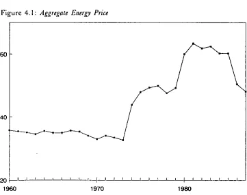
Aggregate Energy Price
Residuals from Constant Elasticity Model
Residuals from the Variable Elasticity Model
Plausible Fuel Expenditure[Income Relationship
Total Energy Expenditure (£]week) in 1987 Gas-connected Households
Gas Expenditure (£]week) in 1987 Gas-connected Households
Electricity Expenditure (£/week) in 1987
Gas-connected Households
Expenditure on Coal (.~’/week) in Gas-connected Households
Expenditure on Oil (~/week) in Gas-connected Households
Index of Selected Electrical Appliances, 1987
GENERAL SUMMARY
In the last two years economic commentators generally reached favourable views about the likely prospects for the Irish economy in the medium term. For example, the ESRI’s (1989) "Medium-Term Prospects
for lrelaud" (Bradley and Fitz Gerald, 1990) forecast that for 1989-1994 the average annual growth rate of real GNP would be 4 per cent, with GDP growth even larger. Increased growth implies a greater demand for energy, but how mucb greater? How will the increased demand break down by fuel and what role will relative prices play? However, this study is not aimed at providing specific forecasts for fuel requirements, because these are at best only as good as the forecasts for GDP and for world energy prices. Indeed, since this study commenced there have been dramatic developmcnts in Eastern Europe, the US and UK economies have experienced difficulties, and there is a threat of war in the Middle East. Very recent economic forecasts have been highly tentative.
Instead, this study estimates fuel elasticities with respect to GDP and to fuel prices. The GDP elasticity is the percentage increase in demand for fuel, given a I per cent increase in GDP. The price elasticities are the percentage decrease (or increase) in demand for a fuel, given a per cent increase in its own price (or rival fuel price). These elasticities, deriving from relationships observed over time, are much more likely to be stable, at least in the medium term, than GDP projections. Once estimated, the elasticities can be applied to whatever projections are currently favoured and indeed application to a range of scenarios may have value in helping to assess the required response of lrcland’s energy infrastructurc to alternative developments.
elasticities for GDP and price are estimated at aggregate level from the time-series data. There are, however, detailed data on the household sector contained in the Household Budget Survey and these are used to c;stimate "income" elasticities. Actually "income" is defined as total household expenditure to circumvent the notorious difficulties associated with measurement of income in surveys. Unfortunately the rounds of the Household Budget Survey are only conducted at seven year intervals, so that information on price variation through time is lacking. So "income" elasticities can be estimated for the domestic sector, but not price elasticities.
Before the oil crisis of the 1970s, GDP elasticities were reported in various international studies as generally exceeding unity and by considerable amounts in the case of developing countries. That is, every extra 1 per cent of economic growth required a greater than 1 per cent increase in the energy input. Recent studies in the international literature have strongly suggestedthat GDP elasticities have dropped substantially since then, especially in the developed countries. Writers have not been unanimous on the extent of the decrease, or on precisely why it has occurred, but the majority opinion is that economic growth is now a lot less energy intensive than it used to be.
One reason is that severe price rises for energy, besides depressing demand directly, trigger major research into more energy efficient
technology. Even when prices fall again, that technology remains in place, so that the increase in energy use following a price fall does not match the previous decrease. So instead of appearing as a large and reversible price effect, the phenomenon appears as an irreversible decrease in the
GDP elasticity. However, this is not the only explanation for diminishing GDP elasticities. Economies may evolve through stages of differing energy intensity and a change of main growth areas from manufacturing to services will have implications for energy requirements.
Returning to the Irish situation, this study finds that the GDP elasticity for aggregate energy declined fi’om a pre-oil crisis value of about 1.3 to a current value of just less than .5. That is, energy demand has changed from a state of being elastic with respect to GDP to one of being quite inelastic. Aggregate energy is made up from the fuels: gas, electricity, coal, turf, oil and LPG. Of these, neither coal nor turf showed any significant relationship with GDP over time, ahhough in interpreting this it is important to remember the "final demand" definition of fuel quantities. The current elasticities for gas, electricity, oil and LPG are .48, .58, .20
GENERAL SUMMARY 3
Turning to price effects, the own price elasticity of aggregate energy was estimated at being --.21, which is quite an inelastic figure. So a 10 per cent increase in aggregate energy price would produce only a 2 per cent decrease in energy demand. However, it does not follow that the own price elasticities of individual fuels all have to be small. An individual fuel could have a high own price elasticity, in that other fuels might quickly replace it in the aggregate mix if its price rose independently of other prices. Statistically significant own price elasticities were found for all fuels except turf and LPG. The elasticities were less than l for
electricity and oil and greater than I for gas and coal. The high figures suggest considerable price sensitivity, but may also reflect energy policy measures on natural gas and the early 1980s grants for installing coal burning equipment.
Most cross-price elasticities were not found statistically significant, but some were. No other fuel showed a significant cross-elasticity on electricity price and although electricity demand did show statistically significant relationships with gas, turf and oil prices, the elasticities were small.
Generally, this suggests that the scope for substitution away from electricity to other fuels is small. On the other hand, some cross-elasticities were large. Gas showed a cross-elasticity of just over unity with LPG price and coal had a cross-elasticity of near unity with oil price and a surprisingly large cross elasticity with turf price. Coal appears a price sensitive fuel in all respects. Smaller elasticities included those for gas on coal price, oil on gas price and coal on gas price. The last mentioned is a little puzzling since it is negative, as indeed was the small electricity on gas price elasticity. Gas is rather special among the six fuels in that the change in the early 1980s from manufactured town gas to natural gas was accompanied by far reaching changes. Previously, gas had been primarily a domestic fuel with a limited gas grid, competing with electricity for cooking and with coal for heating. Afterwards, gas increased its role as an industrial fuel competing with oil and LPG, as well as challenging oil as a central heating fuel in the domestic sector.
The "income" elasticities outlined for the household budget survey data need not be directly comparable with the GDP elasticities already
Chapter 1
INTRODUCTION
1.1 The Motivation for this Study
Comparatively recent assessments of the state of the Irish economy have
painted fairly bright pictures of the prospects for future growth. For example, the ESR[’s "Medium Term Prospects for Ireland"(Bradley and Fitz Gerald, 1990) forecast that for 1989-1994 the average annual growth rate of real GNP would be 4 per cent, with GDP growth even larger. Obviously increased growth implies a greater demand for energy, but how rnuch greater? How will tile increased demand break down by fuels and what role will relative prices play? If the GDP elasticity -- the percentage increase in demand for a fuel, given a 1 per cent increase in GDP -- and the price elasticities -- the percentage decrease (or increase) in demand for a fuel, given a I per cent increase in its own price (or rival fuel price) -- are known, these questions can be answered.
The reasons why it is important to have answers are easily stated and some are perhaps almost self-evident. Energy is essential for the functioning of every sector of the economy and, indeed, GDP forecasts implicitly assume tile availability of adequate suppfies in appropriate forms. Fuels
difl’er in the lead time required to make increased volumes available. For electricity, there can be a gap of several years between deciding on extra
generating capacity and having it available. It is true that the over-optimistic estimates of economic growth and consequent demands for electricity, that were made in the 1970s, were partly responsible for the excess capacity during most of the 1980s. But that situation might not continue. Breakdowns between fuels are also important because of varying import contents and, nowadays, also because of differing environmental impacts.
Firms in the fuels industries can use elasticities to help deduce the
implications for their markets of forecasts of economic growth or price movements. If government wishes to implement an energy (or environmental) policy, then its advisers can use elasticities to assess the effectiveness of such instruments as taxes and subsidies. Even at the level
relevant sections of the European Commission, elasticities are required to provide the detail requested. In fact, this ESRI paper has grown out of an unpublished report (Conniffe, 1989) commissioned by Bord Gais Eireann, the Department of Energy and the Electricity Supply Board. The brief for that project was to estimate elasticities using whatever data were reasonably accessible at the time. This work draws heavily on that report as regards econometric methodology and estimates, but builds into a framework of previous Irish research on energy elasticities and on the material in the international literature.
1.2 The Scope of this Study
Over the years, the ESRI has made substantial contributions in the area of Irish energy economics. Booth (1966a, 1966b, 1967a, 1967b) and
Scott (1978-79, 1980) looked at the energy scene in the 1960s and late 1970s, respectively. Elasticity estimation was part of their work, but they went on to actual forecasting of future demand and commenting on various aspects of energy policy. Similarly Henry (1976, 1983) treated econometric estimation as just a step in broader, policy oriented studies.
This paper is much more limited in scope in that context. It deals with the estimation of elasticities and the technical issues that arise in the process. This is not to say that the authors do not think it important that a broader study be conducted. Indeed, the likelihood that the Irish economy is currently at a turning point makes such a study most desirable. But previous Irish researchers had not as much data as are currently available; not that what is now available could be considered excessive. Booth had to rely on international comparisons to a large degree, since there was so little Irish data, and Scott concentrated on aggregate energy rather than on individual fuels. In addition, especially in Booth’s case, the hardware and software for fairly sophisticated statistical analyses were just not available. So the volume of econometrics was limited in the past, but now has grown sufficiently to constitute an ESRI paper in itself.
The extension to full forecasting of energy would require critical examination of the GDP and price projections to which the elasticities would be applied and assessment of the models and assumptions from which they were derived. Inevitably, such projections are highly tentative and can be subject to re-evaluation whenever previously unforeseen
political or economic developments affect the international or national scene. Indeed, since this study commenced, there have been the dramatic developments in Eastern Europe and now the possibility of war in the
I NTRODU G’TION 7
from the relationships observed over time between quantities, GDP, and prices, are more likely to be stable and can be applied to alternative projections, so there is value in providing the elasticities on their own. Further broadening of scope towards analysis of energy and environmental policies, while undoubtedly very useful, would lead to an excessively long publication. So, for example, the important current developments as regards pollutant emissions are not explicitly considered in this report.
1.3 Content of Future Chapters
Chapter 2 will describe the data to be employed in the analyses. Most attention will be given to describing an in-house dataset that has been accumulated on individual fuel quantities and prices. An earlier version
of the dataset was used by Scott in the papers already referred to. While the dataset is now reasonably comprehensive at national aggregate level, it is unfortunately not currently possible to disaggregate to sectoral level. One source of information on the domestic sector is the Household Budget Survey, as published by the Central Statistics Office and use will be made of its data.
The individual fuel elasticities with respect to GDP and prices are investigated and estimated in Chapter 3. An expenditure shares model, of a type frequently appearing in the international literature, is first fitted to the data, but later replaced b); a more pragmatic approach. Aggregate energy is examined in Chapter 4 and elasticities with respect to GDP and
a nleasure of aggregate price are estimated. The cross-sectional type data from budget surveys are analysed in Chapter 5, taking account of various household characteristics and possessions, especially the effects of possession of various types of central heating. Comparisons are also made with the estimates obtained by previous researchers.
DA TA SOURCES
2.1 Introduction
Few researchers ever have as adequate datasets as they would like and the situation with regard to Irish energy data -- both quantities and prices -- is particularly difficult. As mentioned in the introductory chapter, the authors have data at national level on quantities and prices of fuels based on time series compiled at tile ESRI from a variety of sources. It would be better to have reliable data broken down by sector and the theme of more desirable data will I~e mentioned again in later chapters. However, this chapter will describe the data that are available and discuss related issues.
As was also mentioned in Chapter 1, income elasticities for the domestic sector can be estimated from a cross-section of households and relevant data are available from tile Household Budget Survey (HBS), which is conducted by the Central Statistics Office. Since the HBS is a well known survey, documented in CSO publications, only a brief account will be given in this chapter.
2.2 Time Series Data, 1960-1987
There are several partially overlapping sources of information on energy consumption and energy prices. These include Booth (1966a; 1966b; 1967a; 1967b), OECD (1974; 1975; 1976) and the Department of Transport and Power, now the Department of Energy. However, anyone who has tried to reconcile some of the divergent figures, to produce a 20-or 30-year time series, knows that at best they can only obtain an
DATA SOURCES 9
treated separately in the analyses in subsequent chapters. There are other fuels, for example timber, but quantities are small and comprehensive data are unavailable.
The term "end user" means that fuels delivered to other fuel processors
were excluded, for example: oil or gas used in electricity production. Fuels for non-energy use, such as feedstock for the chemical industry are also excluded. Fuel quantities were taken from OECD sources until 1974 and from the Department of Energy’s publication Energy in Ireland for the
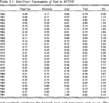
subsequent years. The Department’s figures actually go back to 1972, but the two series were in much closer agreement in 1974 than in the previous two years. All quantity data were converted into the common units of TOE (tonnes of oil equivalent) using the appropriate conversion factors. There are some complications. Hand won peat, as distinct from commercial peat production, had to be added in from the CSO’s data on agricultural output in the Irish Statistical Bulletin. Since there is no information available on stocks held by households or firms, the consumption quantities are gross of stocks. With annual data this ought not to be a problem, but it is possible that just after each oil crisis, stock build-ups occurred. The quantities of fuels are shown in Table 2.1.
Turning to prices, it must be stressed that the aim was to have a time series of broadly representative prices. For electricity, units sold and revenue from sales were taken from the appendices to ESB annual reports. The data referred to financial years, but were converted to calendar year pro rata time. The authors appreciate that there have been objections raised in the energy literature to use of this type of "average" price rather than to use of a "marginal" price, but will treat the issues in the next section. In any event, the need to treat fuels on a reasonably similar basis and the impracticality of obtaining anything except an average price for all fuels left little alternative.
The price of Dublin gas was used for the years before the arrival of natural gas and a weighted average of Dublin Gas and Bord Gais industrial prices was used thereafter. For coal, price data for 1960 to 1971 were derived by the CSO from the consumer price index and from 1971 on these were obtained from Bord na Mona, who collect data on fuels competing with turf.
Table 2.1: End-Users’ Consumption of Fuel in MTOE
Total Gas Electridty Coal Turf Oil
1960 0.08 O. 17 0.86 O. 78 0.90
1961 0.08 O. 17 0.97 0.81 I. 14
1962 0.08 0.19 0.85 0.83 1.3 I
1963 0.09 0.20 0.87 0.80 1.24
1964 0.10 0.24 0.80 0.73 1.44
1965 0.10 0.26 0.76 0.70 1.62
1966 0.10 0.29 0.81 0.73 1.84
1967 0.12 0.32 0.80 0.64 2.10
1968 0.11 0.35 0.80 0.64 2.18
1969 0.14 0.38 0.75 0.61 2.70
1970 0.16 0.41 0.72 0.60 2.95
1971 0.17 0.45 0.63 0.62 3.59
1972 0.19 0.49 0.56 0.62 3.65
1973 0.21 0.53 0.49 0.65 4.09
1974 0.22 0.55 0.47 0.57 3.78
1975 0.21 0.54 0.37 0.57 3.50
1976 0.22 0.58 0.43 0.60 3.52
1977 0.23 0.63 0.46 0.62 3.77
1978 0.24 0.68 0.50 0.59 3.84
1979 0.30 0.75 0.78 0.60 4.12
1980 0.31 0.75 0.75 0.58 3.87
1981 0.32 0.74 0.84 0.59 3.71
1982 0.33 O. 74 0.84 O. 73 3.43
1983 0.31 0.78 0.97 0.69 3.22
1984 0.40 0.80 0.96 0.71 3.16
1985 0.48 0.85 1.02 0.73 3.12
1986 0.57 0.89 1.18 0.65 3.18
1987 0.62 0.91 1.06 0.66 3.14
and involved weighting for bagged peat and briquettes and so on. The prices of the main petroleum products, namely motor spirit, gas oil and fuel oil, were weighted by sales quantities to give an aggregate oil price. The source of price data was a major oil company and the quantity weights were derived from Booth (1966a, 1966b) for 1960-1963, from
Energy in Ireland for the post-1972 years and by interpolation for the
intervening years. The price calculations were complicated by the fact that there were sometimes numerous price changes within a year, necessitating further weighting by the number of months a particular price was charged.
DATA SOURCES I 1
imports. Because of the confidentiality issue, the prices of gas and LPG will be combined by weighting them by quantity.
[image:22.506.69.425.187.509.2]The account given, with its references to interpolation and estimations, shows the difficulties inherent in assembling good energy price data over a long time series. The prices are shown in Table 2.2 and are expressed in Irish £s per TOE.
Table 2.2: Prices of Fuels at End-use, £ per TOE
Total Gas Electricity Coal Turf Oil
1960 47.1 101.3 10.9 13.3 34.5
1961 46.6 102.3 12.1 13.5 33.9
1962 47.8 101.3 13.0 14.4 32.2
1963 48.3 100.2 14.0 14.6 31.6
1964 49.5 100.6 15.4 14.6 33.0
1965 49.3 98.0 15.3 14.8 33.4
1966 52.4 98.2 15.3 15.9 33.9
1967 51.0 99.6 15.8 16.8 34.4
1968 52.1 101.8 16.5 16.8 35.3
1969 53.1 105.4 17.7 16.6 35.0
1970 54.2 109.7 20.2 18.2 35.2
1971 57.9 117.9 22.7 20.3 39.7
1972 62.8 127.1 27.5 21.6 40.4
1973 67.5 142.1 29.6 23.7 41.6
1974 100.7 205.2 50.4 29.1 68.3
1975 125.0 250.6 55.8 35.3 93.8
1976 138.8 286.3 58.2 37.7 119.1
1977 161.9 324.2 76.5 43.0 135.9
1978 170.2 327.3 83.9 47.8 136.5
1979 180.2 387.0 96.4 58.9 162.5
1980 269.0 528.3 126.6 77.8 239.6
1981 348.0 662.7 153.5 93.5 313.2
1982 366.8 759.2 163.0 93.3 376.8
1983 376.5 823.6 165.0 100.4 436.2
1984 351.2 864.4 184.5 99.3 459.0
1985 338.1 893.0 220.2 119.6 484.8
1986 245.7 883.1 212.9 126.4 386.8
1987 228.7 815.1 203.3 119.9 395.5
Figure 2. l: Deflated Price of Gas
80
4O
0 I I I k i ~ I i I I I I I P I I I i I ’, J ~ I I i I
1960 1970 1980
Figure 2.2: Deflated Price of Electricity
160
120
DATA SOURCES 13
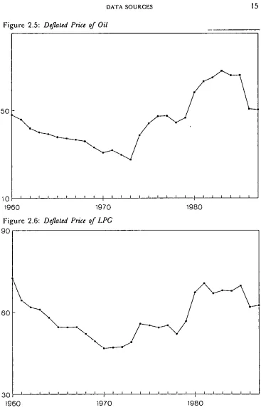
Tile corresponding growth for electricity price is shown in Figure 2.2. Up to the first oil crisis in 1974, both graphs show a steady decrease in real prices, more pronounced for electricity than gas, followed by steep increases, gradual decreases until the second oil crisis in 1979 when further steep increases occurred. Subsequent prices decreased again, most dramatically so for gas, with the price reduction associated with the conversion to natural gas. Figure 2.3 shows the evolution of coal prices. While there was no decrease before the first oil crisis, there was a stability of price followed by increases associated with the oil crises and an eventual price decrease. However, the decrease is not as pronounced as with gas or electricity. The turf price growth is shown in Figure 2.4. For this fuel an initial price decline was followed by a more or less stable low price which persisted longer than for the fuels already described. Prices have stabilised in recent ),ears. The graph for oil price is shown in Figure 2.5 and the influences of the two oil crises are very evident. The graph for LPG is "shown in Figure 2.6. While of generally similar shape to the oil price curve, the initial decline in the 1960-1974 period was from a relatively higher starting level than for oil and fell further. Indeed, LPG real prices never reached as high a level as they started from in 1960. Of course, the quantities of LPG were relatively small in 1960.
35
2O
Fi ure 2.3: Deflated Coal Prices
It is postulated that demand for a fuel depends on GDP and on prices
-- its own price and the prices of other fuels that might substitute for it.
Obviously enough, some fuels are more easily substituted for than others and to greater degrees. One obstacle to measuring price substitution effects
[image:25.506.71.437.241.605.2]using time series data can be that all the prices move together over time, that is, there is little relative price variation. To check on this point the pairwise correlation coefficients of deflated prices were calculated and are given in Table 2.3.
Table 2.3: Correlations Between Deflated Fuel PHces
Gas Electddty Coal Turf Oil LPG
Gas 1.00 .43 -. 16 .52 -- .05 .69 Electricity .43 1.00 .22 .51 .68 .88 Coal -.16 .22 1.00 -.25 .70 .41 Turf .52 .51 - .25 1.00 - .04 .34 Oil -- .05 .68 .70 - .04 1.00 .86 LPG .69 .88 .41 .34 .86 1.00
Figure 2.4: Deflated Turf Prices
2O
10 I 1960
Ilrl
DATA SOURCES [ 5
50
Fiure 2.5: Deflated Price of Oil
[image:26.495.59.426.63.646.2]1960 1970
Figure 2.6: Deflated Price of LPG
I I I
30 I i t I t I I I I l--t I ~ I I i I ? r [ I P I I I I
In general, the correlations, while occasionally high, are not so large as to preclude good estimates of cross-price effects, assuming these exist. In fact, the correlations of gas price with some other fuel prices are actually negative. This is because of the introduction of low priced natural gas in recent years. The correlations of oil price, LPG price and electricity price with each other are all on the high side, which may have to be borne in mind when interpreting results later.
h may be worthwhile briefly summarising the relative positions of the various fuels in 1960 and 1987. This is illustrated in Table 2.4. Looking first at quantity shares: oil, electricity, gas and LPG increased their shares between 1960 and 1987 while coal and turf decreased theirs. For expenditure, or cost, shares the picture is a little different. The oil, electricity and LPG increases are less dramatic, while gas decreased its expenditure share, which reflects big reductions in real gas prices. In general, quantity and cost shares were much closer together in 1987 than in 1960. In 1987 the cost share of electricity was about twice its quantity share, while it had been almost four times it in 1960. Again, the cost and quantity shares shown for oil were almost equal in 1987, while the cost share was nearly a third greater in 1960.
Table 2.4: Relative Shares of Fuels in 1960 and 1987
Quantity Share Cost Share 1960 1987 1960 1987
Gas .025 .073 .044 .027 Electricity .061 .142 .239 .306 Coal ,307 ,166 .130 ,089 Turf .280 .103 .144 .033 Oil .322 .491 .432 .513 LPG .005 .024 .01 I .031
Besides prices, real GDP (in £ billions at 1978 prices) will be the main explanatory variable in subsequent analyses and its growth over the period is shown in Figure 2.7. Some other variables, including population, are candidates for a role as explanatory variables, but variables highly correlated with GDP are of little use. This point will be returned to
subsequently.
DATA SOURCES l 7
discussed in the introduction to Chapter 4. The growth of aggregate or total energy, as here defined, is shown in Figure 2.8.
2.3 Average versus Marginal Prices
The prices described iu the last section were estimates of the average prices holding for a particular fuel in a particular year. It has been argued, usually in the domestic sector context and with particular reference to electricity, that average prices are less appropriate than marginal prices. The idea is that a householder will usually be faced with a schedule of prices, where the per unit price often falls with quantity, and will base decisions on the marginal price. Taylor’s (1975) criticisms of average price are probably the best known.
Fi ure 2.7: Real GDP 1960-1987
10
5
[image:29.495.75.441.74.651.2]1970 ~980
Figure 2.8: Total Energy (A4TOE) 1960-1987
8
6
i I I I I I I [ f I--I I I I I I I _ [ ~
DATA SOURCES 19
2.4 Household Budget Survey Data
The other data source mentioned in Chapter l was the 1987 Household Budget Survey. Since prices are effectively constant for a particular survey date, the 1987 survey can be used to estimate income elasticity, but not price elasticities. Unlike the situation for other countries, budget surveys in Ireland have been conducted very intermittently so that it is not possible to build up extensive time series data from them. Since the foundation of the State only six large scale Household Budget Surveys have been conducted: in 1951-52, 1965-66, 1973, 1980 and 1987. A very limited survey was conducted in 1922 and a small scale annual survey operated in urban areas only from 1974 to 1981 inclusive. Data on fuel quantities and prices for the domestic sector suitable for the estimation of price elasticities cannot be pieced together from these sources alone. Aggregate data similar to those described in the previous section for the national level should be obtainable, but much difficult and tedious estimation and interpolation would be required. Some fuels are more easily treated than others -- electricity data being the most accessible. However, the current situation is that lengthy time series exist for individual fuels only at national level.
So the 1987 round of the HBS will be employed for determining income elasticities. So will the 1980 round, for purposes of comparison with estimates from 1987 and with those obtained by researchers who examined earlier rounds. Relevant details of the survey data will be given in Chapter 5, along with the estimates, but general accounts of the rounds of the survey seem redundant given the detailed CSO publications on the subject
MODELS FOR INDIVIDUAL FUELS: TIME-SERIES ANALYSES
3. I Introduction
When the reasons for undertaking this study were outlined in Chapter I, the desirability of having detailed data for different sectors of the economy was discussed. Best of all possibilities would be to have, for each sector, an annual time series of cross-sectional micro data on fuel consumptions, prices and other influential variables. Such data exist in the UK for the household sector because the Family Expenditure Survey, the UK equivalent of the Irish Household Budget Survey, is conducted annually. But, as already explained, in Ireland the HBS is conducted only at long intervals, so that combination of data over surveys is unrealistic.
The next best situation would be to have data on annual aggregate consumptions of fuels for each sector. Then models could be fitted for each sector using the time variation in prices to estimate price elasticities and elasticities with respect to the most relevant other variables. For example, average disposable income would be relevant for the household sector, while output would be appropriate for the industrial sector. Other specifically relevant variables could probably be used to improve the plausibility and forecasting performance of the sectoral models. However,
as evident from Chapter 2, the data currently available are not sufficiently disaggregated so that such sectora] models are not yet feasible. Not only does this mean that findings will be at a more aggregated level than is desirable, but the aggregate model itself may not be fully satisfactory in fit and performance. Relating aggregate energy consumption to GDP can hardly match the explanatory power of sectoral models incorporating disposable income, industrial output, etc., and aggregate price variations may not have uniformly matched sectora[ patterns. However, the data that will be analysed in this chapter and the next are the best available.
As already described in Chapter 2, aggregate national quantities (in MTOE) and national average prices are available for the six fuels, gas, electricity, coal, turf, oil and LPG for the years 1960-1987 inclusive. Quantities will be treated as dependent variables, as will expenditure shares in some analyses, and will be related to (deflated) prices and to
MOI)ELS FOR INDIVIDUAL FUELS: TIME SERIES ANALYSES 21
real GDP. In spite of the reservations just expressed about the data,
previous Irish researchers, who have estimated energy elasticities, h’ave suffered from even greater data deficiencies. Several of these, including O’Riordan (1974--75), McCarthy (1977) and Conniffe and Hegarty (1980), were really interested in systems models of the broad commodities of consumer expenditure available in the CSO’s National Income and
Expenditure booklets. So they worked with one single composite measure of
fuels, the commodity "Fuel and Power". Scott (1978-79, 1980) possessed data on national quantities of the various types of fuel, but had to treat price indices obtained from a limited selection of fuels applying nationally. Henry (1983) and Reifly (1986) used the CSO’s Trade Statistics of Ireland to determine quantities and price indices for imported fuels and excluded domestically produced fuels from their analyses.
3.2 An E.~penditure Shares Model
This model originated with Fuss (1977) and Pindyck (1979) and was originally applied to industrial sectors, assuming that energy was weakly separable from other inputs. Assuml)tions of homothetlcity, adequacy of a trans-log flexible functional form and application of duality theory, lead to a unit cost price function for aggregate energy
log P,, = A,. + ~ Ailog Pi + ~ ~] b,j log P, log Pj, (3.1)
i i j
where the Piare the prices of the individual fuels. Application of Shepherd’s [emma leads to the expenditure share equations for the fuels
Si = A~ + ~ bu log Pj, (3.2)
J
where S~is the share of total energy expenditure spent on fuel i. Since the coefficients in (3.2) are also in (3.1) the estimation of the share equation also provides the information required to construct an aggregate energy
price. The one unknown constant Ao need not cause any difficulty since it will cancel out of an index. This way of arriving at an aggregate energy
price by actually estimating an energy aggregator, which can be claimed to be at least an approximation to a true aggregator, is often argued to he more satisfactory than simply weighting up the individual prices by quantity shares. This is because it is the unit cost under the assumption that agents are optimisers. Since shares must sum to unity the conditions
Ai = 1 and ~ blj = 0, for all j,
must apply. The homogeneity conditions, that shares should not change if all prices change in the same proportion, would imply
bo = 0, for all i. (3.3)
J
Finally, the symmetry of the Allen partial elasticities of substitution would imply
b~ = b~. (3.4)
The conditions (3.3) and (3.4), which are plausible at least in an industrial
sector production function context, are usually not imposed automatically, but are first tested for compatibility with the data.
The own and cross-price elasticities of fuel demands are easily obtained as functions of the b~j. Strictly these are partial elasticities, because they arise from changes i/1 expenditure shares consequent on price shifts. Relative price changes also affect aggregate energy price through (3.1), so that the price elasticity of aggregate energy ~is required in order to obtain total price elasticities for individual fuels. Output elasticities are very simple by comparison since they depend only on the elasticity of aggregate energy with respect to output. Essentially, the shares mode] assumes that aggregate energy is determined by aggregate energy price and output, while the breakdown between fuels depends on relative individual prices.
The mode[ is comprehensive and powerful, provided it does fit the data. As already mentioned, initial applications were to industrial sectors and some applications still are, for example that of Bong and Labys (1988) for the Korean industrial sector. But the model was quickly applied to other sectors and it has become almost the norm in the energy economics literature when dealing with time series of fuel quantities and prices. Rushdi (1986) and Bernard, Lemieux and Thivierge (1987) have applied the model to the domestic sectors using Australian and Canadian data
respectively. Baker, Blundell and Micklewright (1989) have even employed the model when analysing combined cross-sectional and time series data derived from the UK Family Expenditure Surveys. In these studies, household income played the role that industrial output did in earlier cases. Applications to other sectors are equally common and, for example, Vlachau and Samouilidis (1986) have fitted the model to the Greek agricultural and transport sectors as welll as to the industrial sector. Application at overall national level is less’ frequent, but not unknown,
MODELS FOR INDIVIDUAl. FUELS: TIME SERIES ANALYSES 23
The key point to applicability of the expenditure shares model is that the Equations (3.2) should be valid. Homotheticity was assumed in the theory leaciing to these equations and might not be valid. That is, it is
possible that the expenditure shares might depend on the aggregate energy level, or on aggregate energy expenditure, as well as on relative prlccs. These are endogenous variables and so a test based on just adding one of them to the shares equations could be open to technical objections. Howcver, GDP can more plausibly be taken to be exogenous and it is one of the determinants of aggregate energy. Of course, even this can be questioned to some degree and Longva, Oystein and Strom (1988) have claimed that the effects of energy prices on GDP must not be forgotten
and that everything ought to be examined in a general equilibrium framework. This is more easily said than done. So the test model is first to fit
S~= a~+ ~ b~jlog I~ + C~log (GDP),
since if the strict expenditure shares model is plausible, each Ci ought to be zero. As shares sum to one, one equation can be deduced from the other five so the following results are in terms of the five fuels gas, coal, tur[, oil and LPG. The omission of electricity is just arbitrary and the conclusions would be tile same if" any one other fuel had been omitted.
Regression of fuel expenditure shares on log prices and log GDP, using the tlme series data described in tile previous chapter, gave for the GDP coefficicnts:
Fuel Io~ (GDP) SE t
G as - .032 .008 - 3.9 * * *
Coal -.121 .044 -2.8**
Turf -.I 34 .032 - 4.1 ***
Oil .217 .070 3. I **
LPG .035 .006 5.6***
Testing Homogeneity
Testing Symmetry given Homogeneity
DF F
5, 21 41.2"** 10, 26 18.3"**
So either the homogeneity nor symmetry assumptions seem tenable. Generally, the entire expenditure shares approach seems very implausible with these data.
Tile findings agree very much with Reilly (1986) who also applied an expenditure shares modet to national level Irish data. He initially used total energy expenditure rather than GDP, but aware of the endogeneity criticism, he checked his results by three stage least squares and confirmed the rejection of homotheticity. Part of the failure of the shares, model may, be due to the attempt to apply it at national level rather than to sectors and the model possibly deserves further consideration if suitable sectoral data become available. However, another ,reason could be that the shares model may only he plausible over relatively short time periods.
However, the situation as revealed by tile Irish data is not at odds with all findings reported in the international li’terature. Some of tile references cited already expressed concern about homotheticity and others, although accepting homotheticity, rejected the .’ homogeneity, and symmetry, constraints. Even as regards modelling industrial sectors, the expenditure shares approach has not been an unquafified success. Hall (1986) fitted the model to the industrial sectors of all ~he major OECD countries and
found that at [east some components of it were rejected by statistical tests in every single case. Since tile model sdems particularly poor for Irish national data, another approach must be .sought.
3.3 Qyanti~ Equations
A computationally obvious procedure is to try to relate the final demands for each fuel to GDP, own price and prices of rival fuels. This is a simpler approach, permitting pragmal.ic judgements, which is by no means incompatible with economic theory. In any event, economic demand theory is usually developed for micro-level units, and may not retain plausibility at the level of aggregat!on represented by national data. So it is important that estimated relatiqnships be satisfactory on purely statistical criteria also.
So the approach to be adopted will commence by fitting the model
log Q, = bo + ~ I)~j log Pj + g, log (GDP), (3.5)
~,[OI)ELS FOR INDIVIDUAl, FUELS: TIME SERIES ANALYSES 25
where Q.iis quantity in MTOE, to each fuel. The adequacy of the fit will
be judged by the ustml standard criteria of R2, DW, etc., and by inspection of the residuals from the regression lines. The visual inspection of residuals is widely employed in applied statistics in assessing the validity of proposed models and the interpretation of various patterns is discussed in standard textbooks, For example, Draper and Smith (1981), Chapter 3. In the field of econometrics proper there tends to be greater emphasis on formal tests of residuals instead of visual inspection, but the power of such tests is often unimprcssivc except in large samples.
Some remarks about possible dynamic specification of models need to bc made at this point. In the energy literature, models that are at the level of individual fuels do not usually include dynamic effects in their specifications. Thus a dynamic version of the expenditure shares model is a rarity, ahhough Hall (1986) did try this approach following his rather negative findings about the static shares model. However, he did not find the dynamic version to he much of an improvement. Of course, it is not implausible that prices could have lagged effects and it would be desirable that models with several price variables for each fuel could be properly estimated and tested. The problem is that if the equation for each fnel contains the prices of all fuels as variables, even considering a one period lag effect as well as current price effects adds six more parameters to each equation while also losing the last observation. Siocc it would be quite plausible to take other lag lengths into account, there would obviously be rapid reductions in degrees of fi’ecdom even when economising on parameters by using Almon lag structures. Even a quadratic lag structure, used for all six prices, would mean 18 price parameters. The sample size of 28, available for this study, is not small comparcd to the number of observations reported in most papers published in the international literature, and so the relative infrcqueney of dynamic models is not surprising.
There is another reason also. Prices arc usually highly autocorrelated so that a current price variable and a lagged one will be very collincar. In
these circumstances, when one is omitted the other picks up its effect as well as its own. This is a well known phenomenon in the presence of multicollincarity and the implication is that tile coefficient of the one retained price variable is measuring the long-run rather than short-run price effect. In many studies, including this one, it is the long-run price elasticity that is of most importance. This is not to say that information on tile distribution of the price effect over time would not be of interest,
It could be argued that if very special tag patterns applied it would be possibl~ to have a dynamic model without many extra parameters or reduction in number of observations. For example, if the same value of
the parameter for a geometric lag held for all price variables and for GDP, the model could be re-expressed as one with a lagged dependent variable. The assumptions involved are hard to take seriously, given six different fuel prices, and the idea that GDP should ever be lagged at all is at least debatable. Most studies in the energy literature that involve dynamic models are those that relate aggregate energy to GDP and an aggregate price index, and so start with just one price variable. Beenstock and Willcocks (1981) did lag GDP, but Kouris (1983) criticised their work, maintaining that the idea of long-run GDP effects, as distinct from short-run effects, are probably not meaningful in energy studies.
There have been a few individual fuel models with dynamic features, but these have omitted the prices of rival fuels. Unless a sector is such that the possibilities for interfuel substitt/tion are very restricted, there is the real danger that apparent dynamic effects are really manifestations of the influences of omitted price variables. ’This study will take the position that all current fuel prices should be included in equations, at least initially, and that lagged prices need jnot be included, partly on the grounds that long-run price effects are of main interest, hut also because
really plausible lag structures cannot be~easily investigated anyway. Time series data are sometimes diff~erenced before analysis, or time variables are added to equations. The underlying idea is usually to eliminate time related trends before seeking relationships between other variables. As will have been obvious from Chapter 2, real GDP and consumption of some fuels show strong time trends and differencing (or including a time trend variable) would greatly reduce the relationships
that would be found to hold. However, this in no way implies that relationships obtained from equations like (3.5) are "spurious". The apparent increasing relationships betwe’en fuel consumptions and time are obviously not causative, but follow from the fact that increasing GDP implies an increased energy requirement. It is equations obtained with a time trend variable included, or estimated from differenced data without suppression of constants, that would, be "spurious" if interpreted as showing relationships between GDP and energy.
MODF.LS FOR INI)IVII)UAL FUELS: TIME SERIES ANALYSES 27
energy, but obviously if aggregate energy displays this phenomenon, then at least some fuels should. The literature is not at all unanimous on the matter. At one time there was a near consensus in the literature that the
GDP elasticity for aggrcgate energy was about unity in the developed countries and perhaps somewhat larger in developing countries. Zilberfarb and Adams (1981) surveyed the data for developing countries and concluded the GDP elasticity was stable over time and approximately 1.35 in magnitude. Beenstock and Willcocks (1981) argued that an even higher elasticity, close to 2.0, was more appropriate and applied to the fidly developed countries also. Kouris (1983) returned to a figure of about unity for developed countries. Ramain (1986) in a survey of OECD countries concluded the GDP elasticities varied over time and countries, with pre-1974 elasticities generally higher than post-1974 ones. For example, he gave pre-1974 values of 1.12 and .90 for Japan and the USA
and post-1974 values of .34 and .40, respectively. On the other band, Fiebig, Seale and Theil (1987) in another cross-country study found the elasticities greater than unity for all countries and approximately 2.0 for developing countries. More recently, Hunt and Manning (1989) obtained an elasticity well below unity using UK data.
Data, definitions and methodology differed greatly from study to study and some authors have been quite critical of others. However, what is clear is that time models to be used in this study should permit the possibility of detecting declining GDP elasticities. A model of the form (3.5) implies a constant GDP elasticity and so initially the model estimated will be
log Q~= b,, + ’~ b;j log Pj + g~ log GDP - h~(Iog GDP)2 (3.6)
J
which permits the elasticity
gl -- 2h, log (GDP) (3.7)
is very frequent and quite acceptable, provided the reality of increasing divergence outside the sample range is not forgotten.
It might seem easy to specify functional forms that are inherently asymptotic and imply a diminishing GDP elasticity. This is so, but in view of the state of the literature it seems ,preferable to fit a model that will permit, but not necessarily impose, the phenomenon. Thus hi could
be zero or negative, rejecting the idea of diminishing elasticities. Some functional forms may have undesirable implications too. For example, just replacing (3.5) by the senti-log
Qi = b,. + ~ blj log P~ + gl log GDP
would impose diminishing GDP elasticities, but it would also impose diminishing price elasticities and these seem neither intuitively plausible, nor are they suggested in the literature.
So taking (3.6) as the model for estimati°n and applying it first to gas
gives the results shown in Table 3.1. The high own price elasticity for gas may reflect something more than a pure price effect. [n the [ate 1970s, when prices were increasing, the gas industry was perceived as having little future, while in the 1980s prices fell, With the introduction of natural gas, at the same time that the network ~i, as expanded. As regards cross-price effects only the cross-prices of coal and LPG show up statistically significant and the former is actually slightly under the 5 per cent point. Neither GI)P coefficient is statistically significant, but although this shows
there is no evidence for a diminishing GIDP elasticity, it does not mean there is no relationship to GDP. A t test assurnes the other variables held constant and obviously log G1)P and (Iog, GDP)~ are highly related. What
is suggested by these results is that the model should be re-estimated without the squared log GDP term.
Table 3.1: Regression Results for Gas
I’~riables
R2 D I’V F
.983 1.91 140.0 (p(.O01)
Cbe~cient SE t
Log Gas Price Log Electricily Price Log Coal Price Log Turf Price Log Oil Price Log LPG Price Log GDP (Log GDP)~ - 1.050 - .669 .601 - .063 -.191 2.049 1.900 - .393
.t16 -9.08 (p<.oou
.683 -- .98 NS .3 I0 1.94 ( ~ p(.05)
.369 .l 7 NS
.301 --.63 NS
.651 3.14 (p<.01)
2.895 .66 NS
MODELS FOR INDIVIDUAL FUELS: TIME SERIES ANALYSES 29
The overall measures of fit are quite good and the DW value is close
to 2. Inspection of the residuals did not reveal any irregularities except, perhaps, for a suggestion of heteroscedaclty wltb the absolute magnitudes of residuals showing a tendency to increase through time from 1960 to 1987. The effect is reasonably slight, which is not surprising since the data have been log transformed, and further corrective action seems unnecessary. Modification of the model by addition of a lagged dependent variable did not improve the fit and the coefficient of the added variable was not statistically significant. It is not included in the table.
Table 3.2 gives the results of the regression analysis for electricity.
Table 3.2: Regression Results for Electricity
Variables
R’ D H] F
.998 1.35 1119.0 (p(.O01) Co¢l~cient SE t
Log Gas Price -.098 .040 --2.42 (p(.05)
Log Electricity Price -.543 .238 -2.27 (p(.05)
Log Coal Price - .028 .108 - .26 NS
Log Turf Price .227 .129 1.76 NS
Log Oil Price .177 .105 1.69 NS
Log LPG Price .278 .227 1.22 NS
Log GDP 7.034 1.010 6.96 (p(.001)
(Log GDP)’ - 1.392 .267 -5.20 (p(.001)
As regards price coefficients, the own price coefficient achieves statistical significance at the 5 per cent point and the gas t value does also. Both the linear and quadratic terms in log (GDP) are statistically highly significant showing a definite diminishing elasticity. The overall goodness of fit measures are reasonable, with a high R~ and F ratio, although the I)W value is in the indeterminate region -- a value below .8 would have been required to give a significant result at 5 per cent. A runs test on residuals does not give a significant result either, but adding a lagged dependent variable does lead to a significant (p(.05) coefficient for that extra variable. This is not shown in the table, but the matter will he retunled to.
is particularly low although it is in tile indeterminate region. Inspection of residuals shows no regular serial correlation effects, but does show the
1975 residual as a large negative outlier. If there was reason to distrust tile data, the temptation would be to discard this data point on grounds of unreliability. However, it seems more plausible that the first oil crisis in 1974 with its consequent price shifts led to a potential demand for coal in 1975 that could not be met because of supply side problems. But supply caught up quickly so there was a once-off lag effect giving the impression of an outlier. Adding a lagged dependent variable to the model gave a significant coefficient (p<.05) and improved the R2 to .910, but the effects seemed to be a manifestation of the 1975 outlier.
Table 3.3: Regression Results for Coal
Variables
R2 D I’V F
.834 I147 11.9 (p<.O01)
Coeffcient SE t
Log Gas Price .416 !199 -2.09 (p<.05) Log Electricity Price --.517 L177 --.44 NS Log Coal Price - 1.221 .535 -2.28 (p<.05) Log "l’u rf Price 2.090 ,637 3.18 ( p < .01 ) Log Oil Price .987 .519 1.90 (p(.05) Log LPG Price -.327 1.123 -.29 NS Log GDP -6.292 5-115 - 1.23 NS (Log GDP)2 1.650 E357 1.22 NS
[image:41.506.75.432.250.396.2]For turf the results are given in Tab,le 3.4 and fail to show any significant effects at 5 per cent, although the coefficients for log GDP are large, but with the "wrong" signs. The D’~,~l value is low, although in the inconclusive region, and inspection of the residuals suggests a positive
Table 3.4: Regression Results for Turf
Ri DIrlt F
Variables
.808 1.38 1o.oo ( p<.OO l )
Coefficient ,SE t
MOI)ELS FOR INDIVII]UAL FUELS: TIME SERIES ANALYSES 31
serial correlation pattern. Had any variables been clearly influential, lag effects miglat be suspected, but it seems far more likely that for this fuel some much more important variable has heen omitted entirely. Adding a lagged dependent variahle had no effect as the coefficient fell greatly short of significance.
Oil restlhs are shown in Table 3.5 and significant effects reappear for this fuel. The own price coefficient and the gas price coefficient are both statistically significant, as are the linear and quadratic log (GDP) effects, so again there is a declining GDP elasticity. R2 and F are back at high levels and tile DW value is almost 2.
Inspection of residuals shows no indication of serial correlation, or of
outliers, but, rather surprisingly, does suggest some heteroscedasticity with the absolute magnitudes of residuals declining in the 1980s from their previous levels. Usually with heteroscedasticity the reverse is the case: variances grow with tile mean level of the regression, rather than fall. Visual inspection of residuals can sometimes read too much into patterns and hypothesis tests for heteroscedasticity failed to reject homogeneity. Tile coefficient for a lagged dependent variable was insignificant.
Tahle 3.5: Regression Results for Oil
Vadables
R~ D I’V F
.988 1.94 203.8
Coefficient SE t
(p<.oo#)
Log Gas Price .192 .078 2.46 (p(.05) Log Electricity Price .366 .460 .79 NS Log Coal Price - .230 .209 - 1.10 NS Log Turf Price .402 .245 1.61 NS Log Oil Price -.456 .203 -2.25 (p(.05) Log LPG Price --.442 .439 -1.01 NS Log GDP 9.173 1.951 4.70 (p(.O01) (Log GI)P)~ -1.889 .516 --3.66 (p(.01)
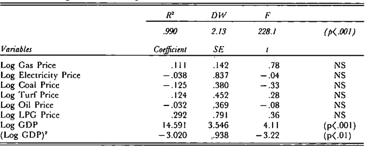
Table 3.6: Regression Results for LPG
Variables
R2 D 14/ F
.990 2.13 228.1
Coefficient SE t
( p<.Oo t )
Log Gas Price ,I 11 i142 ,78 NS
Log Electricity Price --.038 .837 --.04 NS Log Coal Price -.125 .380 -.33 NS Log Turf Price .I 24 .452 .28 NS Log Oil Price -.032 ,369 --.08 NS
Log LPG Price .292 .791 .36 NS
Log GDP 14.591 3.546 4.11 (p(.001)
(Log GDP)~ -3.020 ,.938 -3.22 (p(.01)
A summary of these analyses is given in Table 3.7 in relation to price and GDP coefficients. The three fuels ~- electricity, oil and LPG --showed significant departures from the doUble-log formulation as regards the relationship with GDP and hence have declining elasticities with respect to GDP. As already mentioned, the non-significant results shown for gas, coal and turf with respect to GDp cannot be taken immediately to mean no dependency on GDP, bec,ause t tests assume the other variables fitted. Thus a significant result for (log GDP)2 definitely means a departure from a linear relationship, but non-significant results for both log GDP and (log GDP)2 need not ruile out the linear effect being significant if entered alone.
[image:43.506.73.438.112.257.2]h is also true that the significance of a price effect is tested assuming all other prices fitted and since, as was remarked in Chapter 2, some prices are fairly highly correlated with oihers, there is some danger that Table 3.7: Individual Fuels -- Regression Equation Results
Fuel R.~ GDP GDW Pc, P~: Pc Pv ’Do P,.
Gas .984 NS NS ***i NS * NS NS **
Electricity .998 *** *** * * NS NS NS NS
Coal .834 NS NS * ~ NS * ** * NS
Turf .808 * NS NS’ NS NS NS NS NS
Oil .987 *** *** * NS NS NS * NS
LPG .990 *** *** NSI NS NS NS NS NS
* = Statistically significant at 5% ** -- Statistically significant at I% *** = Statistically significant at .1%
.MoI)rLS FOR INDIVIDUAL FURLS: TIME SERIES ANALYSES 33
true price effects are being obscured. Ideally, each model should be refined by dropping some price variables in accordance with prior knowledge rather than purely on the indications of this first stage of analysis. Had the analyses been conducted by sector, rather than
nationally, such objective refnement would probably have been more achievable. For example, in the domestic sector, oil is a central heating
fuel which electricity is only to a slight degree, so it would be plausible to leave each price out of the other’s equation. But oil and electricity could be competitors in the transport sector, for example, so that it is difficult to visua]ise the national picture.
The following procedure seems the best compromise between the danger of obscuring effects by leaving excessive variables in the equations and the
arbitrary ruling out of substitution possibilities implied by dropping price variables. Any significant price variable was retained in any equation, as was own price whether significant or not and any variable with a large, even if not quite significant, coefficient. In the case of turf, the coal price variable was included in spite of its low coefficient in Table 3.4, because
of the high cross-price coefficient in Table 3.3.
Returning now to the investigation of the possible addition of a lagged dependent variable to the fuel equations, it was seen that in only two of
the six equations would the variable have been statistically significant. For coal, this significance seems to be a phenomenon associated with the outlier nature of the 1975 quantity. That leaves the electricity equation, which had been well fitting as estimated by (3.6), but the lagged variable was none the less significant. Interpretation poses a problem. For the
reasons given earlier, it hardly seems a logical consequence of lagged price or GDP effects. Some type of partial adjustment mechanism may be conceivable, but electricity would not have seemed the likeliest fuel to exhibit this. However, the forecasting properties of the two possible electricity equations are almost identical, if the long-run coefficients are taken for the lagged equation. The coefficient of lagged electricity was .31 and the log GDP and (log GDP)2 coefficients were 4.780 and -.963 respectively. Dividing the latter by .69 (=1--.31) gives the long-run coefficients of 6.93 and - 1.39, nearly the same as in Table 3.2.
The details of the finally modified equations are given in Table 3.8. Note that the turf equation shows no significant coefficient and has a significantly low DW value and the lowest R2 has fallen greatly.
3.4 Elasticities
Table 3.8: A4odified Individual Fuel Equations
The Variables in the Equations
ODe G’I.)P~ PG Pl~ Pc PT Pc, PI.
Gas Yes No Ves No Yes No No Yes Electricity Yes Yes Yes Yes No Yes Yes No Coal Yes No Yes No Yes Yes Yes No Turf Yes No No No Yes Yes No No Oil Yes Yes Yes No No No Yes No LPG Yes Yes No No No No No Yes
t values R2 D I’V
Gas 2.5 NA -- 15.6 NA 2.2 NA NA 7.5 .98 1.5 Electricity 7.1 --5.1 -- 2.9 --2.8 NA ’ 2.6 2.7 NA .99 1.7 Coal 1.5 NA -- 4.6 NA --3.5 4.0 6.3 NA .82 1.5 Turf --0.6 NA NA NA -- .2 0.6 NA NA .30 0.5 Oil 5.9 -4.5 3.5 NA NA NA -4.1 NA .99 1.7 LPG 7.6 -6.3 NA NA NA ’ NA NA 1.6 .99 1.9
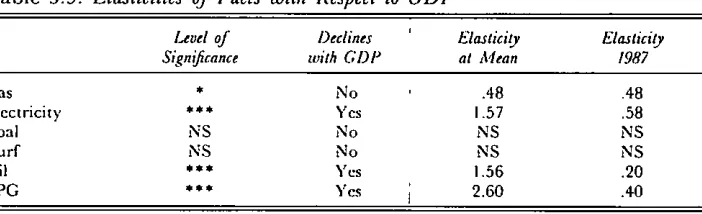
the GDP variable, or variables. Tile one exception is for turf, because poor though the unreduced equation was, the reduced one is even worse. Perhaps turf" was supply constrained at various times, or seriously affected by other variables not taken into account at all in this stud;,,. The GDP elasticities are shown in Table 3.9 and are given at mean values of GDP and, obviously more interestingly, at 1987 values. For gas, which had a significant relationship with GDP whcn the ’squared variable was dropped,
the elasticity is constant of course. So, for example, a 1 per cent increase in real GDP would currcntly lead to an increase of .6 per cent in electricity demand. The approximation inherent in using Equation (3.6),
which cannot be expected to hold indefinitely, makes it advisable to use
Table 3.9: Elasticities of Fuels with Respect to GDP
Level of Declines IzTastidty Elasticity
Significance with GDP at Mean 1987
Gas * No .48 .48
Electricity *** Yes 1.57 .58
Coal NS No NS NS
Turf NS No NS NS
Oil *** Yes 1.56 .20 LPG *** Yes 2.60 .40
* = Statistically significant at 5% *** = Statistically significant at .1°/~)