Continuous Observation Partially Observable Semi Markov Decision Processes for Machine Maintenance

Continuous-Observation Partially Observable Semi-Markov Decision

Processes for Machine Maintenance

Mimi Zhang, Matthew Revie

Partially observable semi-Markov decision processes (POS-MDPs) provide a rich framework for planning under both state transition uncertainty and observation uncertainty. In this paper, we widen the literature on POSMDP by studying discrete-state, discrete-action yet continuous-observation POSMDPs. We prove that the resultantα-vector set is continuous and therefore

propose a point-based value iteration algorithm. This paper also bridges the gap between POSMDP and machine maintenance by incorporating various types of maintenance actions, such as actions changing machine state, actions changing degradation rate, and the temporally extended action “do nothing”. Both finite and infinite planning horizons are reviewed, and the solution methodology for each type of planning horizon is given. We illustrate the maintenance decision process via a real industrial problem and demonstrate that the developed framework can be readily applied to solve relevant maintenance problems.

Index Terms—Condition-based maintenance, degenerate distri-bution, imperfect maintenance, multi-state systems, point-based value iteration.

ABBREVIATIONS& ACRONYMS

• SMDP: Semi-Markov Decision Process

• POMDP: Partially Observable Markov Decision Process

• POSMDP: Partially Observable Semi-Markov Decision

Process

• ECD: Expected Cumulative Discounted

• RGF: Rapid Gravity Filter

NOTATION

• S: State set

• A: Action set

• O: Continuous observation space

• Uz: Sojourn time between the zth and the (z+1)st

transitions

• Tz: Time of thezth transition:Tz=∑zk=−10Uk

• S¨z: Machine’s state at epoch z

• St: Machine’s state at timet:St=S¨z fortz≤t<tz+1

• A¨z: The maintenance action taken at epochz

• At: The maintenance action taken at timet: At=A¨z for

tz≤t<tz+1

• O¨z: The observation collected at epochz

• pi j(a): Transition probability: if the machine is in state

i and maintenance action a is taken on it, then it will

transfer to state j with probability pi j(a)

• Fi j(u;a): Sojourn time distribution function: if the

ma-chine is in state i and will transfer to state j under

maintenance action a, then the sojourn time follows

Fi j(u;a)

Mimi Zhang and Matthew Revie are with the Department of Management Science, University of Strathclyde, Glasgow, G1 1XW, UK

• fi j(u;a): Density function ofFi j(u;a)

• gi(o;a): Density function of the observation: if the

ma-chine is in state i and maintenance action a is taken on

it, then the observation has density functiongi(o;a)

• bbb¨z: Decision maker’s belief state at epoch z: ¨bbbz =

(b¨1_z,· · ·,b¨n_z)

• bbb¨t: Decision maker’s belief state at time t: ¨bbbt =bbb¨z for

tz≤t<tz+1

• R1(S¨z,A¨z): Immediate reward at epoch z

• R2(S¨z,A¨z): Reward with rate over the period(tz, tz+1) • R(bbbt,π(bbbt)): Instantaneous reward at timetfor the SMDP

model

• R₁(S¨z,A¨z): Immediate reward at epochzfor the POSMDP

model

• R₂(S¨z,A¨z): Reward with rate over the period(tz, tz+1)for the POSMDP model

• R(bbbt,π(bbbt)): Instantaneous reward at timet for the

POS-MDP model

• θ: discount factor

• w: Finite or infinite planning horizon

• π(·): Policy, mapping belief states into actions

• Vπ(·): Value function

• {α_zk}k:α-vector set at epochz

I. INTRODUCTION

The emergence of technologically advanced data-collecting techniques, such as vibration monitoring, acoustics and physical condition monitoring, have been explored for improving reliability prediction and maintenance decision making. One popular choice of incorporating condition monitoring information into traditional lifetime data is through the proportional hazard model [1], [2], [3]. Another common choice is to directly model conditioning monitoring data by a stochastic process, e.g., the gamma process, [4], [5], [6]; failure is defined as the process exceeding a (random) threshold. However, in many practical applications,

the physical condition of a machine1 is characterized by a discrete set of states; see, e.g., [7] for road maintenance, [8] for

power system management, [9] for production scheduling, and [10] for optimal replacement of wind turbines. Moreover, in many cases we are not permitted exact observations of the state of the machine. We can only model what is observable as probabilistically related to the true state of the machine; see, e.g., [11], [12], and [13]. In general, the partial observability stems from two sources. Firstly, different states can give the same observation. Secondly, sensor readings are noisy: observing the same state can result in different sensor readings.

For such applications, the decision-theoretic model of choice is a partially observable Markov decision process (POMDP). POMDPs provide a rich framework for planning under both state transition uncertainty and observation uncertainty. The POMDP model has been widely used for asset management under uncertainty; see [14] and the references therein. Note that POMDPs are not well suited for machine maintenance, as they are based on a discrete time step: the unitary action taken at

timet affects the state and reward at timet+1. Yet, in machine maintenance, many maintenance actions take nontrivial time.

For example, if we leave a machine operating for a period of time, then the action taken on the machine is “do nothing”, and the duration of “do nothing” is the time period over which the machine is operating. Hence, in the present paper, we introduce temporally extended actions into the POMDP model by studying the partially observable semi-Markov decision process (POSMDP). The POSMDP model was first proposed by [15] and then studied by, e.g., [16], [17] and [18].

Though the POSMDP model has existed for decades, there has been little effort in bridging the gap between POSMDP and machine maintenance. Moreover, the documented works on employing POSMDP in machine maintenance are all concerned with simple maintenance actions (e.g., perfect repair). A POSMDP problem is studied by [13] in which the state set contains only two elements, the maintenance action (repair) is simply perfect, and the observation space is discrete. In many practical problems, it is common for observations to be continuous, because sensors often provide continuous readings. Recently, [19], [20] and [21] coupled the POSMDP model with the Bayesian control chart. They assumed that, conditioned on the state of the machine, the observation vector follows a multivariate normal distribution. However, technically, the Bayesian control chart is introduced only to provide a threshold: if the posterior reliability of the machine drops to that threshold, a maintenance action will be performed. Moreover, the maintenance model they studied is rather simple: the state set only consists of two unobservable states and one observable failure state, and maintenance actions are assumed to be perfect. Another related work can be found in [22], who considered a POSMDP problem with continuous state space and continuous observation space. They then adopted a density projection method to convert the POSMDP problem into a semi-Markov decision process (SMDP) problem.

To date, the POSMDP model has not been developed for the case of discrete states, discrete actions and continuous observations. In addition, many of the applications of the POSMDP have failed to capture the subtleties of the maintenance actions available to decision makers. Other than perfect repair and minimal repair, maintenance engineers can often take an action which resets the machine to an earlier state but not to new, and/or reduces the rate of future degradation. An example of the former would be replacing some components of a complex machine and, for the latter, replacing the oil in an automobile to slow down deterioration of the gearbox. Motivated by the practical need of a maintenance-optimization tool for partially observable deteriorating systems, the current work proposes a POSMDP model with discrete state, discrete action yet continuous observation. The developed framework is generic and can be applied to a variety of cases: finite planning horizon, infinite planning horizon, and multi-dimensional observation space.

The remainder of the paper is organized as follows. In Section II, we derive the finite- and infinite-planning-horizon value functions of the continuous-observation POSMDP. In Section III, we study some properties of the value functions and develop a value-iteration algorithm. In Section IV, we illustrate, via an industrial problem, the incorporation of different maintenance actions (perfect, imperfect or minimal) into the POSMDP model. Section V gives numerical studies to show the feasibility and effectiveness of the proposed methods. Section VI concludes the paper.

II. MODELFORMULATION

We begin with a brief review of the SMDP model and then generalize the SMDP model to the POSMDP model with the observation space being continuous. The reader is referred to [23] for the SMDP model, and [24] for partially observable Markov processes.

1_{A machine in this context could be any piece of mechanical equipment which requires periodic maintenance due to deterioration of its internal components}

A. Semi-Markov Decision Process

The standard SMDP model consists of two finite sets:

• a finite set ofn states, labelled byS={1,2,· · ·,n}; • a finite set ofvactions, labelled byA={1,2,· · ·,v}.

Here, both n andv are positive integers. The states of the SMDP model are indeed the states of the machine, and a higher

state represents a higher deterioration level of the machine. Typically, state 1 represents an excellent condition of the machine,

while state n represents failure. The action set is composed of all the available maintenance actions that can be taken on the

machine, e.g., A={1=“do nothing”,2=“imperfect repair”,· · ·,v=“replace”}.

The state of the machine is unveiled (e.g., by thorough inspection) at random time points. Let{_S¨_{z, z∈Z}denote the evolving}

process of the state, with ¨Sz taking values from the state set S. Here, Z is the set of nonnegative integers. Let {A¨z, z∈Z}

denote the action process to control the deterioration of the machine. At epoch z(∈Z), after knowing the state (i.e., the value

of ¨Sz), a decision maker chooses an action ¨Az=a from the action set A, making the state of the machine change at the next

epoch (z+1). The sojourn time between the zth and the (z+1)st epochs is a positive random variable, denoted byUz. Let

Tz denote the time of the zth transition: Tz=∑_k=z−1₀Uk; that is, Tz is the time at which the state of the machine transits from

¨

Sz−1 to ¨Sz. Lettz (resp.uz) denote, from the generic point of view, the value ofTz (resp.Uz). Let St denote the state of the

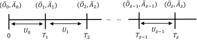
machine at timet (≥0) andAt denote the action taken at timet. Clearly, fortz≤t<tz+1, we haveSt=S¨z andAt=A¨z. Figure

1 illustrates the maintenance decision process under the SMDP setting.

𝑇

_𝑧−1

𝑇

1

𝑇

2

𝑇

𝑧

𝑈

₁

𝑈

_𝑧−1

𝑈

₀

0

… …

(𝑆̈

1

, 𝐴̈

1

)

)

(𝑆̈

_𝑧−1

, 𝐴̈

_𝑧−1

)

(𝑆̈

2

, 𝐴̈

2

)

)

(𝑆̈

0

, 𝐴̈

0

)

)

(𝑆̈

𝑧

, 𝐴̈

𝑧

)

[image:3.612.142.470.285.353.2]

At epoch 𝑧, we observe the state 𝑆̈𝑧. According to the state, we take action 𝐴̈𝑧. The machine remains at the present state for 𝑈𝑧 units of time and then moves to state 𝑆̈𝑧+1 at time 𝑇𝑧+1.

Fig. 1: At epoch z, we observe the state ¨Sz. According to the state, we take action ¨Az. The machine remains at the present

state forUz units of time and then moves to state ¨Sz+1at timeTz+1.

The process {(S_t,At), t≥0}is called an SMDP, if the following two Markovian properties are satisfied.

• Given the present state, states in the future do not depend on the states in the past.

• Given the present state and the next state, the distribution of the sojourn time does not depend on the states in the past.

The above two Markovian properties can be mathematically formulated as follows. Write pi j(a) (i∈S,a∈Aand j∈S) for

the law of motion of the SMDP at epoch z:

pi j(a) =Pr(S¨z+1=j|S0¨ ,A0¨ ,U0,· · ·,S¨z=i,A¨z=a).

Then we have

pi j(a) =Pr(S¨z+1=j|S0¨ ,A0¨ ,U0,· · ·,S¨z=i,A¨z=a) =Pr(S¨z+1=j|S¨z=i,A¨z=a).

Conditioned on the event that the next state is j,Uz has the distribution functionFi j(u; a):

Fi j(u; a) =Pr(Uz≤u|S0¨ ,A0¨ ,U0,· · ·,S¨z=i,A¨z=a,S¨z+1=j) =Pr(Uz≤u|S¨z=i,A¨z=a,S¨z+1=j),

withu>0 andFi j(0; a) =0. For example, if the maintenance action taken at epoch zis “repair”, then Fi j(u; a) models the

duration of the repair; if the maintenance action taken at epochzis “do nothing”, thenFi j(u; a)models the time length of the

machine staying in statei. Let fi j(u; a)denote the density function ofUz. By the law of total probability, we have

Pr(Uz≤u,S¨z+1=j|S¨z=i,A¨z=a) =Fi j(u; a)pi j(a).

That is, given that the current state is i and actiona is taken on the machine, the state of the machine will, with probability

Fi j(u; a)pi j(a), change to jwithin uunits of time.

Remark 1. A decision rule πz at epoch z is a vector consisting of probabilities that are assigned to available actions.

Specifically, an elementπz(a)ofπz is the conditional probability of choosing action a∈Aat the zth epoch: πz(a) =Pr(A¨z=

a|_S0¨ _,A0¨ _{,U0,· · ·,S}¨

z=i). When concerned with finite (resp. infinite) horizon SMDPs, a policy π is a finite (resp. infinite)

sequence of decision rules π ={π0,π1,π2,· · · }. π is called a Markov policy if πz(a) depends only on the present state:

πz(a) =Pr(A¨z=a|S¨z=i).

Naturally, machine maintenance will bring about monetary costs and rewards. For the current work, we might treat a cost as

a negative reward. At epochz, after knowing the state ¨Sz, the decision maker chooses an action ¨Az. Resulted from the action ¨Az

is shut down for maintenance, the immediate reward could be the cost of buying a new gearbox; the loss of the electricity

income per day could be the reward rate. Let R(St,At)denote the instantaneous reward function of the SMDP model:

R(St,At) =

R1(S¨z,A¨z), ift=tz;

R2(S¨z,A¨z), iftz<t<tz+1.

B. Partially Observable semi-Markov Decision Process

Extending the SMDP setting, the POSMDP model further deals with uncertainty resulting from imperfect observations. It allows for maintenance scheduling for machines that are only partially observable to the decision maker. More formally, let

{_O¨_{z, z∈Z} denote the information process, with ¨Oz taking values from a continuous observation spaceO. The observation}

space O can be multi-dimensional. For example, an array of sensors (such as sonars, laser-range finders, video cameras and

microphones) are equipped to provide partial information. Define a density function gi(o;a), modelling the probability of the

event{O¨z=o} given that the action taken at epoch(z−1)isa and that the current physical state of the machine isi:

Pr(O¨z∈O|A¨z−1=a,S¨z=i) = Z

O

gi(o;a)do, (1)

where _O is a subset of O. Here and in the following, the symbol “d” denotes an infinitesimal change in a quantity. An

assumption employed here is that the distribution of ¨Oz depends only on the last action and the present sate.

Now the maintenance decision process proceeds as follows. At epoch z, the decision maker receives an observation ¨Oz.

According to the received information, the decision maker updates his belief regarding the current state ¨Sz. According to the

newly updated belief, the decision maker then chooses an optimal action to control or detect the deterioration of the machine,

believing that the machine will remain at the present state for Uz units of time and then move to state ¨Sz+1 at time Tz+1.

At epoch (z+1), the decision maker collects a new observation ¨Oz+1, and the whole maintenance decision process repeats.

Note that, for the SMDP model, the present state ¨Sz is exactly known, and the decision maker chooses an action based on the

present state. However, for the POSMDP model, the decision maker can only form a subjective judgement on the state of the

machine and chooses an action based on such judgement. The underlying true state at epoch (z+1), i.e. ¨Sz+1, need not be

different from ¨Sz.

The decision maker’s judgement on the state of the machine can be represented by a vector of probabilities (called belief state): ¨bbbz= (b¨1z,· · ·,b¨nz), where ¨biz (1≤i≤n) is the decision maker’s probability with which the condition of the machine at

epochz is in statei: ¨bi_z=Pr(S¨z=i|·).The conditional term to the right of the vertical slash will be detailed in Equation (2).

We have ¨bi_z≥0 and∑ni=1b¨iz=1. At time 0, the decision maker’s belief state ¨bbb0 characterizes the prior knowledge regarding

the condition of the machine before the beginning of the sequential decision making. Let bbbt denote the decision maker’s

belief state at time t: bbbt =bbb¨z for tz≤t <tz+1. It is easy to prove that the whole information available by epoch z, i.e. {bbb0¨ ,A0¨ ,U0,· · ·,O¨z−1,A¨z−1,Uz−1,O¨z}, can be summarized by ¨bbbz, and to calculate ¨bbbz+1, it is sufficient to know ¨bbbz (see, e.g.,

[25]). Therefore, we can incorporate the information received over the period (Tz,Tz+1], i.e.,{A¨z,Uz,O¨z+1}, and the previous

belief state ¨bbbz to calculate the posterior distribution of the state of the machine. This is accomplished by applying the Bayes

theorem:

¨

bi_z+1=Pr(S¨z+1=i|bbb¨z,A¨z=a,Uz=u,O¨z+1=o) =

Pr(Uz=u,O¨z+1=o,S¨z+1=i|bbb¨z,A¨z=a)

Pr(U_z=u,O¨z+1=o|bbb¨z,A¨z=a)

, (2)

in which we have

Pr(U_z=u,O¨z+1=o,S¨z+1=i|bbb¨z,A¨z=a)

=Pr(Uz=u,O¨z+1=o|bbb¨z,A¨z=a,S¨z+1=i)Pr(S¨z+1=i|bbb¨z,A¨z=a)

=

n

∑

j=1

¨

b_zjPr(Uz=u,O¨z+1=o|S¨z=j,A¨z=a,S¨z+1=i)Pr(S¨z+1=i|S¨z=j,A¨z=a)

=

n

∑

j=1

¨

b_zjfji(u;a)gi(o;a)pji(a), (3)

and

Pr(Uz=u,O¨z+1=o|bbb¨z,A¨z=a) = n

∑

i=1

Pr(Uz=u,O¨z+1=o,S¨z+1=i|bbb¨z,A¨z=a)

=

n

∑

i=1

n

∑

j=1

¨

b_zjfji(u;a)gi(o;a)pji(a). (4)

In Equation (3), we have utilized the fact that the two conditional events,{Uz=u|S¨z=j,A¨z=a,S¨z+1=i}and{O¨z+1=o|A¨z=

conditioned on executing ¨Az=a and, afteruunits of time, observing ¨Oz+1=o; that is, ¨bbbz+1=llla(bbb¨z,u,o). Figure 2 illustrates

the maintenance decision process under the POSMDP setting.

𝑇

_𝑧−1

𝑇

₁

𝑇

2

𝑇

𝑧

𝑈

1

𝑈

𝑧−1

𝑈

₀

0

… …

(𝑂̈

₁

, 𝐴̈

₁

)

)

(𝑂̈

_𝑧−1

, 𝐴̈

_𝑧−1

)

(𝑂̈

2

, 𝐴̈

2

)

)

(𝑂̈

₀

, 𝐴̈

₀

)

)

(𝑂̈

_𝑧

, 𝐴̈

_𝑧

)

[image:5.612.143.473.92.160.2]

At epoch 𝑧, we receive an observation 𝑂̈𝑧= 𝑜. According to the value of (𝒃̈𝑧−1, 𝐴̈𝑧−1, 𝑈𝑧−1, 𝑂̈𝑧), we update the belief state to 𝒃̈𝑧 and take action 𝐴̈𝑧= 𝜋(𝒃̈𝑧). The machine remains at the present state for 𝑈𝑧 units of time and then moves to state 𝑆̈𝑧+1 at time 𝑇𝑧+1.

Fig. 2: At epochz, we receive an observation ¨Oz. According to the value of(bbb¨z−1, ¨Az−1,Uz−1, ¨Oz), we update the belief state

to ¨bbbz and take action ¨Az. We will collect a new observation ¨Oz+1at time Tz+1, the time point at which we think the state of the machine will change to ¨Sz+1.

The belief state ¨bbbz is a probability mass function over S. All belief states are contained in an (n−1)-dimensional simplex

∆, implying that we can represent a belief state using (n−1) numbers. For the SMDP model, a policy is a mapping from

states to actions (see Remark 1). However, for the POSMDP model, due to the partial observability, a policyπ is a mapping

from belief states to actions. Hence, we might re-write the policyπ into a functional formπ(·):∆→A. In other words, given

the belief state ¨bbbz, the policy π will indicate which action to take at epoch z: ¨Az=π(bbb¨z). If π(bbb¨z) =a (∈A), then, with

probability ¨bi_z (1≤i≤n), the decision maker can earn an immediate rewardR1(i,a)and a reward with rateR2(i,a)over the

period (tz, tz+1). Hence, the instantaneous reward function for the POSMDP model is given by

R(bbbt,π(bbbt)) =

_R

1(bbb¨z,π(bbb¨z)), ift=tz, R2(bbb¨z,π(bbb¨z)), iftz<t<tz+1, in which

R1(bbb¨z,π(bbb¨z)) = n

∑

i=1

¨

bi_zR1(i,π(bbb¨z)), and R2(bbb¨z,π(bbb¨z)) = n

∑

i=1

¨

bi_zR2(i,π(bbb¨z)).

Apparently, each policy will induce an expected cumulative (and possibly discounted by a discount factor) reward. The objective of a POSMDP problem is to work out a policy that will maximize the expected cumulative reward, which is the topic of Section II-C.

Now we can briefly define the POSMDP model which can be specified by a tuple hS, A, O, pi j(a), Fi j(u;a), gi(o;a),

R(bbbt,π(bbbt)),θ,wi, whereθ (∈(0,1))is a discount factor, andw(>0)is a planning horizon. The discount factor, analogous

to the interest rate, is for calculating the present value of future earnings. The planning horizon can be finite or infinite.

Remark 2. Note that the parameters in pi j(a), Fi j(u;a) and gi(o;a) have to be estimated from the observations of

{O¨1,O¨2,O¨3,· · · }. This is a common parameter-estimation problem in the area of hidden Markov model. Efficient methods are available, e.g., the Baum-Welch algorithm proposed by [26]. We do not discuss parameter estimation here, as it is outside the scope of this paper.

C. Value Function

For a POSMDP problem, the decision maker’s objective is to work out a maintenance policy that optimizes a given reward criterion. Two criteria have been extensively used in the literature: the expected cumulative discounted (ECD) reward and the long-run average expected reward; see, e.g., [27]. For the current work, we only concentrate on the ECD reward. The ECD reward is easier to analyze and understand than the long-run average expected reward, since discounting lands itself naturally to economic problems in which future earnings are discounted by the interest rate. Moreover, the ECD reward criterion can be interpreted as putting more weight on initial decisions.

The quality of a policy, π, can be assessed by a value function Vπ(·):∆→R, where R is the set of real numbers. The

function valueVπ(bbb) of the policyπ is the ECD reward that will be earned over the planning horizon[0,w]when starting in

belief statebbb∈∆. Among all candidate policies, if π yields the maximal function valueVπ(bbb) for allbbb∈∆, then π is called the optimal policy; the optimal policy specifies the optimal action to execute at the current epoch, assuming that the decision

maker will also act optimally in the future. In what follows, we let π∗ denote the optimal policy.

At timetz (<w), given that the decision maker’s belief state has been updated to ¨bbbz, we then need to determine the optimal

maintenance action ¨Az. LetVz(bbb¨z)denote the ECD reward (discounted to timetz) the decision maker can obtain by following

the optimal policyπ∗:

Vz(bbb¨z) =E Z w

tz

exp(−θ(t−tz))R(bbbt,π∗(bbbt))dt

¨ bbbz

,

When the planning horizon is finite, i.e.,w<∞, define ¯w=max{k:tk≤w}. The ECD reward can be further written into

Vz(bbb¨z) =E

R1(bbb¨z,π∗(bbb¨z)) +

1−exp(−θUz)

θ R2(

¨

bbbz,π∗(bbb¨z))

¨ bbbz

+E " ¯ w−1

∑

k=z+1 exp(−θ k−1

∑

r=z

Ur)

R1(bbb¨k,π∗(bbb¨k)) +

1−exp(−θUk)

θ R2(

¨ b

bbk,π∗(bbb¨k))

¨ bbbz

# +E " exp(−θ ¯ w−1

∑

r=z

Ur)

R1(bbb¨w¯,π∗(bbb¨w¯)) +

1−exp(−θ(w−Tw¯))

θ R2(

¨

bbbw¯,π∗(bbb¨w¯))

¨ b bbz

#

.

If π∗(bbb¨z) =a(∈A), we have

Eexp(−θUz) bbb¨z

=

Z w−tz

0

exp(−θu)Pr(Uz=u|bbb¨z,A¨z=a)du

=

Z w−tz

0

n

∑

i=1

¨ bi_z

n

∑

j=1

exp(−θu)Pr(S¨z+1=j,Uz=u|S¨z=i,A¨z=a)du

=

Z w−tz

0

n

∑

i=1

¨ bi_z

n

∑

j=1

exp(−θu)fi j(u; a)pi j(a)du.

Define an n-dimensional vector ¯Ra_z with elements

¯

Ra_z(i) =R1(i,a) + 1

θ

1−E

exp(−θUz)

bbb¨_z R₂(i,a), 1≤i≤n.

Then the ECD reward can be written in a recursive form:

Vz(bbb¨z) =max

a∈A

   n

∑

i=1 ¯ Ra_z(i)b¨i_z+

w−tz

Z

0

Z

O

Pr(Uz=u,O¨z+1=o|bbb¨z,A¨z=a)exp(−θu)Vz+1(llla(bbb¨z,u,o))dodu 





. (5)

Here, Vz+1(llla(bbb¨z,u,o)) is the ECD reward (discounted to time tz+1) when starting in belief state ¨bbbz+1=llla(bbb¨z,u,o). The

expression for the probability Pr(Uz=u,O¨z+1=o|bbb¨z,A¨z=a)is given by Equation (4). When the planning horizon is infinite,

i.e., w= +∞, we have

Vz(bbb¨z) =E

R1(bbb¨z,π∗(bbb¨z)) +

1−exp(−θUz)

θ R2(

¨ b b

bz,π∗(bbb¨z))

¨ bbbz

+E " ₊ ∞

∑

k=z+1 exp(−θ k−1

∑

r=z

Ur)

R1(bbb¨k,π∗(bbb¨k)) +

1−exp(−θUk)

θ R2(

¨ b b

bk,π∗(bbb¨k)) ¨ b bbz

#

=max

a∈A

   n

∑

i=1 ¯ Ra_z(i)b¨i_z+

∞ Z

0

Z

O

Pr(Uz=u,O¨z+1=o|bbb¨z,A¨z=a)exp(−θu)Vz+1(llla(bbb¨z,u,o))dodu 





. (6)

The optimal action to take at epochzshould be the one that maximizesVz(bbb¨z):

π∗(bbb¨z) =arg max

a∈AVz(

¨ bbbz).

From Equation (5) we know thatVz is a function ofVz+1. We might simply write the recursion (5) asVz=HVz+1:

(HVz+1)(bbb¨z) =max

a∈A

   n

∑

i=1 ¯ Ra_z(i)b¨i_z+

w−tz

Z

0

Z

O

Pr(Uz=u,O¨z+1=o|bbb¨z,A¨z=a)exp(−θu)Vz+1(llla(bbb¨z,u,o))dodu 





. (7)

H is called the Bellman backup operator [28]. This notation is defined here only to facilitate the proof for Proposition 2. Note

that, if the planning horizon wis finite, the value functionVz+1(·)changes with the value ofUz. Yet, if the planning horizon

is infinite, the value functionVz+1(·)does not change with uz. As will be proved in Proposition 2, bothVz(·) andVz+1(·)are

identical to the underlying true value function, denoted byV(·). The main objective of Section III is to approximate this true

value function. Whenw= +∞, the recursion (6) can be written in the Bellman functional formV =HV:

(HV)(bbb¨z) =max

a∈A

   n

∑

i=1 ¯ Ra_z(i)b¨i_z+

∞ Z

0

Z

O

Pr(Uz=u,O¨z+1=o|bbb¨z,A¨z=a)exp(−θu)V(llla(bbb¨z,u,o))dodu 





III. A VALUE-ITERATIONALGORITHM

In the literature, there are several algorithms for computing an optimal policy: value iteration, policy iteration and linear programming; see, e.g., [27]. Herein, we develop a value-iteration algorithm. Value-iteration algorithms compute a sequence of value functions in a backward manner starting from a lower bound on the true value function. We first concentrate on the theoretical basis on which to develop the value-iteration algorithm.

Proposition 1. Let<·,·>denote the inner product operator. The optimal value function Vz(·)at time tz can be expressed as

Vz(bbb) = sup

{αzk}k

<αzk, bbb>, bbb∈∆.

Here, {α_zk}k is a continuous set of vectors, andα_zk= (α_zk(1),· · ·,α_zk(n)).

Proof. We here only prove thatVz(·)can be written into the inner-product form, assuming that{α_zk}k is a continuous set for

z<w. The continuity of the set¯ {α_zk}k is proved in Appendix A.

The proof is done via induction. At epoch ¯wwe have

Vw¯(bbb¨w¯) =R1(bbb¨w¯,π∗(bbb¨w¯)) + 1

θ

1−Eexp(−θ(w−Tw¯))

bbb¨w¯ R2(bbb¨w¯,π∗(bbb¨w¯)) =max

a∈A<R¯

a

¯

w, bbb¨w¯> .

Then we define the set {α_wk_¯}k={R¯aw¯}a∈A and haveVw¯(bbb¨w¯) =max {αkw¯}k

<α_wk_¯, bbb¨w¯>.

Now assume thatVz+1(llla(bbb¨z,u,o))can be written into the inner-product form:

Vz+1(llla(bbb¨z,u,o)) = sup

{α_z+k ₁}k

<α_z+k ₁, llla(bbb¨z,u,o)> .

From Equation (2) we have

Vz+1(llla(bbb¨z,u,o)) = sup

{α_z+k ₁}k n

∑

i=1

α_z+k ₁(i)li_a(bbb¨z,u,o) =

sup {α_z+k ₁}k

∑ni=1αz+k 1(i)∑

n

j=1b¨

j

zfji(u;a)gi(o;a)pji(a)

Pr(Uz=u,O¨z+1=o|bbb¨z,A¨z=a)

.

SubstituteVz+1(llla(bbb¨z,u,o))into Equation (5):

Vz(bbb¨z) =max

a∈A







<R¯a_z,bbb¨z>+

w−tz

Z

0

Z

O

exp(−θu) sup

{α_z+k ₁}k

( n

∑

i=1

α_z+k ₁(i)

n

∑

j=1

¨

b_zjfji(u;a)gi(o;a)pji(a) ) dodu    =max

a∈A





 <_R¯a

z,bbb¨z>+

w−tz

Z

0

Z

O

exp(−θu) sup

{α_z+k ₁}k

( _n

∑

j=1 " _n

∑

i=1

α_z+k ₁(i)fji(u;a)gi(o;a)pji(a) #

¨ b_zj

) dodu    . (9)

Let δ_ka(u,o) = (δ_ka₁(u,o),· · ·,δ_kna(u,o))denote a vector-valued function:

δ_{k j}a(u,o) =

n

∑

i=1

αz+k 1(i)fji(u;a)gi(o;a)pji(a), 1≤j≤n. (10)

Note that, for fixed u ando, the cardinality of {δ_ka(u,o)} is exactly the cardinality of{α_z+k ₁}, andδ_ka(u,o)is independent of

¨ b b

bz. Then we have

Vz(bbb¨z) =max

a∈A

(

<R¯a_z,bbb¨z>+ Z w−tz

0

Z

Oexp(−θu){δ_kasup(u,o)}_k

<δ_ka(u,o), bbb¨z>dodu )

.

We can write

Vz(bbb¨z) =max

a∈A<R¯

a

z+

Z w−tz

0

Z

Oexp(−θu)arg{δ_kasup(u,o)}_k

<δ_ka(u,o), bbb¨z>dodu, bbb¨z>

=max

a∈A<δa(

¨ b b

bz), bbb¨z>,

where

δa(bbb¨z) =R¯az+ Z w−tz

0

Z

Oexp(−θu)arg{δ_kasup(u,o)}k

Then we can simply define the set {α_zk}k as

{α_zk}k= [

b b

b∈∆

{arg max {δa(bbb)}a∈A

<δa(bbb), bbb>}.

Therefore,{α_zk}kis a continuous set of vectors parameterized in the action set; that is, each vector is associated with an action,

which is the optimal action for the belief state that has such vector as the maximizing one. Consequently,Vz(bbb)can be put in

the desired form

Vz(bbb) = sup

{αzk}k

<αzk, bbb> .

The elements in {α_zk}k are usually called α-vectors. Let Ωz denote the set of α-vectors:Ωz={αzk}k. Using Proposition 1

we can readily prove that the value functionVz(bbb)is convex. Since the inner product operator is linear in its two arguments,

the convex property is given by the fact thatVz(bbb)is defined as the supreme of a set of convex (linear) functions.

Proposition 2. Let || · ||denote the supreme norm. For the Bellman backup operator H given by Equation (8) and two value functions Vz+1and Uz+1, it holds that||Uz−Vz||=||HUz+1−HVz+1||<||Uz+1−Vz+1||. Moreover, if Vz+1≥Uz+1, then Vz≥Uz.

That is, the backup operator H is a contractive and isotonic mapping.

The proof is given in Appendix B. According to Proposition 1, the space of value functions is closed under addition and scalar scaling. The contraction property further ensures that this space is complete. Therefore, the space of value functions together with the supreme norm form a Banach space. The Banach fixed-point theorem ensures the existence of a single fixed point and that the value iteration always converges to this point. The isotonic property ensures that value iteration converges monotonically.

Propositions 1 and 2 indicate that value iteration is a promising method for policy optimization. Equations (10) and (11)

provide a constructive way to define the set of vectors {αzk}k. The computation of theα-vector for a given belief pointbbb is

called a backup:

backup(bbb) =arg sup {αzk}k

<α_zk, bbb>=arg max {δa(bbb)}a∈A

<δa(bbb), bbb> .

Using the backup operator, the value ofVz(bbb)is simplyVz(bb) =b <backup(bbb),bbb>. A backup for the whole belief space requires

the computation of all theα-vectors. However, a whole backup is impossible when the observation space is continuous, because

the set {α_zk}k is continuous, having infinitely many vectors. Consequently, we employ the idea of point-based value iteration

(PBVI), which performs backup on a finite set of belief points [29]. Theα-vectors for the restricted set of belief points form

an approximation to the set {αzk}k, and they can be used to approximate the true value function for any belief point. Many

extensions have been suggested to the idea of PBVI. [30] provided a comprehensive overview of existing point-based solvers. In this paper we employ, with some modifications, the Perseus algorithm developed by [31].

An intuitive approach to selecting belief points would be to maintain a regular grid of belief points. One downside of such an approach is that it is highly probable that many of these belief points are not reachable. The Perseus algorithm starts with

collecting a setBof reachable belief points by using Algorithm 1, in which the initial belief pointbbbis provided by the decision

maker. Then the Perseus algorithm proceeds to value-function updating, performed only on the belief points in B. Particularly,

Algorithm 1 Random exploration

1: B={bbb}.

2: whilethe cardinality ofB is smaller than a thresholddo

3: Randomly simulate a state, denoted by j, according to the distributionbbb.

4: Uniformly simulate an action from A, denoted by a.

5: Randomly simulate a state, denoted by i, according to(pj1(a),pj2(a),· · ·,pjn(a)).

6: Randomly simulate a sojourn time, denoted by u, from the distribution fji(u;a).

7: Randomly simulate an observation, denoted byo, from the distribution gi(o;a).

8: Calculate the posterior distributionllla(bbb,u,o)according to Equation (2).

9: Addllla(bbb,u,o)toBand initializebbb tollla(bbb,u,o).

10: end while

given a setΩz+1of finiteα-vectors obtained at epochz+1, [31] developed Algorithm 2 for approximating the value function

Vz(·). Starting from epoch ¯w, repeatedly applying Algorithm 2 until we arrive atz=0 (forw<+∞) or until the value function

is stable (for w= +∞). Note that, for finite planning horizon, if the observation space is discrete (namely, the α-vector sets

are all discrete), then we need not use Algorithm 2; we can exactly derive every element in eachα-vector set. However, since

theα-vector sets for a continuous-observation POSMDP are all continuous (except the starting one), when employing the idea

Algorithm 2 Value-function updating

1: SetΩz to be empty and initialize ˜BtoB.

2: whileB˜is not empty do

3: Randomly sample a belief pointbbb from ˜B and computeα=backup(bbb)based on theα-vectors in the set Ωz+1.

4: if <α, bbb>is larger thanVz+1(bbb)then

5: Addα to the setΩz. Remove from ˜Ball the belief points that can be improved byα.

6: else

7: Add ˆα=arg max

{αk_z+1}k

<α_z+k ₁, bbb>to the setΩz. Remove from ˜Ball the belief points that can be maximized by ˆα.

8: end if 9: end while

Whenw is infinite, the Perseus algorithm requires that the value functionVz(·)be a lower bound onV(·). To this end, we

only need to makeVw¯(·)be a lower bound. We defineR= min

s∈S,a∈A{R2(s,a)} and set{α

k

¯

w}k={α}:

α(i) =

Z ∞

0

exp(−θu)Rdu=R

θ, i=1,· · ·,n.

α(i)is equivalent to the present value of the cash flow in which we only receive the minimal possible reward rate (no immediate

reward).

There are a number of potential disadvantages to Perseus though; see [30]. One is that the random exploration is not optimal in that it may not encounter most of the same points as the optimal policy. We therefore propose to start with a relatively

small size of B, e.g., 500 belief points. When the whole value-function updating procedure is completed, we add intoBnew

belief points by utilizing the newly computed optimal policy (see Algorithm 3). We iteratively apply Algorithms 2 and 3 until

Algorithm 3 Expand B

1: Initialize ¨B toB 2: foreachbbb∈B do

3: Randomly simulate a state, denoted by j, according to the distributionbbb.

4: Using the newly computed optimal policy to derive the optimal action forbbb: the action associated with the vector that

maximizesbbb.

5: Randomly simulate a state, denoted by i, according to(pj1(a),pj2(a),· · ·,pjn(a)).

6: Randomly simulate a sojourn time, denoted by u, from the distribution fji(u;a).

7: Randomly simulate an observation, denoted byo, from the distribution gi(o;a).

8: Calculate the posterior distributionllla(bbb,u,o)according to Equation (2)

9: Ifllla(bbb,u,o)6∈B, add¨ llla(bbb,u,o)to ¨B

10: end for 11: Return ¨B

the cardinality of B is larger than a pre-determined threshold.

IV. INCORPORATINGDIFFERENTMAINTENANCEACTIONS

The generic POSMDP model in Section II-B implies that maintenance actions (either changing machine state or changing deteriorating rate) can be fully characterized by the state transition matrices and sojourn time distributions. Perhaps a better way to explain how to characterize maintenance efficiency is through a heuristic example. In Section IV-A, we introduce a real industrial problem that involves different types of maintenance actions. In Section IV-B, we derive the corresponding state transition matrices to characterize the involved maintenance actions. In Appendix C, we present a detailed procedure of the belief point backup for the following industrial problem.

A. An Industrial Problem

To provide water service, a water utility operates water treatment works spreading over the UK. Raw water enters into a water treatment works, and clean water exits from the water treatment works. A water treatment works is a complex system with different components. Rapid gravity filters (RGFs) have been identified as the key components for purifying water. RGFs purify water by filtering water through a particular media. Experts within the water utility classify the condition of an RGF

(according to the condition of the media) into four different states:{“good”, “acceptable”, “poor”, “awful”}. The condition of

To guarantee that high water quality is achieved, the water utility records information on many features. An important feature is the turbidity in the water. Turbidity is the haziness of a fluid caused by individual particles and hence is naturally treated as a continuous random variable. The level of turbidity is recorded at key stages of the water treatment process (e.g., upon entry, pre-post processing at RGFs, on exit). When the ratio of outgoing to incoming water turbidity is close to zero, then the RGF is likely to be in a good condition. On the other hand, when the ratio is close to one, then the RGF is likely to be in a poor or even awful condition. Therefore, by comparing the turbidity in the water entering and exiting an RGF, we can infer from the probabilistic point of view the condition of the RGF.

To achieve better reliability and availability of the RGFs, experts in the water utility take maintenance actions on the RGFs. Typical maintenance actions are “do nothing”, “backwash”, “dose chemicals” and “replace”. Chemical dosing is to change the state of the RGF, while backwash will slow down the deterioration of the RGF. By replacing the media, the RGF will be renewed to the good state. Experts in the water utility backwash an RGF regularly, e.g., every other day, irrespective of the condition of the RGF, which is obviously not economical. If an RGF fails, the maintenance work will not be conducted until related funding is approved. During the downtime of the failed RGF, other RGFs in the water treatment works will bear the extra working load, leading to increased deterioration of the other RGFs or additional operational costs. Evidently, the current maintenance practice in the water utility is not efficient, and there is an economic need to better plan maintenance activities.

B. Characterizing Different Maintenance Actions

The state set of the RGF has four elements:S={1=“good”, 2=“acceptable”, 3=“poor”, 4=“awful”}. The action set is defined

as A={1=“do nothing”, 2=“backwash”, 3=“dose chemicals”, 4=“replace”}. Apparently, action 1 is minimal; actions 2 and 3 are imperfect; action 4 is perfect. We now discuss how to determine the state transition matrix for each action.

The state transition matrix of action 1 depends on the duration of action 1. For example, the transition probability p12(a=1)

when action 1 lasts for one day will be different from p12(a=1)when action 1 lasts for one month. In order to determine

the state transition matrix we have to first determine the duration of action 1, which is explained as follows. If the RGF is not maintained (or, equivalently, if the action taken is always “do nothing”), then the RGF will deteriorate gradually from state

i to statei+1 for i=1,2,3. Let random variable T_i1 denote the time length of the RGF staying in statei. For example, the

RGF will stay in state 1 forT₁1 units of time and then move to state 2. In practice, action 1 will be taken if the RGF is in the

good state, and will last until the RGF is in the acceptable state. Hence, we let the duration of action 1 be fixed at u∗₁ such

that the probability Pr(T1

1 <u ∗

1,T11+T21≥u ∗

1) is maximized. In other words, if the RGF is in state 1 and we do nothing for

u∗₁units of time, then by the end of action 1, the RGF will be in state 2 with the maximal probability. Consequently, the state

transition matrix can be derived:

P(a=1)

=



      

Pr(T1

1 ≥u ∗

1) Pr(T11<u ∗

1,T11+T21≥u ∗ 1) Pr(

2

∑

i=1

T_i1<u∗₁,∑3

i=1

T_i1≥u∗₁) 1−∑3

i=1

p1i(a=1)

0 Pr(T₂1≥u∗₁) Pr(T₂1<u∗₁,T₂1+T₃1≥u∗₁) 1−∑3

i=1

p2i(a=1)

0 0 Pr(T₃1≥u∗₁) Pr(T₃1<u∗₁)

0 0 0 1



       .

Before determining the state transition matrix for action 2, we need to modify action 2, the reason for which is explained as

follows. At epochz, after updating the belief state, the decision maker decides to backwash the RGF. The duration of backwash

is constant (not a random variable), and is denoted byuW. Because backwash does not change the state of the RGF, at time

tz+1=tz+uW we haveSz+1=Sz=i. Then, at timetz+1, the decision maker decides to take action 1. The RGF stays in statei

forUz+1units of time and then transits to state j. However, as the backwash slows down the deterioration of the RGF,Uz+1no

longer follows the distribution Fi j(u;a=1). In other words, the sojourn time distributionFi j(u;a)is no longer stationary, but

depends onz. In such case, the theoretical work developed in Section III cannot be applied for policy optimization. Note that

the effect of backwash is temporary; that is, backwash at epoch z only affects the distribution ofUz+1. If the action taken at

epochz+2 is not backwash, thenUz+2again follows the distributionFi j(u;a). Moreover, compared to the lifetime of the RGF,

the duration of backwash is negligible. Since action 2 is always followed by action 1, we propose to merge the two consecutive

actions ¨Az=2 and ¨Az+1=1 into one action. The action of backwashing the RGF and then doing nothing is called “backwash

and watch”; the action set is now A={1=“do nothing”, 2=“backwash and watch”, 3=“dose chemicals”, 4=“replace”}. At

epoch z, we take action “backwash and watch”, which lasts for a random period of timeUz. Then at time tz+1=tz+uz, the

state of the RGF transits to state j. By replacing “backwash” with “backwash and watch”, the resulting decision process is

now back to stationary. In the following, by action 2, we always mean “backwash and watch”.

The state transition matrix of action 2 also depends on the duration of action 2. Hence, we first need to determine the optimal duration of action 2. If the action taken is always “backwash and watch”, then the RGF will also deteriorate gradually

from state i to state i+1 for i=1,2,3. Let T_i2 denote the time length of the RGF staying in state i. Owing to backwash,

will last until the RGF is in the poor state. Hence, we let the duration of action 2 be fixed at u∗₂ such that the probability

Pr(T2

2 <u∗2,T22+T32≥u∗2)is maximized. In other words, if the RGF is in state 2, we backwash it and then do nothing for

u∗₂ units of time; by the end of action 2, the RGF will be in state 3 with the maximal probability. Consequently, the state

transition matrix can be derived:

P(a=2)

=



      

Pr(T2

1 ≥u ∗

2) Pr(T12<u ∗

2,T12+T22≥u ∗ 2) Pr(

2

∑

i=1

T_i2<u∗₂,∑3

i=1

T_i2≥u∗₂) 1−∑3

i=1

p1i(a=2)

0 Pr(T₂2≥u∗₂) Pr(T₂2<u∗₂,T₂2+T₃2≥u∗₂) 1−∑3

i=1

p2i(a=2)

0 0 Pr(T₃2≥u∗₂) Pr(T₃2<u∗₂)

0 0 0 1



       .

The effect of action 3 can also be readily incorporated by specifying the corresponding state transition matrix. For example,

p21(a=3) =0.5 indicates that, if the machine’s current state is 2 and we take action 3, then the machine will change to state

1 with probability 0.5.

The effect of action 4 is simple: via replacement, the machine will be renewed to state 1, irrespective of its current state.

Mathematically, we have pi j(a=4) =I(j=1), where I(·) is the indicator function and 1≤i,j≤4.

Remark 3. We may also face the case where the effect of “backwash” is transient. In other words, the effect of “backwash” will vanish before the machine changes its state. This could happen when the sojourn times usually take large values. In such case, we still employ the action “backwash and watch”; the only difference is that the duration of “backwash and watch” is no longer fixed at an optimal value, but follows a pre-determined distribution.

We may have noticed that the sojourn time distributions,Fi j(u;a=1)andFi j(u;a=2), are now degenerate distributions. It

is common in machine maintenance that an action takes a fixed time. For example, backwashing an RGF is controlled by a computer and hence takes a fixed time.

V. NUMERICALSTUDY

Here we give two numerical examples to illustrate the decision making process, and to show the feasibility and effectiveness of the proposed value-iteration algorithm. The following two examples are based on the industrial problem discussed in Section IV.

A. Infinite Planning Horizon

The parameter configuration for the infinite-planning-horizon POSMDP problem is specified as follows. Consider an RGF

with four states: S={1=“good”, 2=“acceptable”, 3=“poor”, 4=“awful”}. The action set is defined asA={1=“do nothing”,

2=“backwash and watch”, 3=“dose chemicals”, 4=“replace”}. The ratio of outgoing to incoming water turbidity provides

partial information on the state of the RGF; hence the observation space is the [0,1]interval. LetW(c,r)denote the Weibull

distribution with the density function given by

fW(u;c,r) =r

ur−1

cr exp(−(

u c)

r_{), u>0.}

We assume that {T1

1,T21,T31} all follow the Weibull distribution with c=60 andr=3; {T12,T22,T32} all follow the Weibull

distribution withc=65 andr=3. For action 1, the maximal value of the probability Pr(T1

1 <u∗1,T11+T21≥u∗1)is 0.7413; the

corresponding optimal duration isu∗₁=78.7433. For action 2, the maximal value of the probability Pr(T2

2 <u∗2,T22+T32≥u∗2)

is also 0.7413; the corresponding optimal duration is u∗₂=85.3052. Then the probability transition matrices are

P(a=1) =P(a=2) =



  

0.1043 0.7413 0.1493 0.0051

0 0.1043 0.7413 0.1544

0 0 0.1043 0.8957

0 0 0 1



   .

The duration of action 3 is fixed:u∗₃=3; the state transition matrix is

P(a=3) =



  

1 0 0 0

0.5 0.5 0 0

0.25 0.7 0.05 0

0.2 0.55 0.2 0.05



   .

For action 4, we havepi j(a=4) =I(j=1), 1≤i,j≤4; the duration of replacement follows the truncated Gaussian distribution

RGF’s state changes. Hence, we collect the turbidity information when each maintenance action is completed. The observation

function depends only on the RGF’s state, not on the action. Let fB(o;ε,β)denote the density function of the beta distribution:

fB(o;ε,τ) =

Γ(ε+τ)

Γ(ε)Γ(τ)o

ε−1_(1−o)τ−1_{, 0<o<1,}

where Γ(·) is the gamma function. We have gi(o;a) = fB(o;εi,τi) in which (ε1,· · ·,ε4)=(2,6,18,18) and

(τ1,· · ·,τ4)=(18,18,18,6). LetR1(resp.R2) denote the reward matrix withR1(i,a)(resp.R2(i,a)) representing the immediate

reward (resp. reward rate) for taking actiona when the RGF’s state isi. We have

R1=



  

0 −100 −200 −500

0 −100 −200 −500

0 −100 −200 −500

0 −100 −200 −500



  

, and R2=



  

500 500 −100 −100

250 250 −100 −100

−300 −300 −100 −100 −500 −500 −100 −100



   .

The value of the discount factor,θ, is 0.01.

We first use Algorithm 1 to randomly simulate 1000 belief points. Then we employ Algorithm 2 to approximate the true value

functionV(·); we stop Algorithm 2 when two consecutive value functions are close enough:||Vz−Vz+1||<0.01. Expand the

belief-point set Bby Algorithm 3, and employ Algorithm 2 on the expanded belief-point set until||Vz−Vz+1||<0.01. Repeat

such procedure until the cardinality of the belief-point set reaches to 5000. The initialα-vector set for starting Algorithm 2 is

{(−106_,−106_,−106_,−106_)}.

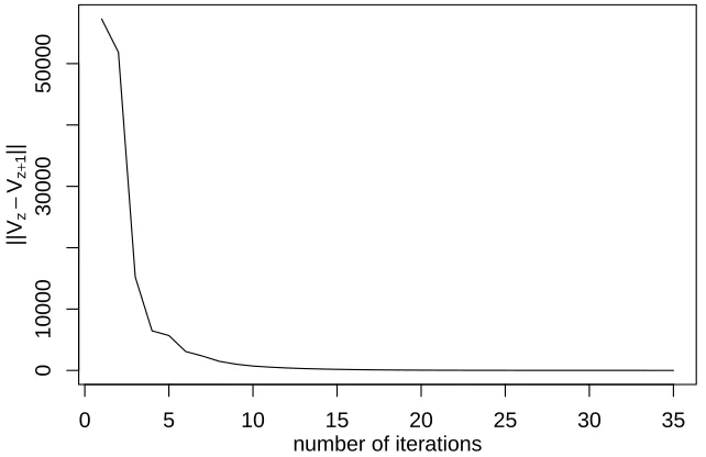
When the cardinality of B is 5000, we plot the evolving trace of||Vz−Vz+1||in Figure 3. Figure 3 shows that, even when

0 5 10 15 20 25 30 35

0

10000

30000

50000

||

Vz

−

Vz

+

1

||

[image:12.612.146.467.306.514.2]

number of iterations

Fig. 3: The evolving trace of||Vz−Vz+1|| when the sample size of belief points is 5000.

the size of belief points is large, the iteration process converges quickly: after 35 iterations, the distance ||Vz−Vz+1|| reduces

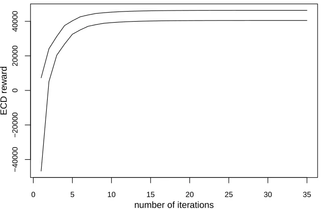
to 0.007. The time consumed for the whole procedure is 60844 seconds – around 16 hours. All computations were coded in R (version 3.2.2) on a PC with Intel Core i5-4590 CPU @3.30 GHz. After each iteration, we calculate the maximal ECD reward for each of the 5000 belief points. Then we record the minimum and maximum values of these 5000 maximal ECD rewards. To check the evolution of the decision process, we plot the 35 minimum ECD rewards and the 35 maximum ECD rewards in Figure 4. In Figure 4, after 15 iterations, the minimum ECD rewards and the maximum ECD rewards shape into two horizontal lines, implying that the value function has been stable.

Now the final value function should be very close to the underlying true value function. Therefore, we will use this final

value function for making maintenance decisions at an arbitrary time point. For example, if the belief state is(1,0,0,0), then

the optimal action is “do nothing”; the corresponding ECD reward is 46357.85. If the belief state is(0,0,0,1), then the optimal

action is “replace”; the corresponding ECD reward is 40385.84. Table I lists some belief points from the setB(rounded to four

decimal places) and the corresponding optimal actions and ECD rewards. Of course, these decision rules will change under different parameter settings.

B. Finite Planning Horizon

Whenwis finite, we re-encode the planning horizon with the time unit being one day. We setwto be 1095, corresponding

0 5 10 15 20 25 30 35

−40000

−20000

0

20000

40000

number of iterations

ECD re

w

[image:13.612.146.467.63.271.2]

ard

[image:13.612.133.475.319.430.2]

Fig. 4: The minimum and maximum ECD rewards of the 5000 belief points after each iteration.

TABLE I: A sample of belief points, their corresponding optimal actions and ECD rewards.

belief state optimal action corresponding ECD reward

(0.9972, 0.0028, 0.0000, 0.0000) 1 46316.40

(0.9965, 0.0035, 0.0000, 0.0000) 1 46306.04

(0.8714, 0.1286, 0.0000, 0.0000) 2 44454.43

(0.8160, 0.1840, 0.0000, 0.0000) 2 43634.51

(0.0031, 0.6803, 0.3165, 0.0001) 3 41215.31

(0.0001, 0.0390, 0.9457, 0.0152) 3 40574.81

(0.0000, 0.0003, 0.8488, 0.1509) 4 40498.43

(0.0000, 0.0000, 0.0000, 1.0000) 4 40385.84

u∗₁=78,u∗₂=85 andu∗₃=3. The transition matrices of actions 1 and 2 hence change slightly:

P(a=1) =



  

0.1111 0.7411 0.1430 0.0048

0 0.1111 0.7411 0.1478

0 0 0.1111 0.8889

0 0 0 1



   ,

and

P(a=2) =



  

0.1068 0.7413 0.1469 0.0050

0 0.1068 0.7413 0.1519

0 0 0.1068 0.8932

0 0 0 1



   .

u∗₄is a discrete random variable, taking values from{8,9,10,11,12} respectively with probabilities{0.1,0.23,0.34,0.23,0.1}. All the other parameter values are identical with what are given in the above section.

When w is finite, the size of the belief-point set depends on the value of w. In our example, it is not recommended to

simulate 5000 belief points as what we did for infinitew. If the belief-point setBcontains 5000 elements, the whole procedure

will take about 700 hours. We now randomly generate 1000 belief points by using Algorithm 1. We then in turn calculate V1095(·),V1094(·),V1093(·), . . ., until we arrive atV0(·). Apparently, the computational load is heavier than that whenwis infinite:

the computational time consumed is 166178 seconds – around 46 hours. At time 1095, the α-vector set contains only one

element: {(0,0,0,0)}, and the optimal action for every belief point is “do nothing”. Similarly, since the shortest duration of

all the actions is 3 days, the optimal actions for time points 1094, 1093 and 1092 are all “do nothing”, which is in tune with practice. Starting from time 1091 (backward), other maintenance actions are likely to be optimal for certain belief points. For

example, under the above parameter setting, at time 1091 if the belief point is (0,0.0272,0.9693,0.0035), then the optimal

action is “dose chemicals”, and the corresponding ECD reward is 70.5906.

{α₀k}k. Eachα vector in{α0k}k is associated with an optimal action. Now at time 0, if the decision maker’s belief point isbbb,

we chose from{α₀k}k the one that maximizes<α0k,bbb>:α ∗

0=arg max

α₀k∈{α₀k}k

<α₀k, bbb>. Then the optimal action to take at time 0 is the action associated with α₀∗, and the ECD reward by taking this action is approximately<α₀∗, bbb>. Likewise, if the

parameter setting does not change, then at any decision-making time pointz(1≤z≤1095), we all use{α_zk}k to approximate

the underlying true value function. With zapproaching to 1095 (and hence the planning horizonwis not large), we can refine

the α vector set by expanding the belief-point setB.

To check the evolution of the approximating value function, at each time point, we calculate the maximal ECD reward for each of the 1000 belief points. Then we record the minimum and maximum values of these 1000 maximal ECD rewards. We plot the 1096 minimum ECD rewards and the 1096 maximum ECD rewards in Figure 5. It is observed that the minimum

0 200 400 600 800 1000

0

10000

20000

30000

40000

time (day)

minim

um ECD re

w

ard

0 200 400 600 800 1000

0

10000

20000

30000

40000

time (day)

maxim

um ECD re

w

[image:14.612.147.464.188.395.2]

ard

Fig. 5: The minimum and maximum ECD rewards of the 1000 belief points for the time period [0, 1095].

ECD reward and maximum ECD reward increase rapidly at first (for example, during the time period [800, 1095]). If both the minimum ECD reward and the maximum ECD reward do not increase, then we can infer that the approximating value function has become stable. Yet, in Figure 5, from time 400 backward to time 0, the minimum ECD reward and maximum ECD reward are still increasing. To see this, we plot the minimum ECD rewards and the maximum ECD rewards over the

time period [0, 400] in Figure 6. Figures 5 and 6 demonstrate that withzevolving from 1095 backward to 0, the elasticity of

0 100 200 300 400

40465

40475

40485

40495

time (day)

minim

um ECD re

w

ard

0 100 200 300 400

46320

46330

46340

46350

time (day)

maxim

um ECD re

w

ard

Fig. 6: The minimum and maximum ECD rewards of the 1000 belief points for the time period [0, 400] when w=1095.

[image:14.612.147.466.500.707.2]

We now increase w to be 1825, corresponding to five years. The value functions for the time period [730, 1825] will be identical with what we have obtained. Hence we start from time 729 backward to time 0. The iterative procedure stops when

z goes back to 0, and then we approximate the underlying true value function by the set {α₀k}k. The computational time

consumed is 114425 seconds – around 31 hours. Likewise, we plot the minimum and maximum ECD rewards of the 1000 belief points for the time period [0, 729] in Figure 7. Figure 7 shows that over the time period [0, 729], both the minimum

0 200 400 600

40494.0

40494.2

40494.4

time (day)

minim

um ECD re

w

ard

0 200 400 600

46350.9

46351.1

46351.3

time (day)

maxim

um ECD re

w

[image:15.612.147.465.135.341.2]

ard

Fig. 7: The minimum and maximum ECD rewards of the 1000 belief points for the time period [0, 729] when w=1825.

ECD reward and the maximum ECD reward almost do not change. We can claim that the approximating value function has

become stable. Therefore, if we want to study a planning horizon of, say, ten years, we might just use{α₀k}k to approximate

all the true value functions for the first five years. There is no need to calculate the α vector set from time 3650 backward to

time 0.

VI. CONCLUSIONS

In this paper, we studied the continuous-observation POSMDP which is a natural tool for the maintenance optimization problem of discrete-state systems. We reasoned, via Properties 1 and 2, why the point-based value iteration algorithm is an efficient method for approximating the true value function. We also addressed several practical issues on incorporating different maintenance actions into the POSMDP model. For practical implementation, we studied both finite planning horizon and infinite planning horizon. While the general framework introduced may face computational challenges, we have investigated cases of practical interest in which it remains quite tractable. The numerical study showed that, when the planning horizon is infinite, the value iteration procedure converges quickly; when the planning horizon is finite, even if we consider a long planning horizon, the computational load is still acceptable. Hence, we say that the continuous-observation POSMDP model is of application value in the area of machine maintenance. The work developed in this paper can also be applied to problems in the area of reinforcement learning, where Markov decision process is a topic of great interest.

This work can be enriched in several ways. We think two challenging avenues of research are particularly promising.

• In this work, we only study one system. Yet, in some cases, maintenance decision making may concern several interactive

systems. Take the water utility for example. A water treatment works typically has several RGFs. Though these RGFs are independent of each other, if one of the RGFs fails, the other RGFs have to bear the additional working load. Consequently, the deteriorating behavior of these working RGFs will change. One solution to this problem is to add another action, called “add workload”. The time to take this action depends on the time at which an RGF fails.

• Another common action in machine maintenance is inspection, which will reveal the true state of the maintained machine.

Recall that one distinctive feature of POSMDP is the partial observability. Yet, via an inspection, the decision process changes from POSMDP to SMDP, and, whenever the action is not inspection, the decision process changes back to POSMDP. Incorporating inspection into POSMDP is an open problem of interest.

APPENDIXA

PROOF OF THECONTINUITY OF THESET{α_zk}k

We now prove that{α_zk}k is a continuous set by utilizing an idea proposed by [32]. If{α_z+k ₁}k is a finite set, then the belief

within a region for a single indexk. We letα_z+k ₁(∆)denote the region corresponding to the vectorα_z+k ₁; that is, the maximizing vector for all the belief points within α_z+k ₁(∆)isα_z+k ₁. With ¨bbbz,aandu being fixed, all observations that lead to belief states

llla(bbb¨z,u,o)falling withinα_z+k ₁(∆)can be aggregated into one meta observationOk(bbb¨z,a,u):

O_k(bbb¨z,a,u) ={o∈O|α_z+k ₁=arg max

{α_z+k₁}k

<α_z+k ₁, llla(bbb¨z,u,o)>}.

Then we have

Z

O

Pr(U_z=u,O¨z+1=o|bbb¨z,A¨z=a)exp(−θu)Vz+1(llla(bbb¨z,u,o))do

=exp(−θu)

∑

k Z

Ok(bbb¨z,a,u)

Pr(U_z=u,O¨z+1=o|bbb¨z,A¨z=a)<αz+k 1, llla(bbb¨z,u,o)>do

=exp(−θu)

∑

k Z

Ok(bbb¨z,a,u) n

∑

i=1

α_z+k ₁(i)

n

∑

j=1

¨

b_zjfji(u;a)gi(o;a)pji(a)do

=exp(−θu)

n

∑

j=1

"

∑

k n

∑

i=1

α_z+k ₁(i)fji(u;a)gi(Ok(bbb¨z,a,u);a)pji(a) #

¨ b_zj,

where

gi(Ok(bbb¨z,a,u);a) = Z

Ok(bbb¨z,a,u)

gi(o;a)do.

The value functionVz(bbb¨z)can be written as

Vz(bbb¨z) =max

a∈A





 n

∑

j=1

¨ b_zj



R¯a_z(j) +

w−tz

Z

0

exp(−θu)

∑

k n

∑

i=1

α_z+k ₁(i)fji(u;a)gi(Ok(bbb¨z,a,u);a)pji(a)du 

 





. (12)

To prove that {αzk}k is a continuous set, we only need to prove that the bracketed quantity changes continuously with ¨bbbz.

Recall that, the region Ok(bbb¨z,a,u)is defined as follows:

Ok(bbb¨z,a,u) ={o∈O|llla(bbb¨z,u,o)∈αz+k 1(∆)}.

From Equation (2) we know that, with aand ubeing fixed,llla(bbb¨z,u,o)is a continuous function of both ¨bbbz ando. Therefore,

the boundary of the regionOk(bbb¨z,a,u)changes continuously with ¨bbbz. Then it follows thatgi(Ok(bbb¨z,a,u);a)(and, consequently,

the bracketed quantity) is a continuous function of ¨bbbz.

APPENDIXB

PROOF OFPROPOSITION2

The Bellman backup operatorH can be re-written asHVz+1(bbb¨z) =max

a∈AH

a_V

z+1(bbb¨z)with

HaVz+1(bbb¨z) =<R¯az,bbb¨z>+ +∞ Z

0

Z

O

Pr(U_z=u,O¨z+1=o|bbb¨z,A¨z=a)exp(−θu)Vz+1(llla(bbb¨z,u,o))dodu

Assume that|Vz−Uz|is maximized at pointbbb:

||Vz−Uz||=|Vz(bbb)−Uz(bb)|b =|HVz+1(bbb)−HUz+1(bbb)|.

Denote as ˆa the optimal action for HVz+1 atbbb, and ˇa the optimal action forHUz+1 atbbb. Assuming HVz+1(bbb)≥HUz+1(bbb), then it holds that

|HVz+1(bbb)−HUz+1(bbb)|=HaˆVz+1(bbb)−HaˇUz+1(bbb).

Since HaˆUz+1(bbb)≤HaˇUz+1(bbb), we have

in which

HaˆVz+1(bbb)−HaˆUz+1(bbb)

=

+∞ Z

0

Z

O

Pr(Uz=u,O¨z+1=o|bbb¨z=bbb,A¨z=a)exp(−ˆ θu)[Vz+1(lllaˆ(bbb,u,o))−Uz+1(lllaˆ(bbb,u,o))]dodu

≤

Z +∞

0

Z

OPr(Uz=u,

¨

Oz+1=o|bbb¨z=bbb,A¨z=a)ˆ exp(−θu)||Vz+1−Uz+1||dodu

=

Z +∞

0

Pr(Uz=u|bbb¨z=bbb,A¨z=a)ˆ exp(−θu)du

||Vz+1−Uz+1||.

Since the bracketed quantity is strictly smaller than one, we have ||Vz−Uz||<||Vz+1−Uz+1||.

Now assume thatbbb is an arbitrary point. ˆa is the optimal action forHVz+1atbbb, and ˇa is the optimal action forHUz+1 atbbb. IfVz+1≥Uz+1, then,∀ uando,Vz+1(lllaˇ(bbb,u,o))≥Uz+1(lllaˇ(bbb,u,o)). By taking integration we have

Z +∞

0

Z

OPr(Uz=u,

¨

Oz+1=o|bbb¨z=bbb,A¨z=a)exp(−ˇ θu)Vz+1(lllaˇ(bbb,u,o))dodu

≥

Z +∞

0

Z

OPr(Uz=u,

¨

Oz+1=o|bbb¨z=bbb,A¨z=a)exp(−ˇ θu)Uz+1(lllaˇ(bbb,u,o))dodu.

Consequently,

Vz(bbb) =HVz+1(bbb) =HaˆVz+1(bbb)≥HaˇVz+1(bbb)≥HaˇUz+1(bb) =b HUz+1(bbb) =Uz(bbb).

Sincebbb is arbitrary, we haveVz≥Uz.

APPENDIXC

BELIEFPOINTBACKUP

By exemplifying the maintenance of an RGF, we give below the details for backuping a belief point. Since the sojourn time

distribution in our example does not depend on the current state or the following state, we might write f(u;a)for fji(u;a).

A. Infinite Planning Horizon

If w= +∞, the double integral in Equation (9) can be simplified:

Z +∞

0

Z 1

0

exp(−θu) max

{α_z+k₁}k

( _n

∑

j=1

" _n

∑

i=1

α_z+k ₁(i)fji(u;a)gi(o;a)pji(a) #

¨ b_zj

)

dodu

=

+∞ Z

0

exp(−θu)f(u;a)du

1

Z

0 max {α_z+k₁}k

{

n

∑

j=1

[

n

∑

i=1

α_z+k ₁(i)gi(o;a)pji(a)]b¨zj}do.

Here, we have replaced the supremum with the maximum, since the α-vector set in Algorithm 3 is finite. The first integral

w.r.t. u can be readily calculated; the second integral can be re-written into

Z 1

0 max {α_z+k ₁}k

<δ_ka(o),bbb¨z>do,

whereδ_ka(o) = (δ_ka₁(o),· · ·,δ_kna(o))and

δ_{k j}a(o) =

n

∑

i=1

α_z+k ₁(i)gi(o;a)pji(a), for 1≤j≤n.

Define

Ok(bbb¨z,a) ={o∈[0,1]|αz+k 1=arg max {αk_z+1}k

<δ_ka(o),bbb¨z>}.

Then the second integral can be further simplified:

Z 1

0 max {αk_z+1}k

( n

∑

j=1

" n

∑

i=1

αz+k 1(i)gi(o;a)pji(a) #

¨ b_zj

)

do=

∑

k n

∑

j=1

n

∑

i=1

αz+k 1(i)gi(Ok(bbb¨z,a);a)pji(a)b¨zj

=

n

∑

j=1

∑

k

n

∑

i=1

αz+k 1(i)gi(Ok(bbb¨z,a);a)pji(a)b¨zj

whereδ(bbb¨z,a) = (δ1(bbb¨z,a),· · ·,δn(bbb¨z,a))and

δj(bbb¨z,a) =

∑

k

n

∑

i=1

α_z+k ₁(i)gi(Ok(bbb¨z,a);a)pji(a), for 1≤j≤n.

Consequently, we have

Vz(bbb¨z) =max

a∈A<R¯

a

z+δ(bbb¨z,a)

Z +∞

0

exp(−θu)f(u;a)du, bbb¨z>, (13)

in which ¯Ra_z(j), 1≤j≤n, also can be simplified:

¯

Ra_z(j) =R1(j,a) + 1

θ

1−Eexp(−θUz)

bbb¨z,A¨z=a R2(j,a)

=R1(j,a) + 1

θ

1−

Z +∞

0

exp(−θu)f(u; a)du

R2(j,a).

To backup the belief point ¨bbbz, the most challenging thing is the calculation ofδ(bbb¨z,a). A traditional approach to backup ¨bbbz

is to identify, for every vectorα_z+k ₁, the mega observationOk(bbb¨z,a). Note thatOk(bbb¨z,a)may be composed of several separated

intervals. In the current work, instead of identifying the mega observation for each α vector, we indeed determine the optimal

α vector for each observation, which is accomplished by discretizing the [0, 1] interval. Specifically, for a large enough positive

integer r, define ov=2v₂−1_r for 1≤v≤r. Letαvdenote the maximizing α vector for observationov:

αv=arg max

{α_z+k ₁}k

( n

∑

j=1 " n

∑

i=1

α_z+k ₁(i)gi(ov;a)pji(a) #

¨ b_zj

)

.

Then, the second integral can be numerically approximated:

Z 1

0 max {α_z+k ₁}k

( n

∑

j=1 " n

∑

i=1

αz+k 1(i)gi(o;a)pji(a) #

¨ b_zj

)

do=1 r

r

∑

v=1

max {α_z+k₁}k

( n

∑

j=1