Deﬂation Technique to Accelerate the Convergence of Iterative Solver for the Wave Scattering Problem

(1)

Deflation Technique to Accelerate the Convergence

of Iterative Solver for the Wave Scattering Problem

A. H. Sheikh, A. G. Shaikh, Hisamuddin, Naeem Faraz, and Asif Ali

Abstract—An iterative solution method for the discrete high wavenumber Helmholtz equation is presented. The basic idea for solution, already presented in [1], is to develop a precondi-tioner which is based on a Helmholtz operator with a complex-valued shift for a Krylov subspace iterative method. The preconditioner which can be seen as a strongly damped wave equation in Fourier space, can be approximately inverted by a multigrid method. Extensive deflation and spectral analysis, as Krylov subspace methods depends upon eigenvalues, highlights in this paper. Findings in analysis are validated by numerical results.

Index Terms—Helmholtz equation, Multigrid Method, Pre-conditioning, Sparse linear systems, Deflation preconditioner.

I. INTRODUCTION

W

AVE scattering have many applications in physics, engineering and science. Examples include seismic imaging [1], [2], [3], [4], [5], radars, electromagnetism [6], bio medical imaging [7], (ultrasound), road-speed sensors etc. Wave scattering phenomena is mostly modeled by math-ematicians in the form of the Helmholtz equation [8], [9] and [10]. Solving Helmholtz equation requires the use of iterative methods. The Helmholtz equation in two dimensional (2D) or three dimensional (3D), the convergence is typically characterized by indefiniteness of the eigenvalues of the corresponding coefficient matrix. With such a property, an iterative method either basic or advanced, encounters conver-gence problems. The method usually converges very slowly or diverges [11]. There are very few choices of numerical methods to compute solution of very large sparse systems for many reasons, including memory, sparsity, heterogeneity of medium and indefiniteness. Indefiniteness limits the choice narrowly. The sparse direct solver have been used in [12], [13], [14] and [15]. They are heavily constrained with mem-ory and storage, hence are not practical for sufficiently large problems. The direct methods are not favorable for many obvious grounds, and they are too much time restrictions. They consume unaffordable memory for large problem which is under consideration. Discrete Helmholtz system, obtained by finite difference scheme, is approximated using Krylov subspace method. The preconditioner CSLP are tested with different shifts. Eigenvalue analysis of CSLP is given in

Manuscript received July 03, 2019; revised August 08, 2019.

A.H. Sheikh is with the Department of Mathematics & Statistics, QUEST Nawabshah, 67480 Pakistan e-mail: [email protected] .

A. G. Shaikh is with department of Mathematics & Statistics, QUEST Nawabshah 67480, Pakistan e-mail: [email protected].

Hisamuddin is with department of Mathematics, Shah Abdul Latif Uni-versity Khairpur, 66020 Pakistan e-mail: [email protected].

Naeem Faraz is with Center of International Program, Donghua University Shanghai PRC e-mail: [email protected] .

Asif Ali is with department of Basic Science & Related Studies, Mehran University of Engineering & Technology, Jamshoro 76062, Pakistan e-mail: [email protected] .

accordance with solver performance. For small frequency, CSLP performs better whereas increasing frequency, CSLP becomes impractical in terms of memory and computational time. Deflation technique is used to address these types of issues.

The Helmholtz equation can be read as

−∆2_{u(x, y)}₋_k2_{(x, y)u(x, y) =}_f_{(x, y),} ₍₁₎

where∆2₌ ∂2

(∂x2₎+

∂2

∂y2, andu(x, y)the unknown variable, defined on the unit square domain Ω = (0,1)×(0,1), K wave number. The wave numberkis related with wavelength λas

k(x, y) = 2π λ =

omega

c(x, y (2)

whereω= 2πF is angular velocity, F the wave frequency, λ=c(x,y_F ) the wavelength andc(x, y)is the speed of sound.

A. Model Problem

The Helmholtz problem considered this paper is non-homogeneous defined on the domain Ω = (x, y)×(x, y) wherex, y∈ (0,1). The wavenumber is constant, indepen-dent of geometry. The source function is given as

f(x, y) =δ(x, y) =δ(x−1/2, y−1/2). (3)

Withx, y∈(0,1)where Dirac delta function is given as

δ(x, y) =

(

+∞ x= 0, y= 0

0 x6= 0, y6= 0. (4)

This source functions is used to model the source centered at (1

2, 1

2). The domain is bounded by the Sommerfeld radiation

conditions [6] [1] [16], which are given as

∂u

∂η −ιku= 0. (5)

This models the propagation of wave from center outwards direction.Discretization: two lines. The resultant linear sys-tem is written as

Ahuh=fh. (6)

II. HELMHOLTZSOLVERS

Solving Helmholtz equation requires solution of resultant large sparse Linear System (6). For large, sparse matrix the Krylov subspaces are very popularchoice.The methods are developed on construction of iterants in the subspace.The space

Kj(A;r0) =Span{r0_{, Ar}0_{, A}2_r0_,_{· · ·}_{. . . A}(j−1)_r0_},

(2)

on construction the Krylov subspaces, a Conjugate Gradient (CG) [17],[18] [19] GMRES [20], CGS [21], Bi-CG [22], Bi-CGSTAB [23]and QMR are popular. For non-symmetric linear systems, Krylov subspace can be built from Arnoldi’s process, which leads to GMRES(Saad and Schultz, 1986). GMRES is optimal method; it reduces the 2-norm of the residual at the every iteration. GMRES, however, require long recurrences, which is usually limited by the available memory. A remedy is by restarting, which some-times lead to slow convergence or stagnation [24].

A. Preconditioning

In an iterative method preconditioning is often vital com-ponent in enhancing the convergence of iterations, partic-ularly when the system is large sized.. There are many iterative techniques for solving linear system. For large spare linear system, the convergence rate is always a concern for researchers; one can improve significantly the convergent rate by applying appropriate preconditioner. The convergence of iterative methods depends on eigenvalues of the coefficient matrix, it is often advantageous to use preconditioner that transfer the system to one with a better distribution of eigenvalues. The preconditioner is the key to successful iterative solver. In brief, to make linear system favorable for iterative solver, the coefficient matrix is scaled with a matrix Mcalled preconditioner. With choice of preconditionerMfor Linear System 6, where the inverse of M is relatively inexpensive to compute, and then the preconditioned system is M(−1)Au=M(−1)f is supposed to be favorable for iterative solver. A few preconditioners have been tried for the Helmholtz equation, for details see [10] [2] [4].

B. Complex Shifted Laplace Preconditioner

The Complex Shifted Laplace Preconditoner(CSLP) is the discrete Helmholtz operator in addition with a complex shift(a, ιb). The CSLP is preconditioner based on operator, in contrast to decomposition type preconditioners, which are matrix-based. The CSLP obtained by(finite difference) discretization of the shifted Helmholtz operator i.e.

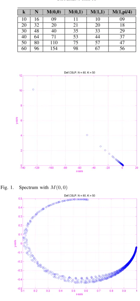
M(a, b) :=−∆−(a−ιb)k2, where a, b∈R, whereaandbare real and imaginary numbers respectively. The first precedent in operator based preconditioner for the Helmholtz equation was simple Laplace operator ∆, used without any shifts. It works well, until mesh size is small. For large size of mesh, convergence starts to stagnates, and alot of unwanted eigenvalues appear, as shown in Fig:1, which shows that for large mesh size this shift is not good choice. Later different shifts were introduced, with real as well as imaginary parts, and found to be effective. The number of iterations taken by GMRES preconditioned CLSP M(1, π/4) gorws with linear rate with wave number. This fact is illustrated by spectrum of preconditioned Helmholtz, as shown in Fig:2, where eigen values are getting more closer to orign. Some near-origin eigenvalues affect the convergence of solver. Deflation preconditioned, illustrated in next Sectin, is used to treat this drawback. A comparison of performance of CSLP with different shifts in given in Table I, where shift (1, π/4)is the one which outperforms rest of choices of shifts for small as well large wave numbers.

TABLE I

COMPARISON OFGMRES NUMBER OF ITERATIONS BYCSLPWITH DIFFERENT SHIFTS

k N M(0,0) M(0,1) M(1,1) M(1,pi/4)

10 16 09 11 10 09

20 32 20 21 20 18

30 48 40 35 33 29

40 64 71 53 44 37

50 80 110 75 57 47

[image:2.595.303.528.76.558.2]

60 96 154 98 67 56

Fig. 1. Spectrum withM(0,0)

III. DEFLATIONTECHNIQUE

Convergence of the Krylov subspace method is typically adversely affected by small eigenvalues, as seen in Fig: 2. The small eigenvalues need to be special treatment. Deflation is special type of preconditioner. Deflation is a technique commonly used to get rid of certain part of the spectrum, and to force the “unfair” eigenvalues not to participate in the Krylov iterative method. In order to develop deflation preconditioner, we consider the linear system

Ahuh=fh. (7)

For given a matrix Zh∈Cn×r, the deflation precondioners are the projections of type

(3)

where Qh = ZhA−2h1Z T

h and A2h = ZhTAhZh. Choice

of deflation vectors in matrix Zh forms an interest area

of research. Theoretically, eigenvectors gives ideal results, as they projects corresponding eigenvectors to zero. Since exact eigenvectors are impractical to compute, therefore many problem-specific possibilities have been explored. For the problem under consideration, few alternatives have been researched in [25], [9] and [26]. Getting motivation from property of resolving smaller error modes on coarser grids by multigrid, we choose multigrid coarsegrid operator as defla-tion matrixZhfor our problem. This deflation preconditioner

can be applied in combination with other preconditioners [27] and [28], and we have combined with CSLP as follows:

PhM(a, b)−h1Ahuh=PhM(a, b)−h1fh. (9)

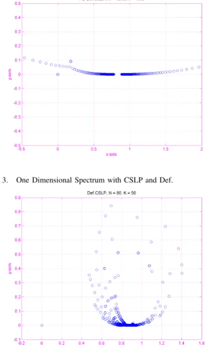
[image:3.595.69.269.316.477.2]

Next, we plot the spectrum of operator given in Eq: 9 in one-dimension as well as two-one-dimension in Fig: 3 and Fig: 4. These spectral plots show clustered behavior of eigenvalues of deflated CSLP-preconditioned matrix in one dimension and two dimension respectively.

Fig. 3. One Dimensional Spectrum with CSLP and Def.

IV. NUMERICALEXPERIMENTS

For all the experiments,u0 (zero vector) is used as initial guess. The mesh sizehis chosen such that for a wave number k, it satisfies relation kh ≤ 0.625 (equivalent to 10 grid

points per wave length). Iterations are stoppedn when the residul meets the tolerance

krhk ≤10−5.

A. Results

The first numerical result, using deflation, is presented in Table II, where CSLP is not used. This effort has been made to highlight affect of deflation preconditioner on its own. The readings show a substantial reduction in number of iterations and computational time. Subsequently, deflation is applied in combination with the CSLP, the first level preconditioner. A variety of shifts in CSLPj, in combination with defltaion, has been experimented and readings have been recorded and presented in Tables III, IV, V and VI for CSLP-shifts (0,0) , (0,1), (1,1) and (1,π₄) respectively. Such comparison is represented using consolidated bar plots given in Fig: 6, where bar representing iterations taken by solver preconditioned by CSLP and deflation is fairly smaller than the bar representing iterations taken by solver preconditioned by only CSLP. Comparison is performed with four different choices of shifts, comprehensible from figure. The two level preconditioned (CSLP and deflation perconditioner) solver is also tested for a very large wave number k = 200, and readings are presented in Table VII where inclusion of defltaion alongwith CSLP reduced the number of iterations significantly. Rate of reduction for shift (1,π₄) is 5 times. Lastly, the velocity potential for wave number ranging from k= 5tok= 30is plotted in Fig:5. Increasing wave number clearly highlights the need of more grid-points for large wave number.

TABLE II

NUMBER OF ITERATIONS BYGMRESANDDEFLATEDGMRES

k N Dim. of A GMRES It. Time Def GMRES It. Time

20 32 1089 74 00.79 13 00.11

40 64 4225 200 08.63 15 00.44

60 96 9409 405 51.95 17 01.10

80 128 16641 607 202.30 20 02.44

100 160 25921 782 362.79 24 04.36

TABLE III

NUMBER OF ITERATIONS BYCSLPANDCSLP-DEFLATION WITH

M(0,0)

k N Dim. A CSLPIt Time(S) CSLP-Def It Time(S)

20 32 1089 20 00.25 07 00.16

40 64 4225 71 02.86 10 00.70

60 96 9409 154 17.28 13 02.30

80 128 16641 257 66.02 16 05.26

100 160 25921 358 133.68 20 09.56

TABLE IV

M(0,1)

k N Dim of A CSLPIt Time (S) Def CSLP It Time(S)

20 32 1089 21 00.27 07 00.16

40 64 4225 53 02.15 10 00.75

60 96 9409 98 10.56 13 02.32

80 128 16641 137 28.70 16 05.18

[image:3.595.60.269.321.671.2]

(4)

TABLE V

M(1,1)

k N Dim A CSLP It Time Def. CSLP It Time

20 32 1089 20 00.26 07 00.16

40 64 4225 44 01.77 10 00.73

60 96 9409 67 07.07 13 02.28

80 128 16641 88 17.87 16 05.37

100 160 25921 108 33.44 21 10.16

TABLE VI

M(1, π/4)

k N Dim A CSLP It Time Def. CSLP It Time

20 32 1089 18 00.24 07 00.16

40 64 4225 37 01.49 10 00.74

60 96 9409 56 05.84 13 02.27

80 128 16641 73 14.54 16 05.09

100 160 25921 88 26.88 20 09.64

TABLE VII

NUMBER OF ITERATIONS BYCSLPANDCSLP-DEFLATION,DIFFERENT SHIFTSM(a, b)

CSLPM(a, b) Dim A CSLP It t(s) D-CSLP It t(s)

M(0,0) 103041 948 1681 48 107

M(0,1) 103041 349 542 49 108

M(1,1) 103041 208 267 49 86

M(1, π/4) 103041 169 248 49 83

V. CONCLUSION

In this paper, we discussed the ingredients of robust and efficient iterative solver for high wave number Helmholtz problems. Need of preconditioner is highlighted and a critical investigation of different preconditioners is presented. The CSLP preconditioner is applied and found to be very effective to enhance the convergence of Krylov subspace methods for small wave number problem. Increasing wave number stagnates convergence of CSLP preconditioned solver. The deflation is introduced and is used as a second-level in combination with CSLP, which not only pushes the small eigenvalues to origin ( unwanted eigenvalues ), also helps to achieve faster convergence fast. Specially when wave numbers are large, the deflation method takes less iterations as compared to the CSLP. It also reduces solve time for large wave number problem, which highlights the contribution of this paper.

REFERENCES

[1] A. Shaikh, G, A. H. Sheikh, A. Asif, and S. Zeb, “Critical Review of Preconditioners for Helmholtz Equation and their Spectral Analysis,”

Ind. Jour. Sc. Tech, vol. 12, no. 20, May 2019.

[2] Y. A. Erlangga, “A robust and effecient iterative method for numerical solution of Helmholtz equation,” PhD Thesis, DIAM, TU Delft, 2005. [3] R. E. Plessix, “A Helmholtz iterative solver for 3d seismic-imaging

problems,”Geophysics, vol. 72, pp. SM185–SM194, 2007.

[4] A. Sheikh, “Development of Helmholtz Solver Based on Shifted Laplace Preconditioner and a Multigrid Deflation Technique,” Delft University of Technology, The Netherlands, PhD Thesis, 2014. [5] A. H. Sheikh, D. Lahaye, and C. Vuik, “On the convergence of

shifted Laplace preconditioner combined with multilevel deflation,”

[image:4.595.326.526.58.224.2]

Numerical Linear Algebra with Applications, vol. 20, pp. 645–662, 2013.

[image:4.595.44.295.67.428.2]

Fig. 5. Velocity Potential of App. Sol. Increasing wavenumber

Fig. 6. Bar Iterative Comparison of CSLP and CSLP-Def.ofM(a, b)

[6] J. Berenger, “A perfectly matched layer for the absorption of elec-tromagnetic waves,”Journal of Computational Physics, vol. 114, pp. 185–200, 1994.

[7] S. Operto, J. Virieux, P. Amestoy, J. L’Excellent, L. Giraud, and H. Ali, “3d finite-difference frequency-domain modeling of visco-acoustic wave propagation using a massively parallel direct solver: A feasibility study,”Geophysics, vol. 72, no. 5, pp. SM195–SM211, 2007. [Online]. Available: http://dx.doi.org/10.1190/1.2759835 [8] A. Bayliss, C. I. Goldstein, and E. Turkel, “An iterative method for

the Helmholtz equation,”Journal of Computational Physics, vol. 49, pp. 443 – 457, 1983.

[9] A. H. Sheikh, C. Vuik, and D. Lahaye, “A scalable Helmholtz solver combining the shifted Laplace preconditioner with Multigrid deflation,” DIAM, TU Delft Netherlands, Tech. Rep. 11-01, 2011. [10] Y. A. Erlangga, “Advances in Iterative Methods and Preconditioners

for the Helmholtz Equation,”Archives of Computational Methods in Engineering, vol. 15, pp. 37–66, 2008.

[11] A. H. Sheikh, C. Vuik, and D. Lahaye, “Fast iteratie solution methods for teh Helmholtz equation,” DIAM, Delft University of Technology, The Netherlands, Tech. Rep. 09-11, 2009.

[12] P. Concus and G. H. Golub, “Use of Fast Direct Methods for the Efficient Numerical Solution of Nonseparable Elliptic Equations,”

SIAM J. Numer. Anal., vol. 10, pp. 1103–1120, 1973.

[13] L. Conen, V. Dolean, R. Krause, and F. Nataf, “A coarse space for heterogeneous Helmholtz problems based on the Dirichlet-to-Neumann operator,” Journal of Computational and Applied Mathematics, vol. 271, no. 0, pp. 83 – 99, 2014. [Online]. Available: http://www.sciencedirect.com/science/article/pii/S0377042714001800 [14] T. A. Davis,Direct Methods for Sparse Linear Systems (Fundamentals

of Algorithms 2). Philadelphia, PA, USA: SIAM, 2006.

[15] L. Giraud, D. Ruiz, and A. Touhami, “A Comparative Study of Iterative Solvers Exploiting Spectral Information for SPD Systems,”SIAM J. Sci. Comput., vol. 27, no. 5, pp. 1760–1786, 2006.

(5)

Helmholtz equation,”Computer Methods in Applied Mechanics and Engineering, vol. 163, no. 1, pp. 343–358, 1998.

[17] S. F. Ashby, T. A. Manteuffel, and P. E. Saylor, “A taxonomy for conjugate gradient methods,”SIAM J. Numer. Anal., vol. 27, no. 6, pp. 1542–1568, 1990.

[18] M. R. Hestenes and E. Stiefel, “Methods of Conjugate Gradients for Solving Linear Systems,”Journal of Research of the National Bureau of Standards, vol. 49, no. 6, pp. 409–436, Dec. 1952.

[19] G. H. Golub and D. P. O’Leary, “Some history of the conjugate gradient and Lanczos methods,”SIAM Rev., vol. 31, no. 1, pp. 50– 102, 1989.

[20] Y. Saad and M. H. Schultz, “GMRES: a generalized minimal residual algorithm for solving nonsymmetric linear systems,”SIAM J. Sci. Stat. Comput., vol. 7, no. 3, pp. 856–869, 1986.

[21] Y. Saad, “A Flexible Inner-outer Preconditioned GMRES Algorithm,”

SIAM J. Sci. Comput., vol. 14, no. 2, pp. 461–469, Mar. 1993. [Online]. Available: http://dx.doi.org/10.1137/0914028

[22] G. A. Watson, Ed., Numerical Analysis, ser. Lec-ture Notes in Mathematics. Berlin, Heidelberg: Springer Berlin Heidelberg, 1976, vol. 506. [Online]. Available: http://link.springer.com/10.1007/BFb0080109

[23] H. A. van der Vorst, “Bi-CGSTAB: A Fast and Smoothly Converging Variant of Bi-CG for the Solution of Nonsymmetric Linear Systems,”

SIAM J. Sci. and Stat. Comput., vol. 13, no. 2, pp. 631–644, Mar. 1992. [Online]. Available: http://epubs.siam.org/doi/10.1137/0913035 [24] R. B. Morgan, “A Restarted GMRES Method Augmented with Eigen-vectors,”SIAM J. Matrix Anal. Appl., vol. 16, pp. 1154–1171, 1995. [25] Y. A. Erlangga and R. Nabben, “Algebraic Multilevel Krylov

Meth-ods,”SIAM Journal on Scientific Computing, vol. 31, pp. 3417–3437, 2009.

[26] A. Sheikh, D. Lahaye, L. Garcia Ramos, R. Nabben, and C. Vuik, “Accelerating the Shifted Laplace Preconditioner for the Helmholtz Equation by Multilevel Deflation,” J. Comput. Phys., vol. 322, no. C, pp. 473–490, Oct. 2016. [Online]. Available: https://doi.org/10.1016/j.jcp.2016.06.025

[27] Y. A. Erlangga and R. Nabben, “Deflation and Balancing Precondition-ers for Krylov Subspace Methods Applied to Nonsymmetric Matrices,”

SIAM J. Matrix Anal. Appl., vol. 30, pp. 684–699, 2008.