Concentration Polarization pdf

(1)

Vacuum permeate An alternative method to pro-duce a pressure drop is the use of a vacuum on the membrane permeate. This has been shown to be highly effective in laboratory settings. However, the economics are not favourable for the large scale production of inexpensive components. Nevertheless, vacuum permeate systems may prove viable for small, high value-added systems.

Batch versus continuous Continuous reactor sys-tems are preferred; they require less down time and have higher production rates than batch systems of similar size. However, as previously detailed, if the role of the membrane is to remove a product component, the available partial pressure difference is limited and the process will always be working with a very limited pressure drop that will require very large mem-brane areas. Batch and semi-batch processes allow the system to develop some limited partial pressure dif-ference before membrane separation is attempted.

Membrane Degradation

The stability of the membrane is another important consideration. Ideally, for integrated systems, the membrane should be stable in all possible reaction environments: catalyst activation, normal reaction, catalyst regeneration and any thermal cycling experi-enced upon transitions. This presents speciRc chal-lenges for each system and there are few materials that can satisfy all of these requirements. Thus, special engineering solutions are necessary. Even if the membrane material can fulRl these speciRcations, the many components needed to produce a mem-brane reactor module may not.

Future Possibilities

Organic Separations

A great deal of research is currently focusing on the development of membranes (either polymeric,

inor-ganic, or hybrids of the two) for the selective separ-ation of liquid organic mixtures. If this research is successful, it will allow for incorporation into liquid-phase membrane reactors.

Control of Reactant Addition for Intermediate Product Recovery

A second area of immense current research activity is the development of oxygen-permeable membranes to inSuence the conversion of methane to either meth-anol or syn gas. The goal in these processes is a mechanism for the conversion of natural gas to a transportable liquid that may be further converted to high valued products. Current research has shown that membranes can be developed and that the appropriate catalysts are available for these conver-sions. Many engineering challenges lie ahead. These membrane reactor processes operate in excess of 7003C (sometimes much higher). Sealing these ce-ramic membranes into a housing remains a limita-tion. Further, the thermal stresses, which develop when cycling from 25 to '7003C, may result in membrane damage. While these are complex prob-lems, the incentive to succeed is large and numerous research efforts continue in this area.

Concentration Polarization

H. Wijmans, Membrane Technology and Research, Inc., Menlo Park, CA, USA

Copyright^ 2000 Academic Press

Introduction

All membrane separation processes are accompanied by a phenomenon called ‘concentration polarization’

(2)

[image:2.568.53.279.548.671.2]

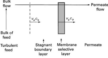
Figure 1 Schematic of the boundary layer adjacent to the

membrane surface. If cp'cb: component is enriched in

per-meate. Ifcp(cb: component is depleted in permeate.

Therefore, minimizing concentration polarization is one of the most important objectives in designing and engineering membrane separation systems.

Mathematical Description of

Concentration Polarization

The velocity proRle of a Suid Sowing in a channel is not constant across the thickness of the channel, because of friction at the _Suid_}channel surface interface. The _Suid velocity decreases as the distance from the channel surface decreases. The same phenomenon occurs in the channels of a mem-brane module, and the resulting velocity gradient adjacent to the feed side of the membrane is charac-teristic of all membrane processes. To facilitate mass transfer analysis, the velocity gradient is usually rep-resented by a step function, and it is assumed that a stagnant boundary layer exists adjacent to the mem-brane. Any component permeating the membrane must Rrst pass through the boundary layer as illus-trated in Figure 1.

Although the boundary layer is stagnant in the direction of the feed bulk_Sow, the boundary layer is subject to convective_Sow perpendicular to the mem-brane surface which is generated by the permeate Sux. The convective transport of a component into the boundary layer from the bulk solution is given by the productvp)cp, wherevp(cm s\1) is the convective

velocity and cb (g cm\3) is the concentration in the

bulk of the feed. The rate at which the same com-ponent leaves the boundary layer is vp)cp, where

cp(g cm\3) is the permeate concentration. In general,

if separation is achieved,cpdoes not equalcb, and the

convectiveSows into and out of the boundary layer, generate a mass imbalance. This imbalance then forms a concentration gradient in the boundary layer, and the concentration gradient increases until dif-fusion of the component down the concentration

gradient is sufRcient to restore mass balance in the boundary layer.

At steady state, the sum of convective and dif-fusive transport in the boundary layer equals the amount permeated through the membrane. This steady state is expressed for each component by the equation:

vpci!Ddci/dx"Jwi [1]

where D (cm2_s_\1₎ _is _the _diffusion _coef_R

c-ient, x (cm) is the coordinate perpendicular to the membrane surface and Jw

i (g cm\2s\1) is the mass

Sux of i permeating through the membrane.

In liquid-phase separations (including pervapora-tion) concentrations are typically expressed as a weight fraction,wi"ci/ where (g cm\3) is the

density of the liquid. Assuming that the density of the feed is constant in the boundary layer:

vp)wi)!D)

dwi dx"J

w

i [2]

and assuming that the feed density is equal to the density of the permeate:

Jw

i"wp)Jwtot"wp)vp) [3]

where wp (g g\1) is the weight fraction of i in the

permeate andJw

tot(g cm\2s\1) is the combined mass

Sux of all components permeating the membrane. Combining eqns [2] and [3] and eliminating the den-sitygives:

vp)wi!D

dwi

dx"vp)wp [4]

which, integrated over the thickness (cm) of the boundary layer, yields the polarization equation:

wm!wp

wb!wp"

exp(vp)/D)

"exp(vp/kbl)

"exp(Jw

tot/)kbl) [5]

wherewmandwbare the weight fractions of i at the

membrane surface and in the bulk of the feed, respec-tively, and kbl"D/ (cm s\1) is the mass-transfer

coef_Rcient in the boundary layer.

(3)

[image:3.568.55.274.400.650.2]

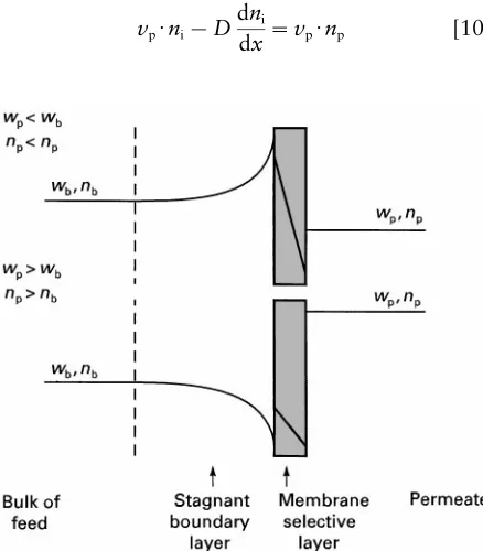
Figure 2 Schematic of the concentration polarization phenom-enon. The concentration profiles in the boundary layer result from the separation achieved by the membrane. The type of

concen-tration profile formed depends on the value ofwprelative towb(or

nprelative tonb).

to the volume fraction, assuming the gas mixtures are ideal. Starting again with eqn [1], the mole fraction

nican be substituted forciby using:

ni"ci)22 400)T/(Mi)pf)273) [6]

where 22 400 (cm3_{(STP) mol}_\1_{) is the molar volume}

of an ideal gas, T (K) is the gas temperature,

Mi(g mol\1) is the molecular weight of i, pf(bar) is

the feed gas pressure, and 273 K is the standard

temperature. Also, the volume Sux Jv

i

(cm3_{(STP) cm}_\2_s_\1_{) can be substituted for the mass}

SuxJw i using:

Jv

i"Jwi )22 400/Mi [7]

Elimination of the termMi/22 400 gives:

vp)ni)pf)273/T!D)pf)273/T

dni

dx"J

v

i [8]

SinceJv

i"np)Jvtotand:

vp"Jvtot)T/(pf)273) [9]

elimination of the termpf)273/Tgives:

vp)ni!D

dni

dx"vp)np [10]

Integrating eqn [10] in the same way as eqn [4] gives:

nm!np

nb!np"

exp(vp)/D)

"exp(vp/kbl)

"exp(Jv

tot)T/pf)273)kbl) [11]

wherenmandnbare the mole (or volume) fraction of

i at the membrane surface and in the bulk of the feed. Eqns [5] and [11] describe the concentration pro-Rles that develop in the boundary layer, as illustrated inFigure 2. Any component enriched in the permeate will be depleted in the boundary layer and any com-ponent depleted in the permeate will be enriched in the boundary layer.

Factors Determining the Extent

of Concentration Polarization

The ratio of the concentration of a component at the membrane interface to the concentration in the bulk of the feed is called the ‘concentration polarization modulus’ and is a measure of the inSuence of concen-tration polarization on the separation process. The following expression for the modulus can be obtained from eqn [5]:

wm

wb

" exp(vp/kbl)

1#Eo[exp(vp/kbl)!1]

[12]

where Eo"wp/wm is the intrinsic enrichment

achieved by the membrane (and equal to the actual enrichment if concentration polarization were ab-sent). An equation equivalent to eqn [12] but ex-pressed in mole fractions can be derived from eqn [11].

Eqn [12] allows the concentration polarization modulus to be calculated as a function of vp/kblfor

different values of the intrinsic enrichment fac-tors, Eo. The ratio vp/kbl is a Peclet number and is

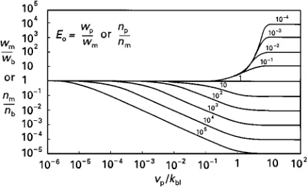
a measure of the inSuence of convection relative to the inSuence of diffusion in the boundary layer. The results of this calculation are shown in the very informative Figure 3, which conRrms that the con-centration polarization modulus is smaller than 1 (boundary layer depletion) if the permeating com-pound is enriched in the permeate and larger than 1 (boundary layer build-up) if the permeating com-pound is depleted in the permeate. The concentration polarization modulus increasingly deviates from unity as the ratiovp/kblincreases, that is, as theSux

(4)

[image:4.568.54.277.59.195.2]

Figure 3 Concentration polarization modulus,wm/wb, as func-tion ofvp/kblfor a range of values of the intrinsic enrichment factor Eo. Lines calculated through eqn [12]. This figure shows that

compounds that are enriched by the membrane (Eo'1) are more

affected by concentration polarization than compounds that are

rejected by the membrane (Eo(1).

of the feedSuid decreases. At high values for the ratio

vp/kbl, the concentration polarization modulus,

wm/wb, approaches the limiting value 1/Eo. At this

point, the boundary layer completely negates the sep-aration power of the membrane permeation step. The concentration polarization modulus also increasingly deviates from unity as the intrinsic enrichment in-creasingly deviates from unity, that is, as the separ-ation power of the membrane increases.

A striking feature of Figure 3 is the asymmetry with respect to enrichment and rejection. For example, when the term vp/kbl has a value of 10\1,

concentration polarization is essentially nonexistent for a component rejected by the membrane with an intrinsic enrichmentEoof 10\4. On the other hand,

concentration polarization is very severe for a com-ponent enriched by the membrane with an intrinsic enrichmentEoof 104. The reason for this asymmetry

is that the concentration polarization effect is generated by the difference in concentration be-tween the permeate and the feed, wp!wb"

wb(E!1), whereE"wp/wbis the actual enrichment

factor. It is clear that the absolute value ofwp!wbis

signiRcantly larger if E'1 than if E(1.

A second feature of the calculations shown in Figure 3 is that the concentration polarization modulus values are independent of the bulk concen-tration, wb. This means that at a constant

enrichment factor,E, the inSuence of concentration polarization is the same, no matter whether the com-ponent is present in the feed at a concentration of one part per hundred, one part per million, or one part per billion. Thus, concentration polarization does not necessarily affect components present at low concentrations more than components present at

higher concentrations. The primary requirement for signiRcant concentration polarization effects is a high value for the enrichment factor,E. However, becauseEhas an upper bound equal to 1/wb, a low

feed concentration is a secondary requirement for severe concentration polarization effects. This conRrms an empirical rule long held by membrane separation practitioners.

Transport Equations Incorporating

Concentration Polarization

As pointed out in the previous sections, concentration polarization primarily affects membrane per-meation by the change in composition at the mem-brane interface relative to the bulk of the feed mix-ture. To calculate the effect of concentration polarization on Sux and separation, the transport equation for the membrane can be combined with eqn [5] or eqn [11] to arrive at a set of equations that predict the permeate_Sux and composition.

Ultra_Rltration, nano_Rltration and reverse osmosis are membrane processes in which a solute is separ-ated from a solvent using a solute-rejecting mem-brane. Typically the permeate is essentially pure solvent, free of the solute. A simple but very effective transport equation developed for this situation is given below.

The pure solvent Sux Jw

solvent (g cm\2s\1) of the

membrane is given by:

Jw

solvent"P/Rm [13]

where P (bar) is the pressure difference applied across the membrane and Rm (bar cm2s g\1) is the

membrane resistance to the solvent. When a solute is present, the driving force for permeation is reduced by the osmotic pressure difference between the feed at the membrane interface and the permeate,

m(bar), therefore:

Jw

solvent"(P!m)/Rm [14]

Eqn [14] is called the ‘osmotic pressure model’, in which the osmotic pressure is a measure of the ther-modynamic work required to produce solvent from a solvent}solute mixture. Assuming that the permeate solute concentration is neglible:

m"a)wnm [15]

(5)

[image:5.568.60.271.54.257.2]

Figure 4 Solvent flux as a function of applied pressure as

calculated from eqn [17]. The flux observed with solvent}solute

mixtures is always less than the pure solvent flux. The deviation increases with increasing applied pressure, increasing solute con-centration, and decreasing mass-transfer coefficient in the bound-ary layer.

but equal to 2 or higher for macromolecular solutes. Combining eqn [15] with eqn [5] and assuming

wp"0 gives:

m"a)wnb)exp(n)Jwsolvent/kbl) [16]

and:

Jw

solvent"(p!a)wnb)exp(n)Jwsolvent/kbl))/Rm[17]

From eqn [17] it is clear that an increase in theSux

Jw

solventleads to an exponential increase in the osmotic

pressure and that the _Sux will increase less than linearly with the applied pressure. This means that any increase in driving force P will be negated at least in part by the increase in osmotic pressure. The general effect of pressure on Sux predicted by eqn [17] is illustrated inFigure 4and is in agreement with the vast majority of experimental data. As can be seen from Figure 4, the Sux observed with sol-vent}solute mixtures is always less than the pure solventSux, and the deviation increases with increas-ing applied pressure, increasincreas-ing solute concentration and decreasing mass transfer coefRcient in the boundary layer. Figure 4 also shows that at higher applied pressures the _Sux becomes essentially inde-pendent of the applied pressure. This is often ob-served in ultra_Rltration applications and is referred to as the limiting Sux. Eqn [17] predicts that under ‘limiting Sux’ conditions the Sux is independent of

the membrane resistance, which also has been con-Rrmed experimentally.

Gel Layer Formation

When the solute is a macromolecular compound such as a protein or a polymer, there is the possibility that the solute concentration at the membrane interface exceeds the gel concentration,wg, at which

concen-tration the solution is no longer a Suid. A gel layer thus forms at the membrane interface which creates an additional resistance to the permeationSux which consequently decreases. The Sux continues to de-crease until the solute concentration at the membrane interface equals the gel concentration, at which point steady state is reached. The_Sux at that point can be obtained from eqn [5]:

Jw

limit")kbl)ln

(wg!wp)

(wb!wp)

[18]

and becausewpis typically close to zero:

Jw

limit")kbl)ln(wg/wb) [19]

The steady-stateSuxJw

limitis called the ‘limitingSux’

because any increase in applied pressure will just result in a thicker gel layer and not in a higherSux. From eqn [19] it can be seen that the limiting_Sux as predicted by the gel layer model is independent of the applied pressure as well as the membrane resistance. Additionally, eqn [19] predicts a straight-line plot of

Jw

limitversus ln(wb) with a slope equal to!)kbl. All

these predictions have been conRrmed in a vast num-ber of ultraRltration experiments. Interestingly, the osmotic pressure model also predicts a limitingSux with the same attributes.

Approaches to Minimize

Concentration Polarization

(6)

potential employ spinning membranes or vibrating modules.

Dialysis in Medical Separations

W. R. Clark, Baxter Hemodialysis Research Lab., Wishard Hospital, Indianapolis, IN, USA

M. J. Lysaght, Brown University, Province, RI, USA

Introduction

Although haemodialysis (HD) as a therapy for ura-emia (kidney failure) wasRrst described early in the 1900s, its widespread use did not occur until the 1950s. At this time, Travenol Laboratories (now Bax-ter InBax-ternational) unveiled the ‘coil’ dialyser (‘arti_R -cial kidney’) in which tubes composed of cellophane membranes were wound around a support structure and immersed in a recirculated dialysis solution. Relative to contemporary models, the mass transfer efRciency of this type of dialyser was extremely poor, due to high mass transfer resistances in all three compartments (blood compartment, membrane, and dialysate compartment). In the early 1960s, solution mass transfer resistances were decreased with the introduction of parallelSow dialysers, in which sheet membranes were formed in a stacked conRguration. The improvement in dialysate-side mass transfer with these dialysers was particularly large because the dialy-sis solution contacted the membrane underSow condi-tions as opposed to the semi-batch operation of the coil dialyser. In addition, the membranes used in these devices were thinner in structure, providing less dif-fusive resistance than earlier versions. Although the earliest manufactured parallelSow dialysers were not disposable, design improvements permitted the pro-duction of disposable units by the late 1960s.

The last truly major development in haemo-dialysers occurred more than 30 years ago when the hollow Rbre artiRcial kidney was developed. Blood compartment mass transfer was reduced fur-ther with this design due to the high shear rate that could be achieved in the annular space of the hollow Rbre. Additional beneRts of the hollowRbre artiRcial kidney included an enhanced ability to control

trans-membrane pressure (see below) and a lower extracor-poreal blood volume. This type of dialyser is now used in virtually all HD treatments.

On a global basis, approximately 800 000 patients receive chronic haemodialysis therapy for the treat-ment of end-stage renal disease (ESRD) and this population is growing at a rate of 8}10% per annum. This Rgure represents approximately 85% of the ESRD population, with the remaining patients receiv-ing peritoneal dialysis. Numerous dialysis membrane and haemodialyser manufacturers are situated around the world, with the vast majority based in the three largest markets: United States, Western Europe and Japan.

The Haemodialysis Procedure

In addition to the dialyser, the other fundamental component of a HD system is a dialysis machine, which serves a number of purposes. First, it is equip-ped with a roller pump that delivers blood, usually at a rate of 200}500 mL min\1_{, from the patient to the}

dialyser and back to the patient. Second, the dialysis machine prepares dialysate by mixing (‘proportion-ing’) water and a concentrated bicarbonate solution in such a ratio that the dialysis_Suid produced is the same as that prescribed by a physician to meet the needs of an individual patient. The typical dialysate Sow rate is 500}800 mL min\1 _{and its major}