Constraint breeding during on line incremental learning

Constraint breeding during on-line incremental learning

⇤

Elliott Moreton

University of North Carolina, Chapel Hill [email protected]

Abstract

An evolutionary algorithm for simultaneously inducing and weighting phonological con-straints (Winnow-MaxEnt-Subtree Breeder) is described, analyzed, and illustrated. Imple-menting weights as sub-population sizes, re-production with selection executes a new vari-ant of Winnow (Littlestone, 1988), which is shown to converge. A flexible constraint schema, based on the same prosodic and au-tosegmental trees used in representations, is described, together with algorithms for mu-tation and recombination (mating). The al-gorithm is applied to explaining abrupt learn-ing curves, and predicts an empirical con-nection between abruptness and language-particularity.

1 Introduction

This paper aims to unite, within the framework of Harmonic Grammar (Legendre et al., 1990), two facts about phonological learning. One is that not all constraints can be innate; some are parochial and must be induced from language data (e.g., Prince and Smolensky 1993, 101), raising the question of

⇤_{The author is indebted to Brian Hsu, Katya Pertsova, and}

Jen Smith, Chris Wiesen of the Odum Institute at UNC-CH, and three anonymous SCiL reviewers for comments on previ-ous drafts. The paper benefited from audience comments on portions of Sections 6 and 7 at the Workshop on Computational Modelling of Sound Pattern Acquisition (University of Alberta, February 14, 2010), at an MIT departmental colloquium (April 9, 2010), and at the Workshop on Grammar Induction (Cornell University, May 14, 2010). The research was supported in part by NSF BCS 1651105, “Inside phonological learning”, to E. Moreton and K. Pertsova.

how new constraints are induced. The other is that phonological learning can be abrupt, in the sense that a flat learning curve can later accelerate, both in nature (Smith, 1973; Macken and Barton, 1978; Vihman and Velleman, 1989; Barlow and Dinnsen, 1998; Levelt and van Oostendorp, 2007; Gerlach, 2010; Becker and Tessier, 2011; Guy, 2014) and in the lab (Moreton and Pertsova, 2016), raising the question of what is going on during the period of apparent stagnation .

The proposed answer to both is that constraint in-duction and constraint reweighting happen simulta-neously via a single mechanism. Constraint weights are represented as sub-population sizes, i.e., the number of copies of a given constraint (“micro-constraints” in a “macro-constraint”). Error-driven reweighting of the macro-constraints happens when micro-constraints reproduce with fitness dependent on their contribution to error reduction. This pro-cess is shown to implement a modestly new in-cremental HG learning algorithm, Winnow-MaxEnt (§2), which is then analyzed (§§3, 4, 5). A flexible

prosodic and Feature-Geometric constraint schema, the Subtree Schema(§6), is used to add mutation and

recombination (§7), so that fitter constraint variants

can evolve and rapidly supersede their predecessors, leading to abrupt changes in performance (§8). The

paper ends with discussion (§9).

2 Weights as population sizes

The first step towards constraint breeding is to re-place constraint weights with population sizes so that differential reproductive success implements up- or down-weighting. Without changing the

har-69

mony of any candidate, we can replace any con-straint of weightwwithk“micro-constraints”, i.e.,

clones of that constraint, each with weight w/k.

Across an entire grammar, we can fix a parameter

⇣ to be the quantum of harmony, and replace every

(“macro-”) constraint of weightwwith a population

ofw/⇣microconstraints of fixed weight⇣.

Changes in weight of a macro-constraint re-sult from changes in population size of a constraint. When an error occurs, each micro-constraint produces an offspring with probability

(1 +✏)d_{, wheredis the difference between the}

win-ner’s and loser’s score on that constraint and✏is the

learning-rate parameter. If(1 +✏)d> kfor some

in-tegerk 1, the constraint produceskoffspring with

certainty, and another with probability(1 +✏)d k.

The new generation replaces the current generation. The weight update at the macro level is there-fore not described by a Perceptron-like algorithm, in which weights change by a fixed absolute in-crement, implementing gradient ascent on log-likelihood (Rosenblatt, 1958; Sutton and Barto, 1981; J¨ager, 2007; Boersma and Pater, 2016), but rather by one in which the increment is proportional to the weight, i.e., by a variant of Winnow-2 (Little-stone, 1988). This algorithm is analyzed in Sections 3–5 below.

The weights grow exponentially in the number of mistakes (Propositions 1 and 2, below), so a population explosion may threaten to overwhelm the learner’s limited computational substrate. That problem can be addressed using weight decay: On each update (or on each trial), the learner can delete each micro-constraint with a fixed probability, caus-ing the macro-constraint weights to decay by an amount proportional to their magnitude and slowing population growth. Alternatively, the decay rate can be adjusted dynamically, randomly deleting or du-plicating micro-constraints to maintain a fixed total micro-constraint population size.

3 The Winnow-MaxEnt algorithm

Winnow-MaxEnt, the learning algorithm induced by the constraint-breeding algorithm, is similar to Winnow-2 (Littlestone, 1988), but with the follow-ing differences. Winnow-MaxEnt (1) models k

-alternative forced choices rather than yes-no

clas-sification, (2) responds probabilistically rather than deterministically, and (3) supports non-binary con-straint scores. The original Winnow-2 was first sug-gested as a possible HG learner by Magri (2013). This section describes the two-alternative Winnow-MaxEnt. Generalization tok > 2 and to negative

constraints is discussed in Section 5 below.

Each ofnconstraints (macro-constraints) gives a

non-negative score to any candidate. The algorithm sees only the score vectors, and so is equally appli-cable to pure phonotactic learning (where each can-didate is a surface form and there are no faithfulness constraints) and to alternation learning (where each candidate is an input-output pair and there are faith-fulness constraints). We writexifor the score given

byCito Candidatex. Each constraintCihas weight

wi > 0, so that the state of the learner is described

by the weight vectorw= (w1, . . . , wn).

Given the experimenter’s intended winnerx+and

intended loser x , the learner chooses x+ _{with a}

probability that depends on the harmonies of the candidates. The version of the model discussed here uses the Luce choice rule applied to the exponenti-ated harmonies:

Pr(x+|x+, x ) = exp(

Pn

i=1x+i wi)

exp(Pn_i=1x+_i wi) + exp(Pni=1xi wi)

(1) This rule (Luce, 1959, 23) is an independently-justified model of human choice behavior across a wide range of domains (Bradley and Terry, 1952; Luce, 1977; Strauss, 1992; Macmillan and Creel-man, 2004). Its use with exponentiated harmonies yields a conditional Maximum Entropy (MaxEnt) model (Goldwater and Johnson, 2003; J¨ager, 2007; Hayes and Wilson, 2008). The losers (“negative evi-dence”) may be presented to the learner explicitly in the form of a 2AFC experimental trial, or implicitly in the form of an internally-generated candidate set. Ifx+is chosen, nothing changes. Ifx is chosen,

the weights of winner-preferring constraints grow, and those of loser-preferring constraints shrink, ac-cording to the update rule

w0_i=wi↵di (2)

where↵= 1+✏for some fixed learning-rate

4 Convergence of Winnow-MaxEnt

MaxEnt is different enough from Winnow-2 that convergence cannot be assumed on the basis of Littlestone (1988)’s proof for Winnow-2, though ideas from that proof are useful here. In fact, since the probability of an error cannot be zero, Winnow-MaxEnt does not converge at all, in the sense of ceasing to make mistakes. However, we will see that the error rate can be made arbitrarily small.

4.1 Consequences of the update rule

The Propositions presented in this subsection are de-rived from the update rule (Equation 2) and do not depend on the response rule, the candidate-set size, or the sign of the marks awarded.

We proceed as usual (Novikoff, 1963) by first as-suming that the target concept is representable in the learner, and then finding lower and upper bounds on a function of the weights in terms of the number of mistakes. LetDbe the (multi-)set of candidate pairs

used in the experiment. Each pair consists of an in-tended winner x+ _{and an intended loser x . The}

same pair may occur multiple times, and not all pos-sible pairs need occur. A candidate that is the posi-tive member of one pair may be the negaposi-tive mem-ber of another. Suppose that there exist nonnegative weights µ = (µ1, . . . , µn) and a µ such that for

every candidate pair(x+_{, x )2D,} n

X

i=1

µi(x+_i x_i )> µ>0 (3)

Proposition 1 (analogous to Littlestone (1988)’s Lemma 9). Let W = Pn_i=1wi, and let a

tar-get concept satisfying Inequality 3 be given. Let Aµ= µ/Pni=1µi. Then after thet-th update,

logW(t)>min

i (logwi(0)) +t·Aµlog(1 +✏) (4)

Proof. Taking the logarithm of Equation 2 yields

logw_i0 = logwi+ (x+_i x_i ) log↵. Hence n

X

i=1

µilogwi0 = n

X

i=1

µilogwi+(log↵) n

X

i=1

µi(x+i xi )

(5) Substituting from Equation 3 we have

n

X

i=1

µilogwi0 > n

X

i=1

µilogwi+ (log↵)· µ (6)

and so aftertupdates,

n

X

i=1

µilogwi(t)> n

X

i=1

µilogwi(0) + (log↵)· µ·t

(7) Since all the µi’s are nonnegative, the sum on the

left doesn’t get smaller if we replace all the weights with the largest weight, and the sum on the right doesn’t get larger if we replace all the weights with the smallest weight. Let i⇤ = arg max_iwi(t) and ˆ_{i= arg min}

iwi(0); then

logwi⇤(t) n

X

k=1

µk>logwˆ_i(0) n

X

k=1

µk+(log↵)· µ·t

(8) Since the µi’s are all nonnegative, we can divide

through by their sum to conclude that

logwi⇤(t)>logwˆ_i(0) +t·Aµ·log↵ (9)

SincelogW(t) = logPn_i=0wi(t)>logwi⇤(t), the

claim is proven.

Proposition 2. Let a target concept satisfying In-equality 3 be given. Let ⌃+ ₌ Pn

i=1x+i wi and ⌃ = Pn_i=1x_i wi for a given winner-loser pair (x+, x ). Then for any✏_1/(dmax 1),

logW(t)_logW(0) +✏_·

t 1

X

⌧=0

⌃+_{(⌧) ⌃ (⌧)}

W(⌧)

+t_· d

2 max✏2

1 (dmax 1)✏

(10)

Proof. From the update rule in Equation 2 plus the binomial theorem,

W0=W + n

X

i=1

(↵di _1)w i

=W +

n

X

i=1

(di✏+O(✏2))wi

=W +✏(⌃+ ⌃ ) +O(✏2)W

(11)

To bound the O(✏2_{) term explicitly, we rewrite}

Equation 11 as

W0 =W + X i|di>0

(↵di _1)w i+

X

i|di<0

(↵di _1)w i

(12) Since✏(⌃+ ⌃ ) = Pn_i=1✏diwi, we can rewrite

W0=W +✏(⌃+ ⌃ )

+ X

i|di>0

(↵di _{1 ✏d} i)wi

| {z }

Y

+ X

i|di<0

(↵di _{1 ✏d} i)wi

| {z }

Z

(13) By Theorem 2 of Mitrinovi´c (1970, p. 34),

(1 +x)n 1_ nx

1 (n 1)x (14)

forn > 1and 1 _ x _ 1/(n 1). This clearly also holds forn = 0andn = 1 as long asx 0.

Hence fordi 0and✏1/(dmax 1),

↵di _1 di✏

1 (di 1)✏ (15)

with strict equality ifdi = 0ordi= 1. Therefore,

Y _ X

i|di>0

di✏

✓

1 1 (di 1)✏

1

◆ wi

 X

i|di>0

di✏

✓

(di 1)✏ 1 (di 1)✏

◆ wi

(16)

Likewise,

Z = X

i|di<0

(↵ |di| _{1 +✏|d}

i|)wi ₍₁₇₎

Ifn, x 0, then by the binomial theorem,(1 +

x)n 1 +nx, so

(1+x) n 1 = 1

(1 +x)n 1 1

1 +nx 1 = nx

1 +nx

(18) Hence,

Z  X

i|di<0

✓

|di|✏

1 +|di|✏+|di|✏

◆ wi 

X

i|di<0

(_|di|✏)2 1 +|di|✏wi

(19) The sumY +Zis therefore bounded by

Y +Z _

n

X

i=0 max

( _{|di|(|di| 1)✏}2

1 (|di| 1)✏

|di|2✏2 1+|di|✏

)

wi (20)

Combining the larger numerator and smaller denom-inator to get a fraction that is larger than either, we have

Y +Z  n

X

i=1

d2_i✏2

1 (_|di| 1)✏

wi

 d

2 max✏2 1 (dmax 1)✏W

(21)

Combining Inequalities 13 and 21 yields

W0W ✓

1 +✏⌃

+ _⌃

W +

d2_max✏2

1 (dmax 1)✏

◆

(22) Sincelog(1 +x)x, we have

logW0_logW +✏⌃

+ _⌃

W +

d2 max✏2 1 (dmax 1)✏

(23) from which the proposition follows by summation from⌧ = 0to⌧ =t 1.

Proposition 3. Let a target concept satisfying In-equality 3 be given, and let Amax be the least

up-per bound onAµ over allµ. LetV = logW(0) mini(logwi(0)), and let a = (⌃+ ⌃ )/W for

a given winner-loser pair (x+, x ). Then for any

✓ >0, there exist✏✓ andt✓such that when

Winnow-MaxEnt is run with✏=✏✓,

1

t ·

t 1

X

⌧=0

a(⌧) Amax ✓ (24)

for allt t✓.

Proof. Propositions 1 and 2 together imply that for allt 0and✏1/(dmax 1),

✏

t 1

X

⌧=0

a(⌧) V +tAlog(1 +✏) td 2 max✏2 1 (dmax 1)✏

(25) Sincelog 1 +x x x2_/2,

1

t ·

t 1

X

⌧=0

a(⌧) A 1

2A✏

d2_max✏

1 (dmax 1)✏

V ✏t

(26) Sufficiently small✏and largetmake the right-hand side as close toAas desired.

To bound t✓, we note that the remainder in

In-equality 26 is bounded above by

f(✏, t) =1 2A✏+

d2_max✏

1 (dmax 1)✏+

V ✏t

<1

2A✏+

d2_max✏

1 dmax✏+

V ✏t

(27)

so thatf(✏, t)< g(dmax✏,1/t),

g(x, y) =F x+dmax x

1 x +

Gy

x (28)

f(✏, t) < ✓. Settingg(x, y) = ✓and solving for y

yields

y=h(x) = 1

G ✓

✓x F x2 dmax x 2

1 x

◆

(29) forx 2 (0,1). We want to choose x(= dmax✏) so

as to maximizey(= 1/t). The functionh(x)is hard

to maximize analytically, so instead we maximize a more tractable minoranti(x)to bound the maximum

ofh(x)below. Using the fact that1/(1 x)_1 + 2x,x2[0,1/2], we have

i(x) = 1

G ✓x F x

2 _d

max(x2+ 2x3) (30)

Thenh(x) i(x)for allx 2 (0,1/2].

Differentia-tion shows thati(x)attains a maximum at

x✓ =

p

(dmax+F)2+ 6dmax✓ (dmax+F) 6dmax

(31) Whatever the global maximum ofh(x)might be, it

is at least as big asi(x✓), i.e. maxx2(0,1)h(x) max_x2(0,1/2]h(x) h(x✓) i(x✓), which is

i(x✓) =

T+U2 ⇣pT +U2 _U⌘ 1 2T U 54V

(32) whereT = 6✓/dmaxandU = 1 +A/2d2max.

There-fore, there exist an✏✓=x✓/dmaxand at✓ = 1/i(x✓)

such that f(✏✓, t✓)  g(x✓, i(x✓)) = ✓. Thus,

t✓ = O(✓ 3/2). The smallest possible V occurs

when all the initial weights are equal, in which case

V = lognandt✓ =O(logn); i.e., the time bound

is not very sensitive to the number of constraints.

4.2 2AFC performance

This subsection addresses the question of how the bound on the relative harmony gap (Proposition 3) translates into a bound on 2AFC error probability. From Equation 1, the log-odds of choosing the cor-rect candidate is

log odds(x+_|x+, x ,w) = ⌃+ ⌃ =aW

(33) whereais defined as in Proposition 3. The

cumula-tive average log-odds of a correct response across all trials where an error actually occurred is therefore

L(t) = 1

t

t 1

X

⌧=0

a(⌧)W(⌧) (34)

where⌧ indexes errors as in Propositions 2 and 3.

Let✓be given and let✏✓ andt✓be as in Proposition

3, andt t✓. From Proposition 1, for any⌧ 0,

W(⌧) exp(min

i (logwi(0)) +Amax(log↵✓)⌧) min

i (wi(0)) exp(Amaxlog(↵✓)⌧) min

i (wi(0)) exp(Amax✏✓⌧)

(35) since1 +x logx. This lower bound on W(⌧)

is a strictly increasing function of ⌧. The same

is not necessarily true of a(⌧), but we can see

that for a fixed value of A(t) = (1/t)Pt_⌧=01 a(⌧),

the lower bound on L(t) is minimized when

a(0), a(1), . . . , a(⌧⇤)are as big as possible — i.e.,

equal todmax — and the rest of thea(⌧) are zero.

Thus ⌧⇤ = t·A(t)/dmax. To skirt complications

when ⌧⇤ is not an integer, we switch to a

continu-ous approximation, using the fact that Pn k=0ek

Rn 0 exdx:

L(t) 1

t Z ⌧⇤

0

dmaxW(⌧)d⌧

dmax

t Z ⌧⇤

0

µ0exp(Amax✏✓⌧)d⌧

µ0dmax

Amax✏✓ 1

t ✓

exp

✓ Amax✏✓

dmax tA(t)

◆

1

◆

(36) whereµ0 = mini(wi(0)). From Proposition 3, we

know thatA(t) Amax ✓, so

L(t) µ0dmax

Amax✏✓ 1

t ✓

exp

✓

Amax✏✓(Amax ✓)

dmax t

◆

1

◆

4.3 Simulation results

The analysis was checked by a simulation whose parameters were chosen to roughly approximate a typical Harmonic Grammar phonological analysis. For each replication of the simulation,n was

sam-pled uniformly from {2, . . . ,20_}, and dmax from {1,2,3,4}. Numbers m and r were uniformly

sampled from 4 to 64 and from 8 to 256, respec-tively. A weight vector µ of length n was made

by uniformly sampling each entry from the inter-val (0,1). The cells of an m_⇥n tableau

(candi-dates⇥constraints) were filled by uniformly

sam-pling each from { dmax, . . . ,0}, and one was

ran-domly (uniformly) chosen to be the most-harmonic positive stimulus, so long as it was not the most-or least-harmonic of all. The other candidates’ har-monies thus determined their positive/negative sta-tus. The least upper boundAmaxwas approximated

by maximizing Aµ over all µ consistent with the

concept using the quasi-Newton method of Byrd et al. (1995) as implemented in the optim func-tion of Version 3.2.2 of thestatspackage in R (R Core Team, 2015). A numberrof winner-loser pairs

was made by randomly sampling (uniformly, with replacement) from the positive and negative candi-dates, provided that some intended winners had less-than-perfect scores. A ✓ was sampled uniformly

from[1/32,1/8], ✏✓ was chosen as in Equation 31,

andt✓was chosen as in Equation 32. Initial weights

were all set to 1. Winnow-MaxEnt was trained un-til the learner’s cumulative average relative harmony gap (the left-hand side of Inequality 26) reached or exceeded Amax ✓/2, or until 5t✓ errors had

oc-curred. (If that criterion was already met before any training, the simulation was discarded and replaced.) In 10,000 replications, the bound of Inequality 26 always underestimated the cumulative average harmony gap at every time point (error) in every replication by a margin of at least 0.0823 (median, 0.9732). The bound of Inequality 32 always overes-timated the actual number of errors required to reach

Amax ✓by a factor of at least 3.93, and usually by

very much more (the median was a factor of 52.60). The bound in Inequality 37 always underestimated the actual log-odds att=t✓ by at least a margin of

1.084 (median, 280.3). Average-case performance in actual applications may therefore be much better.

5 Beyond 2AFC with positive constraints

Because the Luce choice rule describes how to choose one item out of a set of alternatives on the basis of nonnegative harmony values, k-AFC for k > 2 requires no amendment for positive

con-straints. For negative constraints, we let the alter-natives be, not individual candidatesxi 2 X,

com-peting to be the winning individual on the basis of their harmonieshw(xi), but rather sets ofk 1

can-didates Xi = X {xi}, competing to be the

los-ing set on the basis of their harmonies Hw(Xj) =

P

x2Xjhw(x) = (

P

x2Xhw(x)) hw(xj). Then

Pr(xi |X,w) =

exp P_x2Xhw(x) /exp(hw(xj))

Pk

j=1exp

P

x2Xhw(x) /exp(hw(xj))

=_Pkexp( hw(xi)) j=1exp( hw(xj))

(38) In other words, negative (penalizing) constraints can be implemented by simply inverting the sign of the marks awarded.

6 Constraints as representation subtrees

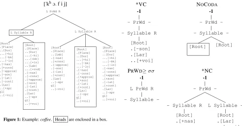
The next step is a constraint schema that enables breeding and mutation. We can define markedness constraints as subtrees of autosegmental representa-tions, such that every representation is itself a con-straint (Burzio, 1999). The representational system in the implemented model is a hierarchical prosodic and featural tree structure simplified from Gussen-hoven and Jacobs (2005, Ch. 5) by omitting feet and moras. Figure 6 shows an example.

A markedness constraint is a representation, rooted at a PrWd, which awards a mark to a can-didate for each time it matches part of that candi-date. Examples of familiar markedness constraints expressed in this schema are shown in Figure 2. The symbols L and R mark left and right constituent

boundaries.

["kh_{O. f i j]}

L PrWd R

L Syllable R

[image:7.612.73.564.70.325.2]

[Root] .[Place] ..[Dor] ...[+hi] ...[-bk] ...[-lo] .[-nas] .[+cons] .[-approx] .[-son] .[-lat] .[-cont] .[Lar] ..[+spr gl] ..[-voi] [Root] .[Place] ..[Dor] ...[-hi] ...[+bk] ...[+lo] ..[Lab] ...[+rnd] .[-nas] .[-cons] .[+approx] .[+son] .[-lat] .[+cont] .[Lar] ..[-spr gl] ..[+voi]

L Syllable R

[Root] .[Place] ..[Lab] .[-nas] .[+cons] .[-approx] .[-son] .[-lat] .[+cont] .[Lar] ..[-spr gl] ..[-voi] [Root] .[Place] ..[Dor] ...[+hi] ...[-bk] ...[-lo] .[-nas] .[-cons] .[+approx] .[+son] .[-lat] .[+cont] .[Lar] ..[-spr gl] ..[+voi] [Root] .[Place] ..[Dor] ...[+hi] ...[-bk] ...[-lo] .[-nas] .[-cons] .[+approx] .[+son] .[-lat] .[+cont] .[Lar] ..[-spr gl] ..[+voi]

Figure 1:Example:coffee. Heads are enclosed in a box.

with prosodic constituent structure, thus support-ing positional constraints; it accommodates non-adjacent dependencies; it allows variables (not dis-cussed here) for (e.g.) AGREE, OCP, and

reduplica-tion; and it provides continuity between constraints and representations (Golston, 1996; Burzio, 1999). The tree structure also lends itself to a recursive breeding algorithm, as described in the next section.

7 Mutation, recombination, and selection

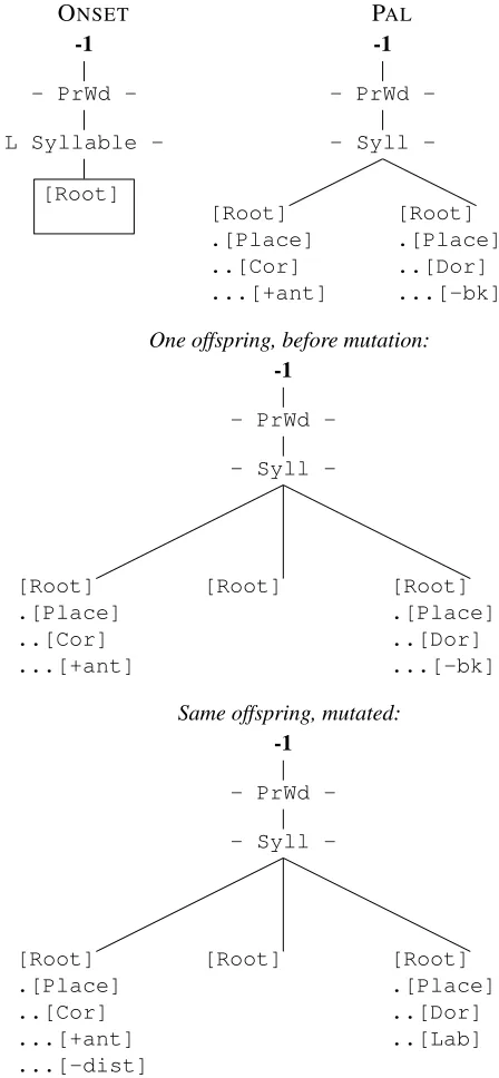
We now let the micro-constraints reproduce with variation, so that the Winnow-MaxEnt rule acts as a selective force in an evolutionary algorithm. Evo-lutionary algorithms have long been applied to prob-lems closely related to the ones addressed here, in-cluding evolving receptive fields for inputs to the single-layer perceptron (Nakano et al., 1995) and evolving tree structures (Cramer, 1985; Koza, 1989). Replication of mental representations with variation, recombination, and selection is a leading theory of human creativity in other domains (Simonton, 1999, 2004; Dietrich and Haider, 2015).

Each constraint which is chosen to breed is ran-domly paired with another chosen breeder of equal or greater fitness (reproductive probability). The two constraints are mated recursively. The offspring of two prosodic-category nodes randomly copies node-level properties (left and right anchors) from the

par-*VC NOCODA

-1

PrWd

-- Syllable R

[Root] .[-son] .[Lar] ..[+voi]

-1

PrWd

Syllable

-[Root] [Root]

PRWD *NC

-1

L PrWd R

Syllable

--1

PrWd

-- Syllable R

[Root] .[+nas]

L Syllable

-[Root] .[Lar] ..[-voi]

Figure 2:Some familiar markedness constraints in the Subtree Schema: *VC, final-obstruent devoicing (Ito and Mester, 2003); NOCODA(Prince and Smolensky, 1993); a constraint enforcing a disyllabic minimal prosodic word; *NC (Pater, 2004).

ents. Immediate dependents of each parent node are randomly paired, preserving left-to-right order, and leaving some dependents unpaired if one par-ent node has more than the other. Each pair of dependents then breeds to make one node in the offspring. An unpaired dependent is either inher-ited intact or deleted, with probability 1/2. The offspring of paired compatible unary-feature nodes (e.g., [+Cor] bred with [+Cor]) is computed analo-gously: Subfeature nodes common to both parents are paired and bred recursively; unpaired nodes are either copied intact or deleted, with probability 1/2. The offspring of paired compatible binary-feature nodes (e.g., [+voice] bred with [ voice]) is identi-cal to each of the parents with probability 1/2. An example is shown in Figure 3.

invert-ONSET PAL

-1

PrWd

L Syllable

-[Root]

-1

PrWd

Syll

[image:8.612.76.300.72.556.2]

-[Root] .[Place] ..[Cor] ...[+ant]

[Root] .[Place] ..[Dor] ...[-bk]

One offspring, before mutation:

-1

PrWd

Syll

-[Root] .[Place] ..[Cor] ...[+ant]

[Root] [Root]

.[Place] ..[Dor] ...[-bk]

Same offspring, mutated:

-1

PrWd

Syll

-[Root] .[Place] ..[Cor] ...[+ant] ...[-dist]

[Root] [Root]

.[Place] ..[Dor] ..[Lab]

Figure 3:Breeding and mutation, illustrated with parents ON-SET(`a la Smith 2003, 2012) and PAL(McCarthy, 1999).

ing the coefficient on a binary feature. The probabil-ity of each is controlled by a separate parameter. A macro-constraint thus becomes an equivalence class of formally diverse micro-constraints which assign the same marks to all of the candidates.

8 Constraint breeding in practice

The combination of Winnow-MaxEnt with the Sub-tree Schema is illustrated using an artificial

phono-tactic pattern. Candidates were the initial sylla-bles from the stimuli of Saffran and Thiessen (2003, 494). The positive stimuli (winners) had the form

{p, t, k_}V_{b, d, g_}and the negative stimuli (losers)

{b, d, g_}V_{p, t, k_}. The population size was fixed at n = 1000(micro-)constraints, which initially were

identical clones that gave 1mark to every PrWd.

On each trial, a random candidate pair was presented for 2AFC judgement. When a mistake happened, the quantityri =↵x

+

i xi was calculated for each

con-straintCi. If ri 1, the constraint made one

off-spring with certainty, then another with probability

1 ri. Ifri <1, the constraint made one offspring

with probabilityri. If the offspring violated a “hard”

restriction on representations (e.g., a ban on [+high +low]), or scored all candidates alike, breeding was retried up to 100 times before giving up and accept-ing the undesirable offspraccept-ing. The new generation then completely replaced the old.

For one set of 50 simulations, the harmony quan-tum ⇣ was set to 0.01, the learning rate ✏ to 0.25,

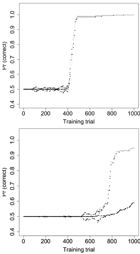
the mutation probability to 0.25, and the probabili-ties of each individual mutation type to 0.1. In 17 of them, performance on the 1000th trial was above 0.90 correct. Two examples are shown in Figure 4 to illustrate the variety of simulation behavior.

In the top panel, performance is initially at chance on all pairs. As the constraint population diversi-fies, so do the error probabilities of the individual pairs, but average performance stays at chance. That changes after two near-simultaneous innovations, the fell-swoop constraint C9 = ⇤[ voice]] (Trial

378) and a parochial versionC11=⇤V : [ voice]]

(Trial 384) that applies only when the vowel is long (tense). Both macro-constraints prosper, but greater generality ofC9gives it a reproductive advantage (it

breeds wheneverC11 does, but not vice versa). By

Trial 999,C9is represented 591 times in the

popula-tion (equivalent to a weight of591_·⇣ = 5.91). The

slight bifurcation at the end, visible as a thickening of the gray line, is due to 48 instances of C11 that

cause slightly better accuracy for long vowels. In the bottom panel, the fell-swoop constraint

⇤[ voice]] does not arise until Trial 732, by which

[image:9.612.74.304.68.485.2]

Figure 4:Probability of correct response to the specific winner-loser pair presented on each trial, for one run of the simulation. Black points show errors.

two have prospered unequally (284⇥ vs. 28⇥ on Trial 999), so that the learning curves for the two syllable types diverge. The fell-swoop constraint is still feeble (7⇥) because the learner nearly stopped making errors on long-vowel syllables before it was discovered, so its weight now grows in tandem with that of the short-vowel constraint. When the simula-tion ends the learner is near-perfect when the vowel is long, but only a bit above chance when it is short. The early discovery of a solution for a subset of the data has inhibited a more general solution.

9 Discussion

Sigmoidal abruptness in an observed learning curve has often been taken as distinguishing “rule-based” learning by serial hypothesis testing from “cue-based” associative learning by gradual weight changes (Ashby et al., 1998; Love, 2002; Maddox and Ashby, 2004; Smith et al., 2012; Kurtz et al., 2013). The theory is that while the curve is flat, the learner is serially testing and discarding incor-rect rule hypotheses, and the jump occurs when the correct rule is found. The Winnow-MaxEnt-Subtree Breeder model shows that the same obser-vation is consistent with an incremental constraint-based learner. While the curve is flat, this learner is exploring the space of possible constraints, and the jump occurs when a useful mutant arises and pros-pers.

This behavior leads to a hypothesis. Becker and Tessier (2011) have proposed a correlation between abruptness and innateness (or at least pre-existing-ness), viz., that a U-shaped kink in an L1 learning curve means that the learner has innovated a con-straint and added it at the top of the hierarchy, caus-ing a transient drop in adult-like performance. Anal-ogously, the behavior of Winnow-MaxEnt-Subtree Breeder implies that patterns which depend only on preexisting constraints (supplied by Universal Grammar, or transferred from a previously-acquired language) should be acquired less abruptly than pat-terns which depend on constraints that are specific to the particular natural or artificial language.

Another consequence is an emergent bias in favor of more-general constraints. In Winnow-MaxEnt-Subtree Breeder, general constraints automatically outcompete parochial ones because they are more fit (see discussion of Figure 4, above; Pater and More-ton 2012; MoreMore-ton et al. 2017, §4.1). In that

re-spect, the model is akin to the Minimum Description Length learner of Rasin and Katzir (2016), which adds, removes, and changes constraints without try-ing to anticipate their effects, rather than learners in which a drive towards generalization is hard-wired into the constraint-generation component (Hayes and Wilson 2008,§4.2.2, Adriaans and Kager 2010,

References

Adriaans, F. and R. Kager (2010). Adding gener-alization to statistical learning: the induction of phonotactics from continuous speech. Journal of Memory and Language 62(3), 311–331.

Ashby, F. G., L. A. Alfonso-Reese, A. U. Turken, and E. M. Waldron (1998). A neuropsychological theory of multiple systems in category learning.

Psychological Review 105(3), 442–481.

Barlow, J. A. and D. A. Dinnsen (1998). Asymmet-rical cluster development in a disordered system.

Language Acquisition 7(1), 1–49.

Becker, M. and A. Tessier (2011). Trajectories of faithfulness in child-specific phonology. Phonol-ogy 28, 163–196.

Boersma, P. and J. Pater (2016). Convergence prop-erties of a gradual learning algorithm for Har-monic Grammar. In J. J. McCarthy and J. Pater (Eds.),Harmonic Grammar and Harmonic Seri-alism, pp. 389–434. Sheffield, England: Equinox. Bradley, R. A. and M. E. Terry (1952). Rank anal-ysis of incomplete block designs: I. the method of paired comparisons. Biometrika 39(3/4), 324– 345.

Burzio, L. (1999). Surface-to-surface morphol-ogy: when your representations turn into con-straints. MS, Department of Cognitive Science, Johns Hopkins University. ROA-341.

Byrd, R. H., P. Lu, J. Nocedal, and C. Zhu (1995). A limited memory algorithm for bound constrained optimization.SIAM Journal of Scientific Comput-ing 16, 1190–1208.

Cramer, N. L. (1985). A representation for the adap-tive generation of simple sequential programs. In J. Grefenstette (Ed.),Proceedings of the First In-ternational Conference on Genetic Algorithms, pp. 183–187.

Dietrich, A. and H. Haider (2015). Human creativ-ity, evolutionary algorithms, and predictive repre-sentations: the mechanics of thought trials. Psy-chonomic Bulletin and Review 22, 897–915. Gerlach, S. R. (2010). The acquisition of

conso-nant feature sequences: harmony, metathesis, and deletion patterns in phonological development. Ph. D. thesis, University of Minnesota.

Goldwater, S. J. and M. Johnson (2003). Learning OT constraint rankings using a maximum entropy

model. In J. Spenader, A. Erkisson, and O. Dahl (Eds.), Proceedings of the Stockholm Workshop on Variation within Optimality Theory, pp. 111– 120.

Golston, C. (1996). Direct Optimality Theory: Rep-resentation as pure markedness. Language 72(4), 713–748.

Gussenhoven, C. and H. Jacobs (2005). Understand-ing phonology (2nd ed.). Understanding Lan-guage Series. London: Hodder Arnold.

Guy, G. R. (2014). Linking usage and grammar: generative phonology, exemplar theory, and vari-able rules. Lingua 142, 57–65.

Hayes, B. and C. Wilson (2008). A Maximum Entropy model of phonotactics and phonotactic learning. Linguistic Inquiry 39(3), 379–440. Ito, J. and R. A. Mester (2003). On the sources

of opacity in OT: coda processes in German. In C. F´ery and R. van de Vijver (Eds.),The syllable in Optimality Theory, pp. 271–303. Cambridge, England: Cambridge University Press.

J¨ager, G. (2007). Maximum Entropy models and Stochastic Optimality Theory. In J. Grimshaw, J. Maling, C. Manning, J. Simpson, and A. Zae-nen (Eds.),Architectures, rules, and preferences: a festschrift for Joan Bresnan, pp. 467–479. Stan-ford, California: CSLI Publications.

Koza, J. R. (1989). Hierarchical genetic algo-rithms operating on populations of computer pro-grams. InProceedings of the 11th International Joint Conference on Artificial Intelligence, Vol-ume 1, San Mateo, California, pp. 768–774. Mor-gan Kaufmann.

Kurtz, K. J., K. R. Levering, R. D. Stanton, J. Romero, and S. N. Morris (2013). Human learning of elemental category structures: revis-ing the classic result of Shepard, Hovland, and Jenkins (1961).Journal of Experimental Psychol-ogy: Learning, Memory, and Cognition 39(2), 552–572.

Legendre, G., Y. Miyata, and P. Smolensky (1990). Can connectionism contribute to syntax? Har-monic Grammar, with an application. In M. Zi-olkowski, M. Noske, and K. Deaton (Eds.), Pro-ceedings of the 26th Regional Meeting of the Chicago Linguistic Society, Chicago, pp. 237– 252. Chicago Linguistic Society.

co-occurrence constraints in L1 acquisition. Lin-guistics in the Netherlands 24(1), 162–172. Littlestone, N. (1988). Learning quickly when

ir-relevant attributes abound: a new linear-threshold algorithm. Machine Learning 2, 285–318. Love, B. C. (2002). Comparing supervised and

un-supervised category learning. Psychonomic Bul-letin and Review 9(4), 829–835.

Luce, R. D. (1977). The Choice Axiom after twenty years. Journal of Mathematical Psychology 15, 215–233.

Luce, R. D. (2005 [1959]).Individual choice behav-ior: a theoretical analysis. New York: Dover. Macken, M. A. and D. Barton (1978, March). The

acquisition of the voicing contrast in English: a study of voice-onset time in word-initial stop con-sonants. Report from the Stanford Child Phonol-ogy Project.

Macmillan, N. A. and C. D. Creelman (2004). De-tection Theory: A User’s Guide. Cambridge, Eng-land: Lawrence Erlbaum.

Maddox, W. T. and F. G. Ashby (2004). Dissociating explicit and procedural-learning based systems of perceptual category learning. Behavioural Pro-cesses 66, 309–332.

Magri, G. (2013). HG has no computational advan-tages over OT: toward a new toolkit for computa-tional OT. Linguistic Inquiry 44(4), 569–609. McCarthy, J. J. (1999). Introductory OT on

CD-ROM. Graduate Linguistic Students’ Association, University of Massachusetts, Amherst.

Mitrinovi´c, D. S. (1970).Analytic inequalities. New York: Springer-Verlag.

Moreton, E. (2010a, April). Connecting paradig-matic and syntagparadig-matic simplicity bias in phono-tactic learning. Department colloquium, Depart-ment of Linguistics, MIT.

Moreton, E. (2010b, February). Constraint induc-tion and simplicity bias. Talk given at the Work-shop on Computational Modelling of Sound Pat-tern Acquisition, University of Alberta.

Moreton, E. (2010c, May). Constraint induction and simplicity bias in phonotactic learning. Handout from a talk at the Workshop on Grammar Induc-tion, Cornell University.

Moreton, E. (2018). Conditions on abruptness in a gradient-ascent Maximum Entropy learner. In G. Jarosz and J. Pater (Eds.), Proceedings of the

Society for Computation in Linguistics, Volume 1, pp. Article 13.

Moreton, E., J. Pater, and K. Pertsova (2017). Phonological concept learning. Cognitive Sci-ence 41(1), 4–69.

Moreton, E. and K. Pertsova (2016). Implicit and explicit processes in phonotactic learning. In TBA (Ed.),Proceedings of the 40th Boston Uni-versity Conference on Language Development, Somerville, Mass., pp. TBA. Cascadilla.

Nakano, K., H. Hiraki, and S. Ikeda (1995). A learning machine that evolves. InProceedings of ICEC–95, pp. 808–813.

Novikoff, A. B. (1963). On convergence proofs for perceptrons. Technical report, Stanford Research Institute.

Pater, J. (2004). Austronesian nasal substitution and other⇤N C effects. In J. J. McCarthy (Ed.), Op-timality Theory in phonology: a reader, Chap-ter 14, pp. 271–289. Malden, Mass.: Blackwell. Pater, J. and E. Moreton (2012). Structurally

bi-ased phonology: complexity in learning and ty-pology. Journal of the English and Foreign Lan-guages University, Hyderabad 3(2), 1–44. Pizzo, P. (2013, January 19). Learning

phonologi-cal alternations with online constraint induction. Slides from a presentation at the 10th Old World Conference on Phonology (OCP 10).

Prince, A. and P. Smolensky (1993).Optimality The-ory: constraint interaction in generative gram-mar. Department of Linguistics, Rutgers Univer-sity.

R Core Team (2015). R: A Language and Environ-ment for Statistical Computing. Vienna, Austria: R Foundation for Statistical Computing.

Rasin, E. and R. Katzir (2016). On evaluation met-rics in optimality theory.Linguistic Inquiry 47(2), 235–282.

Rosenblatt, F. (1958). The perceptron: a probabilis-tic model for information storage and organiza-tion in the brain. Psychological Review 65(6), 386–408.

Saffran, J. R. and E. D. Thiessen (2003). Pattern induction by infant language learners. Develop-mental Psychology 39(3), 484–494.

328.

Simonton, D. K. (2004). Creativity in science: chance, logic, genius, and Zeitgeist. Cambridge University Press.

Smith, J. D., M. E. Berg, R. G. Cook, M. S. Murphy, M. J. Crossley, J. Boomer, B. Spiering, M. J. Be-ran, B. A. Church, F. G. Ashby, and R. C. Grace (2012). Implicit and explicit categorization: a tale of four species. Neuroscience and Biobehavioral Reviews 36(10), 2355–2369.

Smith, J. L. (2003). Onset sonority constraints and subsyllabic structure. MS, Department of Lin-guistics, University of North Carolina, Chapel Hill. ROA-602.

Smith, J. L. (2012). The formal definition of the ON -SET constraint and implications for Korean

syl-lable structure. In T. Borowsky, S. Kawahara, T. Shinya, and M. Sugahara (Eds.),Prosody mat-ters: essays in honor of Elisabeth Selkirk, pp. 73– 108. Equinox.

Smith, N. V. (1973). The acquisition of phonology: a case study. Cambridge, England: Cambridge University Press.

Strauss, D. (1992). The many faces of logistic re-gression. American Statistician 46(4), 321–327. Sutton, R. S. and A. G. Barto (1981). Toward a