Efficient Learning of Output Tier-Based Strictly 2-Local Functions
Phillip Burness University of Ottawa [email protected]
Kevin McMullin University of Ottawa
Abstract
This paper characterizes the Output Tier-based Strictly k-Local (OTSLk) class of string-to-string functions, which are relevant for mod-eling long-distance phonological processes as input-output maps. After showing that any OTSLkfunction can be learned whenkand the tier are given, we present a new algorithm that induces the tier itself whenk= 2and provably learns any total OTSL2function in polynomial time and data—the first such learner for any class of tier-based functions.
1 Introduction
In this paper, we investigate the class of Output Tier-based Strictlyk-Local (OTSLk) functions. In
terms of finite state transducers, OTSLkfunctions
are those for which the output symbol(s) to be written at each timestep depends on thek−1most recent symbols on the output tape that belong to the relevant ‘tier’ (a subset of the output alphabet; Heinz et al., 2011), without regard for any non-tier symbols that might have been written between them or after them. We show that they are learn-able when the contents of the tier are provided as input to the learner, and introduce an algorithm that provably and efficiently learns any total OTSL function whenk= 2.
Recent research investigating the computational properties of phonological patterns observed in natural language has shown that many attested processes can be characterized as Strictly Local (SL) functions (Chandlee,2014;Chandlee et al., 2014, 2015). That is, the output at any given timestep is dependent on the previousk−1 sym-bols from either the input string (Input Strictlyk -Local; ISLk) or the output string (Output Strictly k-Local; OSLk). Multiple characterizations of
these classes exist and their properties are well-understood. One important distinction between
the two is that non-iterative processes are ISL, whereas processes that apply iteratively to multi-ple targets are OSL. Moreover, efficient learning algorithms exist for both the ISL and OSL func-tions. The OSL Function Inference Algorithm (OSLFIA; Chandlee et al., 2015) is of particular importance to this paper, as we will show that many of their theoretical results can be general-ized to OTSL functions in a natural way.
Long-distance phonological processes, for which a potentially unbounded number of seg-ments may intervene between the trigger and tar-get without being affected in any way, are nei-ther ISL nor OSL for any value of k. For exam-ple, Samala has a long-distance process of sibi-lant harmony in which an underlying /s/ surfaces as [S] if another [S] appears anywhere later in the word. This is seen when, e.g., the perfective suffix /-waS/ is added to a root containing /s/, as in /ha-s-xintila-waS/→[haSxintilawaS] ‘his former gentile name’ (Applegate,1972). This process can be un-derstood as applying iteratively to multiple targets, as in /s-lu-sisin-waS/→[SluSiSinwaS] ‘It is all grown awry’. Indeed, it seems that the vast majority of attested long-distance processes are enforced iter-atively (Kaplan,2008;Hansson,2010). As such, we focus this paper on OTSLkfunctions in
partic-ular, which generalize the OSLkclass in a way that
allows us to model these kinds of long-distance processes. We note that ITSLk functions can be
characterized in a similar way and that the learning strategy outlined below could likely be extended to total ITSL2functions.
While the notion of a tier has long been incor-porated into phonological theory (e.g.,Clements, 1980;Goldsmith,1990;Odden,1994;Heinz et al., 2011;McMullin,2016), the range of possible tiers is typically assumed to be available to the learner
natural classes of segments (e.g.,Hayes and Wil-son, 2008). Though algorithms have been de-veloped for inducing a relevant tier from a sam-ple of positive training, their success is limited to phonotactic co-occurrence restrictions. This is true both for constraint-based maximum en-tropy learners (Gouskova and Gallagher,2019) as well as for algorithms that learn grammars for Tier-based Strictly Local formal languages (Jar-dine and Heinz, 2016; Jardine and McMullin, 2017). To our knowledge, the algorithm pre-sented below, which we call the Output Tier-based Strictly 2-Local Function Inference Algorithm (OTSL2FIA), is the first algorithm which learns the relevant tier for transformations of underlying representations (strings of input segments) to sur-face forms (strings of output segments).
The remainder of this paper is organized as fol-lows. Notation and relevant concepts are pre-sented in Section 2. In Section 3, we define the OTSL functions and characterize them in terms of finite state transducers. In Section4, we high-light several important properties of OTSL2
func-tions in particular that can be taken advantage of during learning. All aspects of the learning algo-rithm, along with the theoretical learning results, are described in Section 5. Section 6 discusses how OTSL2 functions can model various
phono-logical processes and identifies several avenues for future research. Section7concludes.
2 Preliminaries 2.1 Strings and sets
Given a setS, we writecard(S)to denote its car-dinality. For a string w made of symbols from some alphabet Σ, |w| denotes the length of the string. We writeΣ∗ to denote all possible strings made from the alphabetΣ, whileΣn denotes all possible strings made from that alphabet with a length ofn, andΣ≤ndenotes all such strings with a length up ton. The unique string of length 0 (the empty string) is written asλ. Given two stringsu
andv, we writeu·vto denote their concatenation, but often shorten this touvwhen context permits. We write fack(w) to denote all the contiguous substrings of lengthk(thek-factors) contained in a stringw.
We assume a fixed but arbitrary total order ≺ over the letters of Σ, an order which we ex-tend to all strings in Σ∗ by defining the length-lexicographical order(Oncina et al.,1993;
Chan-dlee et al., 2015) as follows. String w1
oc-curs length-lexicographically before w2 (written
as w1 / w2) when |w1| < |w2| or, if |w1| =
|w2|, when ai ≺ bi where ai is the ith letter in w1, bi is the ith letter in w2, and i is the first
position on which w1 andw2 differ. For
exam-ple, given Σ = {a, b} where a ≺ b, we have
λ / a / b / aa / ab / ba / bb / aaaand so on. A prefix of some string wis any string usuch thatw = uxandx ∈ Σ∗. Similarly, a suffix of some stringwis any stringusuch thatw=xuand
x∈Σ∗. Note that any string is a prefix and suffix of itself, and thatλis a prefix and suffix of every string. When|w| ≥n,Prefn(w)andSuffn(w)
denote the unique prefix and suffix of w with a length ofn; when|w|< n, they simply denotew
itself. We writePref∗(w)to denote the set of all prefixes of w. Also, Suffn(Suffn(w1)w2)) =
Suffn(w1w2). Given a string w, one of its
pre-fixesp, and one of its prefixess, we writep−1·w
to represent the stringwwithout that prefixpand write w· s−1 to represent the string w without that suffix s. For example, a−1 ·aba = ba and
aba·a−1 = ab. Finally, given a set of stringsS, we write lcp(S) to denote the longest common prefixofS, which is the stringu such thatu is a prefix of every w ∈ S, and there exists no other stringvsuch that|v|>|u|andvis also a prefix of everyw∈S.
2.2 Functions and transducers
This paper deals exclusively with string-to-string functions, relations that pair everyw∈Σ∗with at most oney∈∆∗, whereΣand∆are the input al-phabet and output alal-phabet respectively. The input language and output language of such a function are pre image(f) = {x |(∃y)[x 7→f y]} and
image(f) = {y |(∃x)[x 7→f y]}, respectively. An important concept is that of thetailsof an in-put stringwwith respect to a functionf.
Definition 1. (Tails) Given a function f and an inputw ∈ Σ∗,tailsf(w) ={(y, v)|f(wy) = uv∧u=lcp(f(wΣ∗))}.
In words, tailsf(w) pairs every possible string y ∈ Σ∗ with the portion of f(wy) that is directly attributable toy. That is, it describes the effect thatwhas on the output of any subsequent string of input symbols. When tailsf(w1) =
tailsf(w2) we say that w1 and w2 are
tail-equivalentwith respect tof.
is thecontributionof a symbola∈Σrelative to a stringw∈Σ∗ with respect to a functionf.
Definition 2. (Contribution)Given a function f, somea ∈ Σ, and somew ∈ Σ∗, contf(a, w) = lcp(f(wΣ∗))−1·lcp(f(waΣ∗)).
In words, for an input stringx that has the prefix
wa, the contribution of theainwais the portion off(x)that is uniquely and directly attributable to that instance ofa.
The Output Tier-based Strictly Local functions that will be introduced below are a proper subclass of the subsequential functions.Oncina and Garc´ıa (1991) show that when a function is subsequen-tial, tail-equivalency will partitionΣ∗into finitely many blocks, allowing us to construct a finite-state transducer that computesf. In this paper we use delimited subsequential finite state transducers (DSFSTs; see Jardine et al., 2014), to character-ize the class of Output Strictly Local (OSL) func-tions. The following definition is drawn directly fromChandlee et al.(2015).
Definition 3. A delimited subsequential fi-nite state trasnducer (DSFST) is a 6-tuple
hQ, q0, qf,Σ,∆, δiwhereQis a finite set of states, q0 ∈ Q is the unique initial state, qf ∈ Q is
the unique final state, Σ is the finite input al-phabet, ∆is the finite output alphabet, andδ ⊆
Q×(Σ∪ {o,n})×∆∗×Qis the transition
func-tion (whereo∈/ Σindicates the start of the input andn∈/Σindicates the end of the input), and the
following hold:
1. if(q, a, u, q0)∈δthenq=6 qf andq06=q0
2. if(q, a, u, qf)∈δthena=nandq6=q0
3. if (q0, a, u, q0) ∈ δ then a = o and if (q,o, u, q0)∈δthenq=q0
4. if(q, a, u, q0),(q, a, u0, q00) ∈δ thenq0 = q00
andu=u0
Each transition (q, a, u, q0) ∈ δ can be seen as an instruction to append u to the end of the output tape and to move to state q0 upon read-ing a while in state q. This transition func-tion may be partial, and its recursive exten-sion δ∗ is the smallest set containing δ closed under the following conditions: (q, λ, λ, q) ∈
δ∗, and (q, w, u, q0),(q0, a, v, q00) ∈ δ∗ ⇒
(q, wa, uv, q00) ∈ δ∗. The initial state of a DS-FST has no incoming transitions and has exactly
one outgoing transition, which will be for the in-putoand does not land in the final state.
Further-more, the final state of a DSFST has no outgoing transitions, and every transition into the final state is for the inputn. DSFSTs are also deterministic
on the input, such that each state has at most one outgoing transition per input symbol.
The size of a DSFSTT = hQ, q0, qf,Σ,∆, δi
is|T |=card(Q) +card(δ) +P
(q,a,u,q0)∈δ|u|,
and the relation defined by a DSFST isR(T) =
{(x, y)∈Σ∗×∆∗|(q0,oxn, y, qf)∈δ∗}.
The DSFSTs we will use below have a special property known asonwardness, which informally means that the writing of the output is never de-layed. The following formal definition of onward-ness and a related lemma are borrowed from Chan-dlee et al.(2015).
Definition 4. (Onwardness)A DSFST isonwardif for every w ∈ Σ∗ andu ∈ ∆∗, (q0,ow, u, q) ∈ δ∗⇐⇒u=lcp(f(wΣ∗)).
Lemma 1. Let the outputs of the edges out of state q be Outputs(q) = {u | (∃a ∈
Σ ∪ {o,n}) (∃q0 ∈ Q) [(q, a, u, q0) ∈ δ]}.
If T is an onward DSFST and recognizes f,
then ∀q 6= q0, lcp(Outputs(q)) = λ and
lcp(Outputs(q0)) =lcp(f(Σ∗)).
Below we will frequently make reference to the length-lexicographically earliest input string that can lead to a stateqin a given transducerT, which we will denote aswq. A formal definition is pro-vided here for reference.
Definition 5. (Earliest string)Given a transducer
T = hQ, q0, qf,Σ,∆, δi, the earliest string that
leads to q ∈ Q is wq = min/{w ∈ Σ∗ | ∃u,(q0,ow, u, q)∈δ∗}.
A distinction that will be important throughout the rest of this paper is that between the writing that occurs in a DSFST as it is reading letters from Σ, and the writing that occurs at the very end (when the DSFST readsn). To make this
dis-tinction,Chandlee et al.(2015) defined the prefix functionfp associated with a subsequential func-tionf as follows.
Definition 6. (Prefix function) Given a subse-quential function f, its associated prefix function
fpis such thatfp(w) =lcp(f(wΣ∗)).
Remark 1. Given a subsequential function f, some a ∈ Σ, and some input string w ∈
2.3 Strict locality and tiers
Chandlee(2014) andChandlee et al.(2014) orig-inally introduced the Input Strictly Local (ISL) and Output Strictly Local (OSL) functions, both of which generalize Strictly Local (SL) stringsets to functions based on one of the defining proper-ties of SL languages, the Suffix Substitution Clo-sure (Rogers and Pullum, 2011). The definitions of the ISL and OSL functions exploit a corollary of this defining property, which Chandlee et al. (2015) call Suffix-defined Residuals. For reasons of space, we only discuss the OSL functions be-low.
Theorem 1. (Suffix Substitution Closure) A lan-guageLis SL if for all stringsu1, v1, u2, v2there
exists a natural numberksuch that for any string
x of length k − 1, if u1xv1, u2xv2 ∈ L, then u1xv2∈L.
Corollary 1. (Suffix-defined Residuals) A lan-guage L is SL if for all w1, w2 ∈ Σ∗, there
ex-ists a natural numberksuch that ifSuffk−1(w1) = Suffk−1(w2) then {v | w1v ∈ L} = {v | w2v∈L}, that isw1andw2 have the same
resid-uals(tails) with respect toL.
Definition 7. (Output Strictly Local functions)
A function f is OSLk if for all w1, w2 ∈ Σ∗, Suffk−1(fp(w1)) = Suffk−1(fp(w2)) ⇒
tailsf(w1) =tailsf(w2).
Chandlee (2014) and Chandlee et al. (2014, 2015) show that most iterative phonological pro-cesses can be modelled with an OSL function, with an important exception being long-distance iterative processes like consonant harmony. This is parallel to the fact that long-distance phonotac-tics cannot be represented with an SL stringset, which motivated Heinz et al. (2011) to define the Tier-based Strictly Local (TSL) languages— stringsets that are SL after an erasure function has applied, masking all symbols that are irrelevant to the restrictions that the language places on its strings.
Definition 8. (Erasure function)Given an alpha-betΣ, a tier Θ ⊆ Σ, and a stringw = a1...an,
EraseΘ(w) = b1...bn where for all i ≤ n, bi =aiifai∈Θ, elsebi =λ.
Informally, EraseΘ(w) returns the string w
with all non-tier elements removed. For con-venience, we will write SuffnΘ(w) to mean Suffn(EraseΘ(w))in what follows.
Definition 9. (Tier-based Strictly Local lan-guages) A language L is Tier-based Strictly k -Local (TSLk) if there is a tierΘ⊆Σand a subset
S⊆fack(oΘ∗n)such that:
L={w∈Σ∗ |fack(oEraseΘ(w)n)⊆S}
3 Output Tier-based Strictly Local functions and transducers
In this section, we define the OTSL functions, which generalize the TSL stringsets to functions in the same way that the OSL functions general-ize SL stringsets to functions (seeChandlee,2014; Chandlee et al.,2015).
Definition 10. (Output Tier-based Strictly Lo-cal functions) A function f is OTSLk if there
is a tier Θ ⊆ ∆ such that for all w1, w2 ∈ Σ∗, SuffkΘ−1(fp(w1)) = SuffkΘ−1(fp(w2)) ⇒
tailsf(w1) =tailsf(w2).
The OTSL class properly contains the OSL functions, since every OSLk function can be
de-scribed as an OTSLkfunction whose tier is equal
to the entire output alphabet. Note that it is pos-sible for a single OTSL function to be described with more than one tier. For example, the identity function (whereΣ = ∆andf(w) = w) can be described with any subset of∆as its tier. We use the termk-tier to describe a tierΘfor whichf is OTSLk.
Like the OSLkfunctions, the OTSLkfunctions
can be characterized in automata-theoretic terms. First, we define OTSLk finite state transducers as
follows.
Definition 11. An onward DSFST T =
hQ, q0, qf,Σ,∆, δiis OTSLk for the tier Θ ⊆ ∆
if:
1. Q=S∪ {q0, qf}withS ⊆Θ≤k−1
2. (∀u∈∆∗)
[(q0,o, u, q0)∈δ ⇒q0=SuffkΘ−1(u)]
3. (∀q ∈Q− {q0},∀a∈Σ,∀u∈∆∗) [(q, a, u, q0)∈δ⇒q0 =SuffkΘ−1(qu)].
Lemmas 2 and 3, together with Theorem 2, show that the OTSLk functions and the functions
represented by OTSLk transducers exactly
corre-spond.
Lemma 2. Let T = hQ, q0, qf,Σ,∆, δi be an
OTSLk transducer for the tier Θ. The following
Lemma 3. Any OTSLktransducer corresponds to
an OTSLkfunction.
Theorem 2. Given an OTSLk function f and one of its k-tiers Θ, the DSFST T =
hQ, q0, qf,Σ,∆, δidefined as follows computesf:
1. Q=S∪ {q0, qf}withS⊆Θ≤k−1
2. (q0,o, u,SuffΘk−1(u))∈δ⇐⇒u=fp(λ)
3. a∈Σ,(q, a, u,Suff1Θ(qu))∈δ⇐⇒
(∃w) [fp(w) =vr∧SuffkΘ−1(vr) =q∧
fp(wa) =vru]
wherer=t1x1t2x2...tk−1xk−1,
ti∈Θ, xi ∈(∆−Θ)∗andv=fp(w)·r−1
4. (q,n, u, qf)∈δ⇐⇒u=fp(wq)−1·f(wq)
We note that these are trivial extensions of Lem-mas 3, 4, and Theorem 2 in Chandlee et al. (2015). Indeed, only two minor changes are necessary for this generalization to OTSLk
func-tions. First, each instance of Suffk−1 must be replaced with SuffkΘ−1. Second, in order to ac-count for the fact that non-tier elements may come between relevant tier elements, certain references to a string q = t1t2...tk−1 must be rewritten as r = t1x1t2x2...tk−1xk−1, where ti ∈ Θ and xi ∈(∆−Θ)∗. As the proofs are otherwise
iden-tical in structure to those found inChandlee et al. (2015), we do not provide them here.
It is therefore the case that any OTSLkfunction
can be represented by an OTSLktransducer.
Infor-mally, this will be an onward DSFST in which the non-initial and non-final states represent the most recentk−1tier symbols written thus far, meaning that this is the only information that will dictate what the DSFST writes upon reading the next in-put symbol.
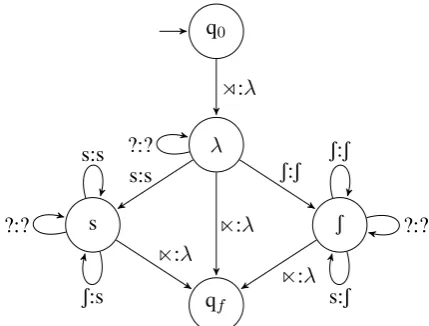
As an example, Figure 1 presents an OTSL2
transducer that models the unbounded sibilant har-mony in Samala from Section1. Note that in order to achieve the regressive directionality of the pro-cess, we assume that this transducer reads input strings from right-to-left (following, e.g., Heinz and Lai,2013;Chandlee et al.,2015). Direction-ality will be further discussed in Section6.
4 Useful properties of OTSL2functions
The main goal of this paper is to demonstrate how OTSL functions can be learned from positive data, even without prior knowledge of the tier itself. We note that the tier-induction strategy adopted below
q0
λ
S s
qf o:λ
?:?
S:S s:s
S:S
s:S
?:? s:s
S:s
?:? n:λ
n:λ
[image:5.595.308.523.61.224.2]n:λ
Figure 1: An OTSL2 transducer that models un-bounded sibilant harmony, where ? represents any symbol that is not s orS
relies on certain properties that hold whenk= 2, but not necessarily for greater values ofk. These are outlined below.
First, when an OTSL2 function f can be
de-scribed with more than one2-tier, the union of any two or more such2-tiers is also a2-tier forf.
Lemma 4. Given an OTSL2functionf, ifΘ1⊆∆
and Θ2 ⊆ ∆ are both 2-tiers for f, then Ω = Θ1∪Θ2is also a2-tier forf.
Proof. IfSuff1Ω(fp(w1)) = Suff1Ω(fp(w2)) = t, then t ∈ Θ1 or t ∈ Θ2. If t ∈ Θ1,
then Suff1Θ 1(f
p(w
1)) = Suff1Θ1(f
p(w 2)) = t ⇒ tailsf(w1) = tailsf(w2). If t ∈ Θ2, then Suff1Θ2(fp(w1)) = Suff1Θ2(fp(w2)) = t ⇒ tailsf(w1) = tailsf(w2).
There-fore,Suff1Ω(fp(w1)) =Suff1Ω(fp(w2)) =t⇒
tailsf(w1) =tailsf(w2)
It is this property that allows us to identify a uniquetarget tier for an OTSL2 function, which
the algorithm can find by flagging and removing elements of∆from its hypothesis when evidence is found that they cannot be on a relevant tier. We define this canonical2-tier as follows.
Definition 12. (Canonical2-tier)Given an OTSL2
function f, Θ is the canonical 2-tier for f iff there is no other 2-tier Ω ⊆ ∆ for f such that
card(Ω)≥card(Θ).
Remark 2. Given an OTSL2functionf, its
canon-ical2-tierΘis a superset of any2-tier forf. (This follows immediately from Lemma4.)
There is therefore a unique canonical 2-tier (i.e., the largest one) for each OTSL2 function.
process, since it leads to the following useful prop-erty of OTSL2functions.
Lemma 5. Letf : Σ∗ → ∆∗ be an OTSL2
func-tion, let Θ be its canonical 2-tier, and let Ω be such thatΘ ⊂Ω ⊆ ∆. We have∃a ∈ (Ω−Θ),
∃w1, w2 ∈ Σ∗, and ∃x ∈ Σ ∪ {n} such that Suff1Ω(fp(w1)) = Suff1Ω(fp(w2)) = a and contf(x, w1)6=contf(x, w2).
Proof. By contradiction. Suppose that the lemma is false. This means that∀a∈(Ω−Θ),∀w1, w2∈ Σ∗, and∀x∈Σ∪ {n}, we haveSuff1Ω(fp(w1)) = Suff1Ω(fp(w
2)) = a ⇒ contf(x, w1) =
contf(x, w2). Now, since Θ is a 2-tier for f,
it is also the case that ∀b ∈ Θ, ∀w1, w2 ∈ Σ∗,
and ∀x ∈ Σ ∪ {n}, we have Suff1Ω(fp(w 1)) = Suff1Ω(fp(w2)) = b ⇒ contf(x, w1) =
contf(x, w2). Together these imply that ∀c ∈ Ω, ∀w1, w2 ∈ Σ∗, and ∀x ∈ Σ ∪ {n}, we
haveSuff1Ω(fp(w1)) =Suff1Ω(fp(w2)) =c⇒
contf(x, w1) =contf(x, w2).
Since [Suff1Ω(fp(w1)) = Suff1Ω(fp(w2))
and contf(x, w1) = contf(x, w2)] ⇒
Suff1Ω(fp(w
1x)) = Suff1Ω(fp(w2x)), we
also have contf(y, w1x) = contf(y, w2x)
for all y ∈ Σ ∪ {n}. This applies recursively, giving us Suff1Ω(fp(w
1)) = Suff1Ω(fp(w2))
⇒ tailsf(w1) = tailsf(w2), which means
that Ω is a 2-tier for f. However, card(Ω) >
card(Θ), contradicting the fact that Θ is the canonical2-tier forf.
Importantly, it follows from Lemma5 that for any set Ω which is a strict superset of Θ (the canonical 2-tier), we will always be able to find evidence that some member of Ωcould not be a member of any 2-tier for f. It is this property of OTSL2 functions that our algorithm makes use
of to determine which output symbols are in Θ. Once again, whenk > 2, this property does not necessarily hold.1 Accordingly, we restrict our-selves to k = 2 when discussing the learning of OTSL functions without prior knowledge of the tier. While OTSL2 functions seem sufficient for
modelling a wide range of long-distance phono-logical processes, we discuss certain exceptions in Section6.
1For example, if∆ ={a, b, c}, there could be an OTSL
3
function for whichΘ1 ={a, b}andΘ2 ={a, c}are both
3-tiers, butΩ ={a, b, c}is not.
5 Learning OTSL functions 5.1 Learning paradigm
We adopt the criterion for successful learning that requires exact identification in the limit from pos-itive data (Gold, 1967), with polynomial bounds on time and data (de la Higuera, 1997). We first define what it means for a class of functions to be represented by a class of representations.
Definition 13. A class T of functions is repre-sented by a classRof representations if everyr∈ Ris of finite size and there is a total and surjective
naming functionL:R→ Tsuch thatL(r) =tif
and only if for allw ∈ pre image(t), r(w) = t(w), where r(w) is the output produced by r
given the inputw.
The notions of a sample and a learning algo-rithm are defined as follows.
Definition 14. (Sample)A sampleSfor a function
t ∈Tis a finite set of data consistent witht, that is to say(w, u) ∈ S iff t(w) = v. The size of a sample is the sum of the length of the strings it is composed of:|S|=P
(w,u)∈S|w|+|u|.
Definition 15. (Learning algorithm) A (T,R)
-learning algorithm Ais a program that takes as input a sample for a functiont∈Tand outputs a representation fromR.
The paradigm relies on the notion of a charac-teristic sample, adapted here for functions as in Chandlee et al.(2015).
Definition 16. (Characteristic sample) For a
(T,R)-learning algorithm A, a sample CS is a
characteristic sample of a function t ∈ T if for all samplesS⊇CS,Areturns a representationr
such thatL(r) =t.
The learning paradigm can now be defined as follows.
Definition 17. (Identification in polynomial time and data)A classTof functions is identifiable in polynomial time and data if there exists a(T,R)
-learning algorithm A and two polynomial equa-tionsp()andq()such that:
1. For any sample S of size m for t ∈ T, A
returns a hypothesisr∈RinO(p(m))time.
5.2 Learning when the tier is given
Prior to describing the approach we take to induc-ing the contents of a tier whenk= 2, we note that learning any OTSLk function from positive data
is relatively straightforward if the value ofk and the tierΘare known beforehand. In particular, al-though the OSLFIA presented in Chandlee et al. (2015) was designed only to learn OSL functions, it turns out that a minor modification allows us to extend their result to OTSL functions, so long ask
andΘare known beforehand. We summarize how this can be done below.
In its original form, the OSLFIA inevitably fails to learn any OTSL function that is not itself OSL (i.e., where Θ 6= ∆). Specifically, since the al-gorithm labels each landing state of a transition with the k −1 suffix of its associated output, it will always incorrectly determine the landing state of one of more transitions when there is a long-distance dependency. Moreover, the exact way in which the resulting OSL transducer differs from the target OTSL transducer is somewhat unpre-dictable. As such, there does not seem to be a general approach for transforming the OSLFIA’s output into an appropriate OTSLktransducer.
In cases where Θ is known beforehand, how-ever, we can circumvent this issue by simply spec-ifying that non-tier elements should be skipped over when labelling a state. In doing so, the algo-rithm will be able to find all of the necessary states as well as the correct landing state for each tran-sition in the target OTSLktransducer. This
mod-ification of the OSLFIA is incorporated into the functionbuild fst, which is detailed in Algo-rithm 1. While this constitutes one important as-pect of learning OTSLkfunctions, it is nonetheless
a major challenge to determine the actual contents ofΘwithouta prioriknowledge. Although induc-ing ak-tier for any value ofkremains as an open problem, in the following section we describe how his can be done whenk= 2.
5.3 Learning the contents of a 2-tier
Having shown that the OSLFIA can be modified to learn an OTSLk functionf onceΘ(the tier) is
known, we now describe our approach to inducing
Θitself whenk= 2. After this is done,Θcan sim-ply be fed into thebuild fstfunction in order to produce an OTSL2transducer that representsf.
The first step toward learning the contents of a 2-tier is to gain as much information as possible
Functionbuild fst(S,Θ,k):
C ← {q0, qf}withq0, qf ∈/ Θ≤k−1; s←lcp({y|(x, y)∈S});
q ←SuffkΘ−1(s); Earliest(q)←o; Out(q)←s;
δ ← {(q0,o, s, q)}; R ← {q};
whileR6=∅do
q←First(R);
s←Earliest(q);
foralla∈Σin alphabetical orderdo if∃(w, u)∈S, x∈Σ∗s.t.
w=saxthen
v←lcp({y|∃x,(sax, y)∈
S});
r←SuffkΘ−1(v);
δ←
δ∪ {(q, a,Out(q)−1·v, r)};
ifr /∈R∪Cthen
R←R∪ {r}; Earliest(r)←sa; Out(r)←v;
if∃us.t.(s, u)∈Sthen
δ←δ∪{(q,n,Out(q)−1·u, qf)} R←R− {q};
C←C∪ {q}; returnhC, q0, qf,Σ,∆, δi
Algorithm 1: Building an OTSLk transducer
when givenΘ
about the prefix function fp corresponding to f, based only on the evidence provided in the training sample. To do this, the functionestimate fp, shown in Algorithm 2, goes through every string
x that is the prefix of at least one input string in the training data, and for everya ∈ Σ, it checks whetherxa is also a prefix of some input string. If this is the case, there is enough information to determine fp(x). The function estimate fp will then add the pair (x, z) to the setP, where
z is the longest common prefix of f(w) for all
(w, f(w)) ∈ S such that x is a prefix ofw. We note that this z will be equal to fp(x) provided
that the training data come from a subsequential function, and so this technique may be useful for learning other types of functions as well.
Functionestimate fp(S):
P ← ∅;
X← {x|x∈Pref∗(w), where
(w, u)∈S};
Y ← {x∈X|(∀a∈Σ)[xa∈X]}; foreachy∈Y do
z←lcp({u|(w, u)∈S, where
y∈Pref∗(w)});
P ←P∪ {(y, z)} returnP;
Algorithm 2:Prefix function estimation
This is because, when there is no pair with the shape (opaxn, f(pax))in the training data,
estimate fpdoes not know whether this is ac-cidental (i.e., due to the finite nature of the training data) or because the function is undefined for all inputs of the shapeopaxn. While the ability to
accommodate partial functions would have practi-cal applications for learning from natural language data, at present we leave the task of extending estimate fpin this way to future research.
The full learning algorithm, which we call the OTSL2 Function Inference Algorithm
(OTSL2FIA) is shown in Algorithm 3. We assume thatΣand∆are fixed and not part of the input to the learning problem (and that k = 2). Given a finite sample of training data, it first estimates the relevant prefix function with the set
P, as described above, and begins with the hy-pothesis thatΘ = ∆(i.e., that all members of the output alphabet are on the target tier). Then, for eacha ∈ Θ, it looks throughP for any evidence thata needs to be removed from Θ. To do this, it builds an auxiliary set Match that contains every(p, fp) ∈ P for whichSuff1Θ(fp(p)) = a
under the current hypothesis for Θ. For each
x∈Σ∪ {n}, it then checks whethercontf(x, p)
is the same for all(p, q) ∈ Match. If this is the case,ais added to the setKeep. However, if there is more than one value found for the contribution of some x ∈ Σ∪ {n}, it will instead remove a
fromΘ, since it cannot possibly be a member of the target 2-tier. If at any point some symbol gets removed from Θ, the set Keep is immediately emptied. This portion of the algorithm will run until everyain the current hypothesis forΘgets added to the set Keep, in which case it knows it has found the canonical 2-tier of the target function.
Once the OTSL2FIA converges on the
canon-Data:SampleS⊂ {o}Σ∗{n} ×∆∗
Result:An OTSL2transducer
T =hC, q0, qf,Σ,∆, δi P ←estimate fp(S);
Θ←∆; Keep← ∅;
whileKeep6= Θdo foreacha∈Θdo
Match← {(p, q)∈P | Suff1Θ(q) =a}; foreachσ∈Σdo
Cσ,a ← {q−1·y|
(p, q)∈Match∧(pσ, y)∈P}; ifcard(Cσ,a)>1then
Θ←Θ− {a}; Keep← ∅;
Cn,a← {q−1·y|
(p, q)∈Match∧(p, y)∈S}; ifcard(Cn,a)>1then
Θ←Θ− {a}; Keep← ∅; ifa∈Θthen
Keep←Keep∪ {a} T ←build fst(S,Θ, 2); returnT
Algorithm 3:OTSL2FIA
ical 2-tier Θ, the final step is simply to feed Θ
and the sample S into the function build fst shown above in Algorithm 1 (further specifying thatk = 2). Under the assumption that the train-ing sample contains the appropriate evidence, as described in the following section, this will pro-duce an OTSL2 transducer which represents the
target OTSL2function.
5.4 Theoretical results
Here we establish several theoretical results, which culminate in the theorem that the OTSL2FIA identifies the class of total OTSL2
functions in polynomial time and data.
In what follows, we let f be the target OTSL2
function, Θ be its canonical 2-tier, and T = hQ, q0, qf,Σ,∆, δi be its target transducer as defined by Theorem2. We furthermore let Θbe the OTSL2FIA’s final tier hypothesis, and T =
hQ, q0, qf,Σ,∆, δi be the transducer that is
con-structed on the input.
Proof. Let n = P
(w,u)∈S|w|, m = max{|u| : (w, u) ∈ S}, p = max{|w| : (w, u) ∈ S}, and
s=card(S). We note that these are all linear in the size of the sample.
The OTSL2FIA starts by calling estimate fp. This function first deter-mines all of the input prefixes present in S, which takes n steps. Then estimate fp checks, for each prefixx and alla ∈ Σ, whether
xa is also an input prefix in S. There are at most sm prefixes in S, so this takes at most card(Σ)·(sm)nsteps. Finally, for a subset of the input prefixes, estimate fp determines lcp({u | (w, u) s.t. x ∈ Pref∗(w)}), which with an appropriate data structure (for instance a prefix tree) can be done innmsteps. The overall computation time of estimate fp is thus O(n+ (sm)n+ (sm)(nm)), which is quartic in the size of the learning sample.
The portion of the OTSL2FIA that determines the tier is now run. Afterielements have been re-moved from Θ, the combinedwhile/for loop can run up to|∆| −itimes, and can only remove up to|∆|items, so the loop will be used fewer than |∆|2 times, which is a constant. This main loop
first gathers all(w, u)∈P that meet a certain cri-terion into the set Match, which can be done in card(P)m = (sm)m = sm2 steps. Next, the main loop enters aforloop that is usedcard(Σ)
times (a constant) and which attempts to calculate the contribution of σ ∈ Σ using each (w, u) ∈ Matchif it can find (wσ, v) ∈ P. We note that card(Match) will be at most sm, that finding
(wσ, v) ∈ P takes at most smp steps, and that calculating the contribution takes at mostmsteps. The main loop then attempts to calculate the con-tribution ofnusing each(w, u)∈Matchif it can find(w, v) ∈ S. We note that finding(w, v) ∈S
takes at mostnsteps, and that calculating the con-tribution takes at mostmsteps. The overall com-putation time of this portion of the algorithm is thusO(sm2+sm(smp+m)+sm(n+m)), which is quintic in the size of the learning sample.
Finally, the OTSL2FIA feeds Θ and S to the functionbuild fst. As noted above, this fuc-tion incorporates a simple modificafuc-tion to the state-labelling process inChandlee et al.’s (2015) OSLFIA. While this change allows it to build an OTSL transducer once the tier is known, it does not affect computation time. This final step of the OTSL2FIA therefore runs in time quadratic
in the size of the learning sample (for OSLFIA time complexity proofs, seeChandlee et al.,2015). Since each portion of the OTSL2FIA runs in time polynomial in the size of the sample, with the highest complexity being quintic, the overall com-putation time of the algorithm is therefore polyno-mial in the size of the learning sample.
The remaining lemmas of this section will show that for each total OTSL2 functionf, there is a
fi-nite kernel of data consistent withf that is a char-acteristic sample for OTSL2FIA, which we call an OTSL2FIA seed.
Definition 18. (Seed)GivenT, a sampleS
con-tains a seed if:
1. For allq∈Q,(owqn, f(wq))∈S.
2. For all (q, a, u, q0) ∈ δ such that q0 6= qf
anda∈ {o} ∪Σ, and for all pairsb, c∈Σ:
(a) (owqan, f(wqa))∈S
(b) (owqabn, f(wqab))∈S
(c) (owqabcxn, f(wqabcx)) ∈ S, where x∈Σ∗
Lemma 7. If a learning sampleScontains a seed, then the OTSL2FIA can determine contf(x, w)
for allw∈Σ∗ and allx∈Σ∪ {n}.
Proof. Let us start with some stringowbynsuch
that b ∈ Σ and w, y ∈ Σ∗. Since T is OTSL2, it will be in the state corresponding to
Suff1Θ
(f
p(w)) immediately prior to reading b
when processing owbyn. Let us call this state q0. The most recent transition that T will have traversed is (q, a, u, q0). The target func-tion is OTSL2, and so it is the case that either w = wqa or else can be replaced thereby since Suff1Θ
(f
p(w))=Suff1 Θ(f
p(wqa))and
there-forecontf(b, w)=contf(b, wqa).
Now let us start with some string own such
that w ∈ Σ∗. When T reads own, it will be
in the state corresponding toSuff1Θ
(f
p(w))
im-mediately prior to reading n. Let us call this
state q0. The most recent transition that T will have traversed is (q, a, u, q0). The target func-tion is OTSL2, and so it is the case that either w = wqa or else can be replaced thereby since Suff1Θ
(f
p(w))=Suff1 Θ(f
p(w
qa))and
there-forecontf(n, w)=contf(n, wqa).
entirety of this infinite set to determinefp(w), it is sufficient to use a set containingf(w)and one
f(wax)for eacha∈Σwherex∈Σ∗because ev-eryx∈Σ∗is eitherλor begins with somea∈Σ. Let us call such a set a support for determining
fp(w). The functionestimate fptakes every prefix p present in S and checks whether a sup-port for determiningfp(p)exists inS. Then, if a support exists, estimate fp adds(p, q) to the set P, where q = lcp({u | (w, u) ∈ S ∧p ∈ Pref∗}), that isq=fp(p).
By the definition of the seed, for every transition
(q, a, u, q0) ∈ δ such that q0 6= qf, the learner
will see owqan, owqabn for all b ∈ Σ, and
at least one input string owqabcxnfor all pairs b, c ∈ Σ. We therefore know that for any pair of input stringsownandowbynin the domain of f such thatb∈ Σandx ∈Σ∗, the seed will con-tain all the input strings necessary to build sup-ports for determiningfp(wqa)andfp(wqab)such
thattailsf(wqa) =tailsf(w).
By Remark 1, we know that contf(b, w) = fp(w)−1 ·fp(wb) for all b ∈ Σ and w ∈ Σ∗. It is therefore the case that for every owbyn,
the algorithm can determine contf(b, wqa) = fp(wqa)−1 · fp(wqab) = contf(b, w). Also
by Remark 1, we know that contf(n, w) = fp(w)−1·f(w)for allw∈Σ∗. It is therefore the case that for everyown, the algorithm can
deter-minecontf(n, wqa) = fp(wqa)−1·f(wqa) =
contf(n, w).
Lemma 8. (Tier convergence)If a learning sam-pleScontains a seed, thenΘ = Θ.
Proof. The OTSL2FIA starts withΘ = ∆, and so eitherΘ = Θalready, or elseΘ⊃Θ.
We know from Lemma 5 that if Θ ⊃ Θ, there will exist a pair of input stringsw1 andw2
in the domain off such thatSuff1Θ(fp(w1)) =
Suff1Θ(fp(w2)) = a for some a ∈ (Θ −Θ) andcontf(x, w1)6=contf(x, w2)for somex∈ Σ∪ {n}. We know from Lemma 7 that every
ownin the domain of f has at least one
corre-sponding(w0, fp(w0)) ∈ P and at least one cor-responding(w0a, fp(w0a)) ∈ P for each a ∈ Σ, whereSuff1Θ(fp(w)) =Suff1
Θ(fp(w0))and so
contf(x, w) = contf(x, w0) for all x ∈ Σ∪ {n}.The algorithm will thus be able to calculate and check all the relevant contributions necessary to flag and remove at least onea∈(Θ−Θ)when
Θ⊃Θ.
Conversely, there will be no pair of input strings w3 and w4 in the domain of f such that
contf(x, w3)6=contf(x, w4)for somex∈Σ∪
{n} when Suff1Θ(fp(w3)) = Suff1Θ(fp(w3)) = c for some c ∈ Θ. When Θ = Θ, then, the algorithm will add all a ∈ Θ to Keep and passKeep = Θ = Θ to thebuild fst func-tion.
Lemma 9. (Transducer convergence) If a learn-ing sample S contains a seed then(q0,ow, u, r)∈ δ∗⇐⇒(q0,ow, u, r)∈δ∗.
Lemma 10. (Characteristic Sample)Any learning sample containing a seed is a characteristic sam-ple for the OTSL2FIA.
We do not include the proofs of Lemmas9and 10here, as they are a trivial extension of analogous proofs inChandlee et al.(2015, Lemmas 7 and 8). Again, the generalization requires only that each instance ofSuffk−1 be replaced bySuffkΘ−1 in order for the proofs hold for any OTSLk
trans-ducer, provided that the target tier is passed to build fst. We further note that when the tar-get transducer is one that computes a total OTSL2
function with its canonical tier, a seed (as defined in Definition 18 above) is a superset of that re-quired byChandlee et al.(2015, Definition 11).
Lemma 11. (Polynomial data) Given an OTSL2
transducer T, there exists a seed for the OTSL2FIA that is of size polynomial in the size ofT.
Proof. LetT = hQ, q0, qf,Σ,∆, δi. For item 1 in Definition 18 there are card(Q) corre-sponding input-output pairs(wq, f(wq))in a seed. For each of these pairs, it is the case that | o
wq n | ≤ card(Q) and it is the case that |f(wq)| ≤ P
(q,a,u,q0)∈δ
|u|. We denote the
lat-ter quantity withx =P(q,a,u,q0)∈δ
|u|and note
thatx = O(|T|). The overall length of the in-puts in the portion of the seed contributed by item 1 is thus inO(card(Q)2). The overall length of the outputs in the portion of the seed contributed by item 1 is thus inO(card(Q)·x). We note that both of these are quadratic in the size ofT.
For items 2a, 2b, and 2c in Definition 18, there are respectively 1,card(Σ), andcard(Σ)2
corresponding input-output pairs per transition
total function. For each pair, we have|own| ≤
card(Q) + 3and|f(w)| ≤ P(q,a,u,q0)∈δ |u|+
3m, where m = max{|u| : (q, a, u, q0) ∈ δ}. With this last quantity denoted y, we note that
y = O(|T|). The overall length of the inputs in the portion of the seed contributed by item 2 is therefore inO((3·card(δ))(card(Q) + 3) = O(card(δ)·card(Q) +card(δ)), and the overall length of the outputs in the portion of the seed contributed by item 2 is inO(3·card(δ)·
y). Both of these are quadratic in the size ofT. Altogether, then, the size of the seed is quadratic in the size of the target transducer.
Theorem 3. The OTSL2FIA identifies the OTSL2
functions in polynomial time and data.
Proof. Immediate from Lemmas 6, 8, 9, 10, and 11.
6 Discussion
The OTSL functions introduced in this paper are capable of modelling many of the attested long-distance phonological processes. These pro-cesses can be assimilatory like sibilant harmony in Samala (see Section 1), but can also be dis-similatory. For example, Georgian exhibits a pat-tern of liquid dissimilation, in which /r/ surfaces as [l] when preceded at any distance by another [r] (e.g., /aprik’-uri/→ [aprik’uli] ‘African’;Odden, 1994). Interestingly, the dissimilation does not oc-cur if there is an intervening [l] (e.g., /kartl-uri/ → [kartluri] ‘Kartvelian’). The OTSL functions are fully capable of representing suchblocking ef-fects, as shown in Figure 2. To avoid cluttering the figure, we omit the final state and all of its incom-ing transitions (which would be labelledn:λ).
It is worth pointing out that the processes in Samala and Georgian apply in opposite directions. In Samala, the trigger is the rightmost sibilant, whereas in Georgian it is theleftmostliquid. This distinction can be captured by assuming that input strings are read from left-to-right in the Georgian case (i.e., the process is progressive), but from right-to-left in the Samala case (i.e., the process is regressive). The direction of reading, then, divides the OTSL functions into two overlapping but dis-tinct classes which we call L-OTSL (which read from the left) and R-OTSL (which read from the right), followingHeinz and Lai(2013) and Chan-dlee et al.(2015) who make the same distinction
q0
λ
l r
o:λ
?:?
l:l
r:r l:l
r:r
?:? r:l
[image:11.595.312.524.63.212.2]l:l ?:?
Figure 2: An OTSL2 transducer that models un-bounded liquid dissimilation with blocking, where ? represents any symbol that is not [l] or [r].
for the subsequential and OSL functions, respec-tively.
As mentioned above, the OTSL2FIA outlined in Section5only succeeds in learning total func-tions and is designed specifically to learn OTSL2
the full range of possible phonological systems.
7 Conclusion
This paper has provided both a language-theoretic and an automata-theoretic characterization of the OTSL class of functions, which is relevant for modelling long-distance phonological processes as string-to-string transformations. We further demonstrated that by generalizing previous re-search on OSL functions to the OTSL class, any OTSLk function can be learned once the tier is
known. Finally, we introduced an algorithm for efficiently learning any total OTSL2function from
positive data, even when a relevant tier is not given
a priori. To our knowledge, this is the first al-gorithm to accomplish this for input-output map-pings rather than phonotactics. In future research, we aim to extend this result in multiple ways: to partial functions, to any value of k, and to pro-cesses requiring multiple tiers.
Acknowledgements
Special thanks to Jane Chandlee, participants of the Third Subregular Workshop at Stony Brook University, and three anonymous reviewers. This research was supported by the Social Sciences and Humanities Research Council of Canada.
References
Richard B. Applegate. 1972. Inese˜no Chumash gram-mar. Doctoral dissertation, University of California, Berkeley.
Jane Chandlee. 2014. Strictly Local phonological pro-cesses. Ph.D. thesis, University of Delaware.
Jane Chandlee, R´emi Eyraud, and Jeffrey Heinz. 2014. Learning strictly local subsequential func-tions. Transactions of the Association for Compu-tational Linguistics, 2:491–503.
Jane Chandlee, R´emi Eyraud, and Jeffrey Heinz. 2015. Output strictly local functions. InProceedings of the 14th Meeting on the Mathematics of Language.
George N. Clements. 1980. Vowel harmony in nonlin-ear generative phonology: an autosegmental model. Indiana University Linguistics Club, Bloomington, IN.
Colin de la Higuera. 1997. Characteristic sets for poly-nomial grammatical inference. Machine Learning, 27(2):125–138.
E. Mark Gold. 1967. Language identification in the limit. Information and Control, 10:447–474.
John A. Goldsmith. 1990. Autosegmental and metrical phonology. Blackwell, Oxford.
Maria Gouskova and Gillian Gallagher. 2019. Induc-ing nonlocal constraints from baseline phonotactics. Natural Language and Linguistic Theory.
Thomas Graf and Connor Mayer. 2018. Sanskrit n-retroflexion is input-output tier-based strictly local. InProceedings of SIGMORPHON 2018, pages 151– 160.
Gunnar ´Olafur Hansson. 2010. Consonant harmony: long-distance interaction in phonology. University of California Press, Berkeley, CA.
Bruce Hayes and Colin Wilson. 2008. A maximum en-tropy model of phonotactics and phonotactic learn-ing.Linguistic Inquiry, 39:379–440.
Jeffrey Heinz and Regine Lai. 2013. Vowel harmony and subsequentiality. In Proceedings of the 13th Meeting on the Mathematics of Language, pages 52– 63, Sofia, Bulgaria.
Jeffrey Heinz, Chetan Rawal, and Herbert G. Tan-ner. 2011. Tier-based strictly local constraints for phonology. InProceedings of the 49th Annual Meet-ing of the Association for Computational LMeet-inguis- Linguis-tics, pages 58–64, Portland, OR. Association for Computational Linguistics.
Adam Jardine, Jane Chandlee, R´emi Eyraud, and Jef-frey Heinz. 2014. Very efficient learning of struc-tured classes of subsequential functions from pos-itive data. In Proceedings of the Twelfth Interna-tional Conference on Grammatical Inference, vol-ume 34, pages 94–108.
Adam Jardine and Jeffrey Heinz. 2016. Learning tier-based strictly 2-local languages. Transactions of the Association for Computational Linguistics, 4:87–98.
Adam Jardine and Kevin McMullin. 2017. Efficient learning of Tier-based Strictly k-Local languages. In Proceedings of Language and Automata Theory and Applications, 11th International Conference, Lec-ture Notes in Computer Science. Springer.
Aaron Kaplan. 2008. Noniterativity is an emergent property of grammar. Ph.D. thesis, University of California Santa Cruz.
Kevin McMullin. 2016. Tier-based locality in long-distance phonotactics: learnability and typology. Ph.D. thesis, University of British Columbia.
David Odden. 1994. Adjacency parameters in phonol-ogy. Language, 70:289–330.
Jos´e Oncina, Pedro Garc´ıa, and Enrique Vidal. 1993. Learning subsequential transducers for pat-tern recognition tasks. IEEE Transactions on Pat-tern Analysis and Machine Intelligence, 15:448– 458.
![Figure 2:An OTSLbounded liquid dissimilation with blocking, where ?2 transducer that models un-represents any symbol that is not [l] or [r].](https://thumb-us.123doks.com/thumbv2/123dok_us/1446047.681894/11.595.312.524.63.212/figure-otslbounded-liquid-dissimilation-blocking-transducer-models-represents.webp)
