Probabilistic Verb Selection for Data-to-Text Generation
Dell Zhang†1, Jiahao Yuan‡, Xiaoling Wang‡2, and Adam Foster† †Birkbeck, University of London, Malet Street, London WC1E 7HX, UK ‡Shanghai Key Lab of Trustworthy Computing, East China Normal University,
3663 North Zhongshan Road, Shanghai 200062, China
1[email protected],2[email protected]
Abstract
In data-to-text Natural Language Generation (NLG) systems, computers need to find the right words to describe phenomena seen in the data. This paper focuses on the problem of choosing appropriate verbs to express the di-rection and magnitude of a percentage change (e.g., in stock prices). Rather than simply using the same verbs again and again, we present a principled data-driven approach to this prob-lem based on Shannon’s noisy-channel model so as to bring variation and naturalness into the generated text. Our experiments on three large-scale real-world news corpora demon-strate that the proposed probabilistic model can be learned to accurately imitate human authors’ pattern of usage around verbs, outperforming the state-of-the-art method significantly.
1 Introduction
Natural Language Generation (NLG) is a fundamen-tal task in Artificial Intelligence (AI) (Russell and Norvig, 2009). It aims to automatically turn struc-tured data into prose (Reiter, 2007; Belz and Kow, 2009) — the opposite of the better-known field of Natural Language Processing (NLP) that transforms raw text into structured data (e.g., a logical form or a knowledge base) (Jurafsky and Martin, 2009). Being dubbed “algorithmic authors” or “robot journalists”, NLG systems have attracted a lot of attention in re-cent years, thanks to the rise of big data (Wright, 2015).
The use of NLG in financial services has been growing very fast. One particularly important NLG
problem for summarizing financial or business data is to automatically generate textual descriptions of trends between two data points (such as stock prices). In this paper, we elect to use relative percentages rather than absolute numbers to describe the change from one data point to another. This is because an absolute number might be considered small in one case but large in another, depending on the unit and the context (Krifka, 2007; Smiley et al., 2016). For example, 1000 British pounds are worth much more than 1000 Japanese yen; a rise of 100 US dollars in car price might be negligible but the same amount of increase in bike price would be significant. Given two data points (e.g., on a stock chart), the percentage change can always be calculated easily.
The challenge is to select the appropriate verb for any percentage change. For example, in newspa-pers, we often see headlines like “Apple’s stock had jumped 34% this year in anticipation of the next iPhone . . . ” and “Microsoft’s profit climbed 28% with shift to Web-based software . . . ”. The journal-ists writing such news stories use descriptive lan-guage such as the verbs likejump and climbto express the direction and magnitude of a percent-age change. It is of course possible to simply keep using the same neutral verbs, e.g.,increaseand decreasefor upward and downward changes re-spectively, again and again, as in most existing data-to-text NLG systems. However, the generated text would sound much more natural if computers could use a variety of verbs suitable in the context like human authors do.
Expressions of percentage changes are readily available in many natural language text datasets and
511
can be easily extracted. Therefore computers should be able to learn from such expressions how people de-cide which verbs to use for what kind of percentage changes.
In this paper, we address the problem of verb se-lection for data-to-text NLG through a principled data-driven approach. Specifically, we show how to employ Bayesian reasoning to train a probabilistic model for verb selection based on large-scale real-world news corpora, and demonstrate its advantages over existing verb selection methods.
The rest of this paper is organized as follows. In Section 2, we review the related work in literature. In Section 3, we describe the dataset used for our inves-tigation. In Section 4, we present our probabilistic model for verb selection in detail. In Section 5, we conduct experimental evaluation. In Section 6, we discuss possible extensions to the proposed approach. In Section 7, we draw conclusions.
2 Related Work
The most successful NLG applications, from the com-mercial perspective, have beendata-to-textNLG sys-tems which generate textual descriptions of databases or datasets (Reiter, 2007; Belz and Kow, 2009). A typical example is the automatic generation of tex-tual weather forecasts from weather data that has been used by Environment Canada and UK Met Of-fice (Goldberg et al., 1994; Belz, 2008; Sripada et al., 2014). The TREND system (Boyd, 1998) focuses on generating descriptions of historical weather patterns. Their method concentrates primarily on the detection of upward and downward trends in the weather data, and uses a limited set of verbs to describe different types of movements. Ramos-Soto et al. (2013) also address the surface realization of weather trend data by creating an “intermediate language” for temper-ature, wind etc. and then using four different ways to verbalize temperatures based on the minimum, maximum and trend in the time frame considered. An empirical corpus-based study of human-written weather forecasts has been conducted in SUMTIME-MOUSAM (Reiter et al., 2005), and one aspect of their research focused on verb selection in weather forecasts. They built a classifier to predict the choice of verb based on type (speed vs. direction), informa-tion content (change or transiinforma-tion from one wind state
to another) and near-synonym choice. There is more and more interest in using NLG to enhance acces-sibility, for example by describing data in the form of graphs etc. to visually impaired people. In such NLG systems, there has also been exploration into the generation of text for trend data which should be au-tomatically adapted to users’ reading levels (Moraes et al., 2014). There exists wide-spread usage of NLG systems on the financial and business data. For ex-ample, the SPOTLIGHT system developed at A.C. Nielsen automatically generated readable English text based on the analysis of large amounts of retail sales data. For another example, in 2016 Forbes re-ported that FactSet used NLG to automatically write hundreds of thousands of company descriptions a day. It is not difficult to imagine that different kinds of such data-to-text NLG systems can be utilized by a modernchatbotlike Amazon Echo or Microsoft XiaoIce (Shum et al., 2018) to enable users access a variety of online data resources via natural language conversation.
Typically, a complete data-to-text NLG system im-plements a pipeline which involves bothcontent se-lection(“what to say”) andsurface realization(“how to say”). In recent years, researchers have made much progress in the end-to-end joint optimization of those two aspects: Angeli et al. (2010) treat the generation process as a sequence of local decisions represented by log-linear models; Konstas and Lapata (2013) employ a probabilistic context-free grammar (PCFG) specifying the structure of the event records and complement it with ann-gram language model as well as a dependency model; the most advanced method to date is the LSTM recurrent neural net-work (RNN) based encoder-aligner-decoder model proposed by Mei et al. (2016) which is able to learn content selection and surface realization together di-rectly from database-text pairs. The verb selection problem that we focus on in this paper belongs to the
proposed model could be plugged into, or interpo-lated with, a bigger end-to-end probabilistic model (Konstas and Lapata, 2013) relatively easily, but it is not obvious how this model could fit into a neural architecture (Mei et al., 2016).
The existing work on lexicalization that is most similar to ours is a corpus based method for verb se-lection developed by Smiley et al. (2016) at Thomson Reuters. They analyze the usage patterns of verbs expressing percentage changes in a very large corpus, the Reuters News Archive. For each verb, they cal-culate the interquartile range (IQR) of its associated percentage changes in the corpus. Given a new per-centage change, their method randomly selects a verb from those verbs whose IQRs cover the percentage in question, with equal probabilities. A crowdsourcing based evaluation has demonstrated the superiority of their verb selection method to the random baseline that just chooses verbs completely randomly. It is notable that their method has been incorporated into Thomson Reuters EikonTM, their commercial data-to-text NLG software product for macro-economic indicators and mergers-and-acquisitions deals (Pla-chouras et al., 2016). We will make experimental comparisons between our proposed approach and theirs in Section 5.
3 Data
3.1 The WSJ Corpus
The first (and main) dataset that we have used to investigate the problem of verb selection is BLLIP 1987-89 Wall Street Journal (WSJ) Corpus Release 1 which contains a three-year Wall Street Journal (WSJ) collection of 98,732 stories from ACL/DCI (LDC93T1), approximately 30 million words (Char-niak et al., 2000).
We first utilized the Stanford CoreNLP1(Manning et al., 2014) toolkit to extract “relation triples” from all the documents in the dataset, via its open-domain information extraction (OpenIE) functionality. Then, with the help of part-of-speech (POS) tagging pro-vided by the Python package NLTK2 (Bird et al., 2009), we filtered the extracted relation triples and retained only those expressing a percentage change
1https://stanfordnlp.github.io/CoreNLP/ 2http://www.nltk.org/
in the following format:
Google’s revenue
| {z }
subject
rose
| {z }
verb
22.2%
| {z }
percentage .
Here the numerical value of percentage change could be written using either the symbol% or the word percent. Note that all auxiliary verbs (including modal verbs) would have been removed, and lemma-tization (Manning et al., 2008; Jurafsky and Martin, 2009) would have been applied to all main verbs so that the different inflectional forms of the same verb would be reduced to their common base form.
After extracting 57,005 candidate triples for a to-tal of 1,355 verbs, we eliminated rare verbs which occur less than 50 times in the dataset. Furthermore, we manually annotated the direction of each verb as upward or downward, and discarded the verbs like yieldwhich do not indicate the direction of per-centage change. The above preprocessing left us with 25 (normalized) verbs of which 11 are upward and 14 are downward. There are 21,766 verb-percentage pairs in total.
Furthermore, it is found that most of the per-centage changes in this dataset reside within the range[0%,100%]. Only a tiny portion of percentage changes are beyond that range: 1.35% for upward verbs and0.10%for downward verbs. Those out-of-range percentage changes are considered outliers and are excluded from our study in this paper, though the way to relax this constraint will be discussed later in Section 6.
3.2 The Reuters Corpus
We have also validated our model in a widely-used public dataset, the Reuters-21578 text categorization collection3. It is a collection of 21,578 documents that appeared on Reuters newswire in 1987. The doc-uments were assembled and indexed with categories, but they were not needed in this paper.
The same preprocessing as on the WSJ corpus has been applied to this dataset, except that the minimum occurring frequency of verbs was not 50 but 5 times due to the smaller size of this dataset. After manual annotation and filtering, we ended up with 8 verbs in-cluding 4 upward ones and 4 downward ones. There are 603 verb-percentage pairs in total.
3.3 The Chinese Corpus
Furthermore, to verify the effectiveness of our ap-proach in other languages, we have also made use of the Chinese Gigaword (5th edition) dataset. It is a comprehensive archive of newswire text data that has been acquired from eight distinct sources of Chinese newswire by LDC over a number of years (LDC2011T13), and contains more than 10 million sentences.
Since we could not find any open-domain infor-mation extraction toolkit for “relation triples” in Chi-nese, we resorted to regular expression matching to extract, from Chinese sentences, the expressions of percentage together with their local contexts. A num-ber of regular expression patterns have been utilized to ensure that they could cover all the different ways to write a percentage in Chinese. Then, after POS tagging, we would be able to identify the verb imme-diately preceding each percentage if it is associated with one.
For our application, a big difference between Chi-nese and English is that the available choices of verbs to express upward or downward percentage changes are pretty limited in Chinese: the variation in fact mostly comes from the adverb used together with the verb. Therefore, when we talk about the prob-lem of Chinese verb selection in this paper, we ac-tually mean the choice of not just verbs but instead adverb+verb combinations, e.g.,狂升(rise crazily)
and略降(fall slightly). Our proposed probabilistic
model for verb selection, described below in Sec-tion 4, can be extended straightforwardly to such
generalizedChinese “verbs”.
Similar to the preprocessing of other datasets, rarely occurring verbs with frequency less than 50 would have been filtered out. In the end, we got 18 Chinese verbs of which 14 are upward and 4 are downward. There are 2,829 verb-percentage pairs in total.
4 Approach
In this section, we propose to formulate the task of verb selection for data-to-text NLG (see Section 1) as asupervised learningproblem (Hastie et al., 2009) and to address it using Shannon’s noisy-channel
model (Shannon, 1948).
For each of the two possible change directions
(upward and downward), we need to build a specific model. Without loss of generality, in the subsequent discussion, we focus on selecting the verbs of one particular direction; the way to deal with the other direction is exactly the same. Thus a percentage change is fully specified by its magnitude in one model.
The set-up of our supervised learning problem is as follows. Suppose that we have a set of training ex-amplesD={(x1, w1), . . . ,(xN, wN)}, where each example consists of a percentage changexi paired with the verbwiused by the human author to express that percentage change. Such training data could be obtained from a large corpus as described in Sec-tion 3. LetX denote the set of possible percentage changes: as mentioned earlier, in this paper we as-sume thatX = [0%,100%]. LetVdenote the set of possible verbs, i.e., the vocabulary. Our task is to learn a predictive functionf :X → Vthat can map any given percentage changexto an appropriate verb
w=f(x).
Apparently, there is inherent uncertainty in the above described process of predicting the choice of verbs for a percentage change. Making use of probabilistic reasoning, the principled approach to handling uncertainties, we argue that the functionf should be determined by theposterior probability P(w|x). However, it looks difficult to directly es-timate the parameters of such aconditional model, akadiscriminative model, for every possible value ofxwhich is a continuous variable. Hence, we turn to the easier alternative way often used in machine learning: to construct a generative model. Rather than directly estimating the conditional probability distribution, we instead estimate the joint probability P(x, w)over (x, w) pairs in the generative model. The joint probability can be decomposed as follows:
P(x, w) =P(w)
| {z }
prior
P(x|w)
| {z }
likelihood
, (1)
whereP(w)is thepriorprobability distribution over verbsw, andP(x|w)is thelikelihood, i.e., the prob-ability of seeing the percentage changexgiven that the associated verb isw. The benefit of making the above decomposition is that the parameters ofP(w) andP(x|w)can be estimated separately.
for any new example ofx:
P(w|x) = P(w)P(x|w)
P(x) , (2)
where
P(x) = X w∈V
P(x, w) = X w∈V
P(w)P(x|w) (3)
is the modelevidenceacting as the normalizing con-stant in the formula.
Intuitively, this generative model could be consid-ered as anoisy-channel(Shannon, 1948). When we see a percentage changex, we can imagine that it has been generated in two steps (Raviv, 1967). First, a verb wwould be chosen with the prior probability P(w). Second, the verbwwould be passed through a communication “channel” and be corrupted by the “noise” to produce the percentage changexaccording to the likelihood function (aka thechannel model)
P(x|w). In other words, the percentage changexthat
we see is actually the distorted form of its associated verbw.
An alternative, but equivalent, interpretation is that when a pair(x, w)is passed through the noisy-channel, the verbwwill be lost and finally only the percentage changex will be seen. The task is to recover the lostwbased on the observedx.
Shannon’s noisy-channel model is in fact a kind of Bayesian inference. It has been applied to many NLP tasks such as text categorization, spell checking, question answering, speech recognition, and machine translation (Jurafsky and Martin, 2009). Our appli-cation — probabilistic verb selection — is different from them because the observed data are continu-ous real-valued numbers but not discrete symbols. More importantly, in most of those applications such as text categorization using the Na¨ıve Bayes algo-rithm (Manning et al., 2008), the objective is “decod-ing”, i.e., to find the single most likely labelw∗for any given inputxfrom the model
w∗ = arg max w∈V
P(w|x)
= arg max w∈V
P(w)P(x|w)/P(x)
= arg max w∈V
P(w)P(x|w), (4)
and therefore the normalizing constantP(x) does not need to be calculated. However, this is actually
undesirable for the task of verb selection, because it implies that the a percentage changexwould always be expressed by the same “optimal” verbw∗ corre-sponding to it. To achieve variation and naturalness, we must maintain the diversity of word usage. So the right method to generate a verbwfor the given percentage changexis to compute the posterior prob-ability distributionP(w|x)over all the possible verbs in the vocabularyVusing Eq. (2) and then randomly
samplea verb from that distribution. Although this means that the normalizing constantP(x)needs to be calculated each time, the computation is still effi-cient, as unlike in many other applications the vocab-ulary size|V|is a quite small number in practice (see Section 3).
In the following two subsections, we study the two components of our proposed probabilistic model for verb selection, the prior probability distribution and the likelihood function, respectively.
4.1 Prior
The prior probability distributionP(w) could sim-ply be obtained by maximum likelihood estimation (MLE):
P(w)MLE=Nw/N , (5)
whereNwis the number of training examples with the verb w, and N is the total number of training examples.
The relationship between a verb’s rank and fre-quency in the WSJ corpus is depicted by the log-log plot Fig. 1, revealing that the empirical distribution of verbs follows theZipf’s law(Powers, 1998), which is related to thepower law(Adamic, 2000; Newman, 2005). Specifically, the frequency of thei-th popular verb,fi, is proportional to 1/is, wheresis the ex-ponent characterizing the distribution (shown as the slope of the straight line in the corresponding log-log plot). This implies that in the context of expressing percentage changes, the human choice of verbs is dominated by a few frequently used ones, and many other verbs are only used very occasionally.
ORJUDQN
ORJIUHT
(a) upward verbs
ORJUDQN
ORJIUHT
[image:6.612.80.537.51.233.2](b) downward verbs
Figure 1: The empirical distribution of verbsP(w)MLE follows the Zipf’s law, in the WSJ corpus.
which uses a linear interpolation between the maxi-mum likelihood estimation of a verbw’s prior proba-bility distribution with the uniform distribution over the vocabulary of verbsV, i.e.,
P(w) =λP(w)MLE+ (1−λ) 1
|V| , (6)
whereP(w)MLEis given by Eq. (5), and the parame-terλ∈[0,1]provides a means to explicitly control the trade-off between accuracy and diversity. The smaller the parameterλis, the more diverse the gen-erated verbs would be. Whenλ= 0, the prior prob-ability is completely ignored and the selection of a verb solely depends on how compatible the verb is with the given percentage change. Whenλ= 1, it backs off to the original model without smoothing. The optimal value of the parameterλcould be tuned on a development set (see Section 5.3).
4.2 Likelihood
For each verbw∈ V, we analyze the distribution of its associated percentage changes and calculate the following descriptive statistics: mean, standard devi-ation (std), skewness, kurtosis, median, and interquar-tile range (IQR). All those descriptive statistics for the WSJ corpus are given in Table 1. In addition, Fig. 2 shows the box plots of percentage changes for top-10 (most frequent) verbs in the WSJ corpus, where the rectangular box corresponding to each verb represents the span from the first quartile to the third quartile, i.e., the interquartile range (IQR), with the
segment inside the box indicating the median and the whiskers outside the box indicating the rest of the distribution (except for the points that are determined to be “outliers” using the so-called Tukey box plot method).
It can be seen that the choice of verbs often im-ply the magnitude of percentage change: some verbs (such assoarandplunge) are mostly used to ex-press big changes (large medians), while some verbs (such asadvanceand ease) are mostly used to express small changes (small medians). Generally speaking, the former is associated with a relatively wide range of percentage changes (large IQRs) while the latter is associated with a relatively narrow range of percentage changes (small IQRs). Moreover, it is interesting to see that for almost all the verbs, the distribution of percentage changes is heavily skewed to the left side (i.e., smaller changes).
Given a new percentage changex, in order to cal-culate its probability of being generated from a verb win the above described generative model, we need to fit the likelihood function, i.e., the probability dis-tributionP(x|w), for each wordw ∈ V, based on the training data.
One common technique for this purpose iskernel density estimation(KDE) (Hastie et al., 2009), a non-parametricway to estimate the probability density function as follows:
P(x|w) = 1
Nwh Nw X
i=1
K
x−xi
h
verbs mean std skewness kurtosis median IQR
upward
rise 16.93 18.58 1.77 2.80 9.40 [04.90, 22.00]
increase 17.05 18.06 1.76 3.01 10.45 [05.00, 23.00]
grow 15.46 17.48 1.77 2.93 8.40 [03.20, 21.00]
climb 17.22 18.32 1.81 3.26 10.00 [05.57, 23.00]
jump 31.28 23.64 0.77 -0.24 24.20 [12.53, 48.00]
surge 29.03 25.43 0.85 -0.33 21.00 [08.00, 46.00]
gain 13.78 16.79 1.95 3.89 7.50 [02.00, 20.00]
soar 39.39 27.68 0.42 -0.94 35.00 [15.20, 58.00]
raise 16.54 15.54 1.83 4.19 11.40 [05.00, 22.75]
advance 15.83 15.47 1.87 3.49 10.55 [06.03, 20.00]
boost 20.15 16.16 1.68 2.80 16.00 [09.78, 24.99]
downward
fall 17.52 19.93 1.61 1.86 8.90 [04.18, 24.00]
decline 14.81 17.09 1.87 3.07 8.00 [04.58, 19.00]
drop 18.36 19.00 1.51 1.72 10.00 [05.47, 26.00]
slip 11.95 17.51 2.09 3.24 6.00 [02.00, 09.12]
plunge 38.87 26.92 0.48 -0.83 34.05 [15.08, 58.00]
slide 23.09 22.29 1.00 -0.03 15.00 [05.25, 38.65]
lose 23.65 21.65 1.05 0.47 17.00 [06.00, 36.98]
tumble 28.84 22.46 0.98 0.42 24.90 [10.00, 39.20]
plummet 36.43 23.89 0.62 -0.35 31.00 [19.90, 50.00]
ease 11.02 17.27 2.25 3.97 5.50 [01.95, 08.67]
decrease 19.72 18.67 1.25 0.82 12.00 [05.60, 30.80]
reduce 25.72 21.81 1.41 1.21 20.00 [10.00, 30.00]
dip 13.98 18.98 2.01 2.91 6.85 [03.75, 10.25]
[image:7.612.124.486.53.352.2]shrink 23.82 20.72 1.33 1.37 15.00 [10.00, 35.00]
Table 1: The descriptive statistics of percentage changes (in %) for each verb, in the WSJ corpus.
SHUFHQW
ULVH
LQFUHDVH
FOLPE
JURZ
JDLQ
MXPS
VRDU
VXUJH
UDLVH
DGYDQFH
YHUE
(a) upward verbs
SHUFHQW
IDOO
GHFOLQH
GURS
WXPEOH
VOLS
ORVH
SOXQJH
HDVH
VOLGH
SOXPPHW
YHUE
(b) downward verbs
Figure 2: The box plots of percentage changes (in %) for the top-10 verbs, in the WSJ corpus.
whereNwis the number of training examples with the verbw,K(·)is the kernel (a non-negative func-tion that integrates to one and has mean zero), and
h >0is a smoothing parameter called the bandwidth.
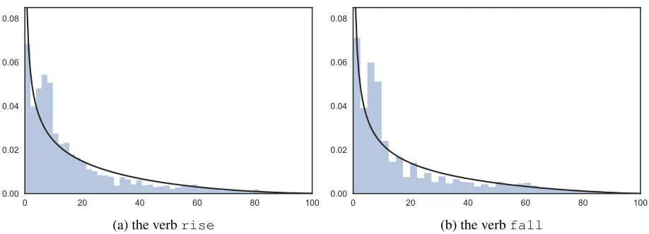
Fig. 3 shows the likelihood functionP(x|w)fitted by KDE with Gaussian kernels and automatic band-width determination using the rule of Scott (2015),
for the most popular upward and downward verbs in the WSJ corpus:riseandfall.
[image:7.612.74.537.388.553.2]
(a) the verbrise
[image:8.612.76.530.57.220.2]
(b) the verbfall
Figure 3: The likelihood functionP(x|w)fitted by kernel density estimation (KDE).
(a) the verbrise
(b) the verbfall
Figure 4: The likelihood functionP(x|w)fitted by the Beta distribution.
distribution which is a continuous distribution sup-ported on the bounded interval[0,1]:
P(x|w) =Beta(α, β) = Γ(α+β)
Γ(α)Γ(β)x
α−1(1−x)β−1. (8)
Although there exist a number of continuous dis-tributions supported on the bounded interval such as the truncated normal distribution, the Beta dis-tribution is picked here as it has the ability to take a great variety of different shapes using only two parametersαandβ. These two parameters can be es-timated using the method of moments, or maximum likelihood. For example, using the former, we have
b
α= ¯xx¯(1¯v−x¯) −1andβb= (1−x)¯ x¯(1¯v−x¯) −1
if¯v <x(1¯ −x), where¯ x¯andv¯are the sample mean
and sample variance respectively. Fig. 4 shows the
likelihood function P(x|w) fitted by the Beta dis-tribution using SciPy4for the most popular upward and downward verbs in the WSJ corpus:riseand fall.
5 Experiments 5.1 Baselines
Thomson Reuters: The only published approach that we are aware of to this specific task of verb selec-tion in the context of data-to-text NLG is the method adopted by Thomson Reuters EikonTM (Smiley et al., 2016). This baseline method’s effectiveness has been verified through crowdsourcing, as we have mentioned before (see Section 2). Furthermore, it is fairly new (published in 2016), therefore should
[image:8.612.74.533.255.421.2]represent the state of the art in this field. Note that their model was not taken off-the-shelf but re-trained on our datasets to ensure a fair comparison with our approach.
Neural Network: Another baseline method that we have tried is a feed-forward artificial neural net-work with hidden layers, aka, amulti-layer percep-tron(Russell and Norvig, 2009; Goodfellow et al., 2016). It is because neural networks are well-known universal function approximators, and they represent quite a different family of supervised learning algo-rithms. Unlike our proposed probabilistic approach which is essentially agenerative model, the neural network used in our experiments is a discrimina-tive model which takes the percentage change in-put (represented as a single floating-point number) and then predicts the verb choice directly. Since we would like to have probability estimates for each verb, the softmax function was used for the output layer of neurons, and the network was trained via back-propagation to minimize the cross-entropy loss function. Anl2 regularization term was also added
to the loss function that would shrink model param-eters to prevent overfitting. The activation function was set to the rectified linear unit (ReLU) (Hahn-loser et al., 2000). The Adam optimization algo-rithm (Kingma and Ba, 2014) was employed as the solver, with the samples shuffled after each iteration. The initial learning rate was set to 0.001, and the maximum number of iterations (epochs) was set to 1500. For our datasets, a single hidden layer of 100 neurons would be sufficient and adding more neu-rons or layers could not help. This was found using the development set through a line search from 20 to 500 hidden neurons with step size 20. Note that when applying the trained neural network to select verbs, we should use not argmax but sampling from the predicted probability distribution (given by the softmax function), in the same way as we do in our proposed probabilistic model (see Section 4).
5.2 Code
The Python code for our experiments, along with the datasets of verb-percentage pairs extracted from those three corpora (see Section 3), have been made available to the research community5.
5https://goo.gl/gkj8Fa
5.3 Automatic Evaluation
The end users’ perception of a verb selection algo-rithm’s quality depends on not only how accurately the chosen verbs reflect the corresponding percent-age changes but also how diverse the chosen verbs are, which are two largely orthogonal dimensions for evaluation.
Accuracy: The easiest way to assess the accuracy of an NLG method or system is to compare the texts generated by computers and the texts written by hu-mans for the same input data (Mellish and Dale, 1998; Reiter and Belz, 2009), using an automatic metric such as BLEU (Papineni et al., 2002). For our task of verb selection, we decide to use the metric MRR that stands for mean reciprocal rank (Voorhees, 1999; Radev et al., 2002) and can be calculated as follows:
MRR= 1 |Q|
X
(x0 i,w0i)∈Q
1
rank(w0
i)
, (9)
whereQ ={(x01, w01), . . . ,(x0M, wM0 )}is the set of test examples, andrank(w0i)refers to the rank po-sition ofw0i — the verb really used by the human author to describe the percentage change x0i — in the list of predicted verbs ranked in the descending order of their probabilities of correctness given by the model. The MRR metric is most widely used for the evaluation of automatic question answering which is similar to automatic verb selection in the following sense: they both aim to output just one suitable response (answer or verb) to any given input (question or percentage change).
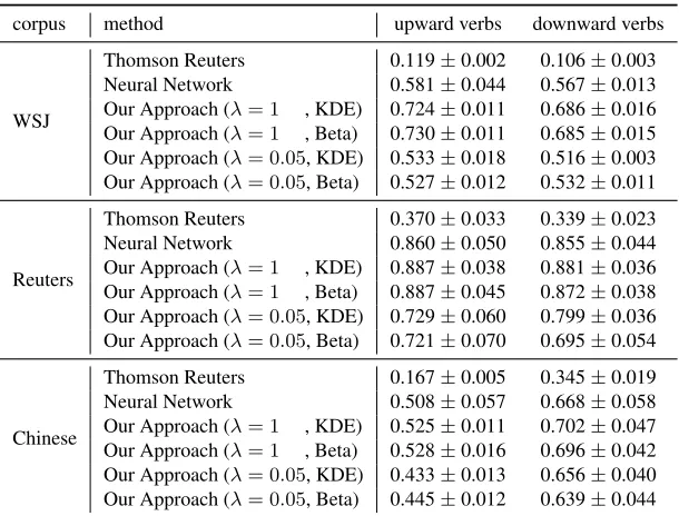
Through 5-fold cross-validation (Hastie et al., 2009), we have got the MRR scores of our proposed model (see Section 4) and the two baseline mod-els (see Section 5.1) which are shown in Table 2. The models were trained/testedseparatelyon each dataset (see Section 3). In each round of 5-fold cross-validation, 20% of the data would become the test set; in the remaining 80% of the data, randomly selected 60% would be the training set and the other 20% would be the development set if parameter tuning is needed (otherwise the whole 80% would be used for training).
corpus method upward verbs downward verbs
WSJ
Thomson Reuters 0.119±0.002 0.106±0.003
Neural Network 0.581±0.044 0.567±0.013
Our Approach (λ= 1 , KDE) 0.724±0.011 0.686±0.016
Our Approach (λ= 1 , Beta) 0.730±0.011 0.685±0.015
Our Approach (λ= 0.05, KDE) 0.533±0.018 0.516±0.003
Our Approach (λ= 0.05, Beta) 0.527±0.012 0.532±0.011
Reuters
Thomson Reuters 0.370±0.033 0.339±0.023
Neural Network 0.860±0.050 0.855±0.044
Our Approach (λ= 1 , KDE) 0.887±0.038 0.881±0.036
Our Approach (λ= 1 , Beta) 0.887±0.045 0.872±0.038
Our Approach (λ= 0.05, KDE) 0.729±0.060 0.799±0.036
Our Approach (λ= 0.05, Beta) 0.721±0.070 0.695±0.054
Chinese
Thomson Reuters 0.167±0.005 0.345±0.019
Neural Network 0.508±0.057 0.668±0.058
Our Approach (λ= 1 , KDE) 0.525±0.011 0.702±0.047
Our Approach (λ= 1 , Beta) 0.528±0.016 0.696±0.042
Our Approach (λ= 0.05, KDE) 0.433±0.013 0.656±0.040
[image:10.612.154.459.53.285.2]Our Approach (λ= 0.05, Beta) 0.445±0.012 0.639±0.044
Table 2: The accuracy of verb selection measured by MRR (mean±std) via 5-fold cross-validation.
only and ignore the diversity, the optimal value of λshould just be 1 (i.e., no smoothing). In order to strike a healthy balance between accuracy and diver-sity, we carried out a line search for the value ofλ from 0 to 1 with step size 0.05 using the development set. It turned out that the smoothing effect upon diver-sity would only become noticeable whenλ≤0.1, so we further conducted a line search from 0 to 0.1 with step size 0.01, and found that usingλ= 0.05 consis-tently yield a good performance on different corpora. Actually, this phenomenon should not be very sur-prising, given the Zipfian distribution of verbs which is highly skewed (see Fig. 1). Our observation in the experiments still indicate that smoothing with a none-zeroλworked better than settingλ= 0. That is to say, it would not be wise to go to extremes to ignore the prior entirely which would unnecessarily harm the accuracy. An alternative smoothing solution for mitigating the severe skewness of the empirical prior that we also considered is to make the smoothed prior probability proportional to the logarithm of the raw prior probability, but we did not take that route as (i) we could not find a good principled interpreta-tion for such a trick and; (ii) using a smallλvalue like 0.05 seemed to work sufficiently well. It will be shown later that sampling verbs from the posterior probability distribution rather than just using the one
with the maximum probability would help to alleviate the problem of prior skewness and thus prevent verb selection from being dominated by the most popular verbs.
It can be observed from the experimental results that smoothing (see Section 4.1) does reduce the accuracy of verb selection. The MRR scores with λ = 0.05 are lower than those with λ = 1. Nev-ertheless, as we shall soon see, strong smoothing is crucially important for achieving a good level of diversity. Furthermore, there seemed to be little per-formance difference between the usage of the KDE technique or the Beta distribution to fit the likelihood function in our approach. This suggests that the latter is preferable because it is as effective as the former but much more efficient. Therefore, in the remaining part of this paper, we shall focus on this specific ver-sion of our model (withλ= 0.05, Beta) even though it may not be the most accurate.
margin in terms of MRR. According to the Wilcoxon signed-rank test (Wilcoxon, 1945; Kerby, 2014), the performance improvements brought by our approach over the Thomson Reuters baseline are statistically significant with the (two-sided)p-value 0.0001 on the two English corpora and= 0.0027 on the Chinese corpus.
With respect to the Neural Network baseline, on all the three corpora, its accuracy is slightly better than that of our smoothed model (λ= 0.05) though it still could not beat our original unsmoothed model (λ = 1). The major problem with the Neural Net-work baseline is that, similar to the probabilistic model without smoothing, its verb choices would concentrate on the most frequent ones and thus have very poor diversity. A prominent advantage of our proposed probabilistic model, in comparison with discriminative learning algorithms such as the Neural Network baseline, is that we are able to explicitly control the trade-off between accuracy and diversity by adjusting the strength of smoothing.
It is worth emphasizing that the accuracy of a verb selection method only reflects its ability to imitate how writers(journalists) use verbs, but this is not necessarily the same as how readers interpret the verbs. Usually the ultimate goal of an NLG sys-tem is to successfully communicate information to readers. Previous research in NLG and psychology suggests that there is wide variation in how different people interpret verbs and words in general, which is probably much larger in the general population than amongst journalists. Specifically, the MRR metric would probably underestimate the effectiveness of a verb selection method, since a verb different from the one really used by the writer is not necessarily a less appropriate choice for the corresponding percentage change from the reader’s perspective.
Diversity: Other than the accuracy of reproducing the verb choices made by human authors, verb selec-tion methods could also be automatically evaluated in terms of diversity.
Following Kingrani et al. (2015), we borrow the diversity measures from ecology (Magurran, 1988) to quantitatively analyze the diversity of verb choices: each specific verb is considered as a particular species. When measuring the biological diversity of a habitant, it is important to consider not only the
number of distinct species present but also the rela-tive abundance of each species. In the literature of ecology, the former is calledrichnessand the latter is calledevenness. Here we utilize the well-known Inverse Simpson Index aka Simpson’s Reciprocal In-dex (Simpson, 1949) which takes both richness and evenness into account: D = PRi=1p2i−1, where Ris the total number of distinct species (i.e., rich-ness), andpiis the the proportion of the individuals belonging to the i-th species relative to the entire population. The evenness is given by the value of diversity normalized to the range between 0 and 1, so it can be calculated asD/R.
Table 3 shows the diversity scores of verb choices made by our approach and the Thomson Reuters base-line for 450 randomly sampled percentage changes (see Section 5.4). Overall, in terms of diversity, our approach would lose to Thomson Reuters. The Neu-ral Network baseline is omitted here because its di-versity scores were very low.
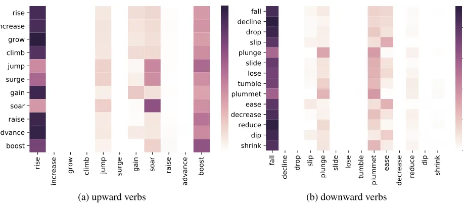
Discussion: Figs. 5 and 6 show the confusion ma-trices of our approach (λ= 0.05, Beta) on the WSJ corpus as (row-normalized) heatmaps: in the former we choose the verb with the highest posterior proba-bility (argmax) while in the latter we sample the verb from the posterior probability distribution (see Sec-tion 4). The argmax way would be dominated by a few verbs (e.g., “rise”, “soar”, “fall”, and “plummet”). In contrast, random sampling would lead to a much wider variety of verbs. The experimental results of all verb selection methods reported in this paper are generated by the sampling strategy, if not indicated otherwise. It can be seen from Fig. 6 that the verbs “soar” and “plunge” are the easiest to be predicted.
Generally speaking, the prediction of verbs is rela-tively more accurate for bigger percentage changes, whether upwards or downwards. This is probably be-cause there are fewer verbs available to describe such radical percentage changes (see Fig. 2) and thus the model faces less uncertainty. Most misclassification (confusion) happens when a verb is incorrectly pre-dicted to be the most frequent one (“rise” or “fall”).
5.4 Human Evaluation
car-rise
increase grow climb jump surge
gain soar raise advance boost
rise increase grow climb jump surge gain soar raise advance
boost 0.0
0.1 0.2 0.3 0.4 0.5
(a) upward verbs
fall
decline drop slip plunge slide lose tumble plummet ease decrease reduce
dip
shrink
fall decline drop slip plunge slide lose tumble plummet ease decrease reduce dip
shrink 0.00
0.15 0.30 0.45 0.60
[image:12.612.79.537.50.253.2](b) downward verbs
Figure 5: The confusion matrix heatmap of our approach on the WSJ corpus: choosing the verb with the highest posterior probability.
rise
increase grow climb jump surge
gain soar raise advance boost
rise increase grow climb jump surge gain soar raise advance boost
0.08 0.10 0.12 0.14 0.16
(a) upward verbs
fall
decline drop slip plunge slide lose tumble plummet ease decrease reduce dip shrink
fall decline drop slip plunge slide lose tumble plummet ease decrease reduce dip
shrink 0.045
0.060 0.075 0.090 0.105 0.120
[image:12.612.75.536.300.499.2](b) downward verbs
Figure 6: The confusion matrix heatmap of our approach on the WSJ corpus: sampling the verb from the posterior probability distribution.
corpus method richness upward verbsevenness diversity richnessdownward verbsevenness diversity
WSJ Our ApproachThomson Reuters 115 0.63240.8771 3.1629.648 145 0.46980.6821 2.3499.550
Reuters Our Approach 3 0.7520 2.256 3 0.5933 1.780
Thomson Reuters 4 0.6453 2.581 4 0.5720 2.288
Chinese Our ApproachThomson Reuters 146 0.79650.5831 4.7798.164 44 0.52650.7150 2.1062.860
[image:12.612.117.496.547.647.2]corpus verbs Our Approach vs Thomson Reuters Our Approach vs Neural Network
> < ≈ p-value > < ≈ p-value
WSJ
upward 43 32 0 0.2480 53 22 0 0.0004
downward 44 28 3 0.0764 42 32 1 0.2954
both 87 60 3 0.0316 95 54 1 0.0010
Reuters
upward 37 28 10 0.3211 43 24 8 0.0271
downward 39 31 5 0.4030 50 23 2 0.0021
both 76 59 15 0.1683 93 47 10 0.0001
Chinese
upward 42 30 3 0.1945 65 9 1 0.0001
downward 29 37 9 0.3891 37 34 4 0.8126
both 71 67 12 0.7985 102 43 5 0.0001
[image:13.612.123.491.55.204.2]All both 234 186 30 0.0217 290 144 16 0.0001
Table 4: The results of human evaluation, where thep-values are given by the sign test (two-sided).
ried out for either accuracy or diversity alone, there is no obvious way to assess the overall effectiveness of a verb selection method using machines only. The ultimate judgment on the quality of verb selection would have to come from human assessors (Mellish and Dale, 1998; Reiter and Belz, 2009; Smiley et al., 2016).
To manually compare our approach (the version withλ= 0.05, Beta) with a baseline method (Thom-son Reuters or Neural Network), we conduct a ques-tionnaire survey with 450 multiple-choice questions. In each question, a respondent would see a pair of generated sentences describing the same percentage change with the verbs selected by two different meth-ods respectively and need to judge which one sounds better than the other (or it is hard to tell). For exam-ple, a respondent could be shown the following pair of generated sentences:
(1) Net profit declines 3% (2) Net profit plummets 3%
and then they were supposed to choose one of the three following options as their answer:
[a] Sentence (1) sounds better. [b] Sentence (2) sounds better. [c] They are equally good.
The respondents would beblindedto whether the first verb or the second verb was provided by our proposed method, as their appearing order would have been randomized in advance. The questionnaire survey system withheld the information about the source of each verb until the answers from all respondents had been collected, and then it would count how many times the verb selected by our proposed method was
deemed better than (>), worse than (<), or as good as (≈) the verb selected by the baseline method.
For each corpus, we produced 150 different ques-tions, of which half were about upward verbs and half were about downward verbs. As we have explained above, each question compares a pair of generated sentences describing the same percentage change with different verbs. The sentence generation process is the same as that used by Smiley et al. (2016). The
subjectswere randomly picked from the most popular ones in the corpus (e.g., “gross domestic product”), and the percentage changes (as theobjects) were ran-domly sampled from the corpus as well. Each of the two verb selection methods, in comparison, would provide one verb (as thepredicate) for describing that specific percentage change. Note that in this sentence generation process, a pair of sentences would be re-tained only if the verbs selected by the two methods were different, as it would be meaningless to compare two identical sentences.
A total of 15 college-educated people participated in the questionnaire survey. They are all bilingual, i.e., native or fluent speakers of both English and Chinese. Each person was given 30 questions: 10 questions (including 5 upward and 5 downward ones) from each corpus. We (the authors of this paper) were excluded from participating in the questionnaire survey to avoid any conscious or unconscious bias.
our approach 290/450=64% of times, as opposed to 144/450=32% for the Neural Network baseline. According to thesign test (Wackerly et al., 2007), our approach works significantly better than the two baseline methods, Thomson Reuters and Neural Net-work: overall the (two-sided)p-values are less than 0.05.
Discussion: Our approach exhibits more superior-ity over the Thomson Reuters baseline on the English datasets than on the Chinese dataset. Since the Chi-nese dataset is bigger than the Reuters dataset, though smaller than the WSJ dataset, the performance differ-ence is not caused by corpus size but due to language characteristics. Remember that for Chinese we are actually predicting adverb+verb combinations (see Section 3.3). Retrospective manual inspection of the experimental results suggests that users seem to have relatively higher expectations of diversity for Chinese adverbs than for English verbs.
6 Extensions
Robustness: It is still possible, though very un-likely, for the proposed probabilistic model to gen-erate atypical uses of a verb. A simple measure to avoid such situations is to reject the sampled verbw∗ if the posterior probabilityP(w∗|x)< τ whereτ is a predefined threshold, e.g., 5%, and then resample w∗untilP(w∗|x)≥τ.
Unlimited Range: If the magnitude of a percent-age change is allowed to go beyond100%, we would no longer be able to use the Beta distribution to fit the likelihood functionP(x|w)as it is supported on a bounded interval. However, it should be straight-forward to use a flexible probability distribution sup-ported on the semi-infinite interval[0,+∞], such as the Gamma distribution.
Subject: The context, in particular the subject of the percentage change, has not been taken into ac-count by the presented models. As illustrated by the two example sentences below, the same verb (“surge”) could be used for quite different percentage changes (“181%” vs “8%”) depending on the subject (“wheat price” vs “inflation”).
• “According to World Bank figures, wheat prices have surged up by 181 percent in the past three years to February 2008.”
• “While inflation has surged to almost 8% in 2008, it is projected by the Commission to fall in 2009.” Furthermore, the significance of a percentage change often depends on the domain, and consequently, so does the most appropriate verb to describe a per-centage change. For example, a 10% increase in stock price is interesting, while a 10% increase in body temperature is life-threatening. It is, of course, possible to incorporate the subject information into our probabilistic model by extending Eq. (2) to
P(w|x, s) = P(w, s)P(x|w, s)/P(x, s)wheresis
the subject word in the triple. On one hand, this should make the model more effective, for the rea-sons explained above. On the other hand, this would require a lot more data for reliable estimation of the model parameters, which is one of the reasons why we leave it for future work.
Language Modeling: Thanks to its probabilistic nature, our proposed model for verb selection could be seamlessly plugged into ann-gram statistical lan-guage model (Jurafsky and Martin, 2009), e.g., for the MSR Sentence Completion Challenge6. This might be able to reduce the language model’s perplex-ity, as the probability ofhsubject,verb,percentagei triples could be calculated more precisely.
Hierarchical Modeling: The choice of verb to de-scribe a particular percentage change could be af-fected by the style of the author, the topic of the document, and other contextual factors. To take those dimensions into account and build a finer prob-abilistic model for verb selection, we could embrace
Bayesian hierarchical modeling(Gelman et al., 2013; Kruschke, 2014) which, for example, could let each author’s model borrow the “statistical power” from other authors’.
Psychology: There exist a lot of studies in psy-chology on how people interpret probabilities and risks (Reagan et al., 1989; Berry et al., 2004). They could provide useful insights for further enhancing our verb selection method.
7 Conclusions
The major research contribution of this paper is a probabilistic model that can select appropriate verbs
to express percentage changes with different direc-tions and magnitudes. This model is not relying on hard-wired heuristics, but learned from training ex-amples (in the form of verb-percentage pairs) that are extracted from large-scale real-world news corpora. The choices of verbs made by the proposed model are found to match our intuitions about how differ-ent verbs are collocated with percdiffer-entage changes of different sizes. The real challenge here is to strike the right balance between accuracy and diversity, which can be realized via smoothing. Our experi-ments have confirmed that the proposed model can capture human authors’ pattern of usage around verbs better than the existing method currently employed by Thomson Reuters EikonTM. We hope that this probabilistic model for verb selection could help data-to-text NLG systems achieve greater variation and naturalness.
Acknowledgments
The research is partly funded by the National Key R&D Program of China (ID: 2017YFC0803700) and the NSFC grant (No. 61532021). The Titan X Pascal GPU used for our experiments was kindly donated by the NVIDIA Corporation. Prof Xuanjing Huang (Fudan) has helped with the datasets.
We thank the anonymous reviewers and the ac-tion editor for their constructive and helpful com-ments. We also gratefully acknowledge the support of Geek.AI for this work.
References
Lada A Adamic. 2000. Zipf, power-laws, and Pareto — A ranking tutorial. Technical report, HP Labs. Gabor Angeli, Percy Liang, and Dan Klein. 2010. A
simple domain-independent probabilistic approach to generation. InProceedings of the 2010 Conference on Empirical Methods in Natural Language Processing (EMNLP), pages 502–512.
Anja Belz and Eric Kow. 2009. System building cost vs. output quality in data-to-text generation. In Pro-ceedings of the 12th European Workshop on Natural Language Generation (ENLG), pages 16–24.
Anja Belz. 2008. Automatic generation of weather fore-cast texts using comprehensive probabilistic generation-space models. Natural Language Engineering (NLE), 14(04):431–455.
Dianne Berry, Theo Raynor, Peter Knapp, and Elisabetta Bersellini. 2004. Over the counter medicines and the need for immediate action: A further evaluation of Eu-ropean Commission recommended wordings for com-municating risk. Patient Education and Counseling, 53(2):129–134.
Steven Bird, Ewan Klein, and Edward Loper. 2009. Natu-ral Language Processing with Python: Analyzing Text with the Natural Language Toolkit. O’Reilly Media. Sarah Boyd. 1998. TREND: A system for generating
intelligent descriptions of time series data. In Pro-ceedings of the 2nd IEEE International Conference on Intelligent Processing Systems (ICIPS).
Eugene Charniak, Don Blaheta, Niyu Ge, Keith Hall, John Hale, and Mark Johnson. 2000. BLLIP 1987-89 WSJ Corpus Release 1 LDC2000T43. Web Download. Philadelphia: Linguistic Data Consortium.
Andrew Gelman, John Carlin, Hal Stern, David Dunson, Aki Vehtari, and Donald Rubin. 2013.Bayesian Data Analysis. CRC, 3rd edition.
Eli Goldberg, Norbert Driedger, and Richard I. Kittredge. 1994. Using natural-language processing to produce weather forecasts.IEEE Expert, 9(2):45–53.
Ian Goodfellow, Yoshua Bengio, and Aaron Courville. 2016.Deep Learning. MIT Press.
Richard H.R. Hahnloser, Rahul Sarpeshkar, Misha A. Ma-howald, Rodney J. Douglas, and H. Sebastian Seung. 2000. Digital selection and analogue amplification coexist in a cortex-inspired silicon circuit. Nature, 405(6789):947–951.
Trevor Hastie, Robert Tibshirani, and Jerome Friedman. 2009. The Elements of Statistical Learning: Data Min-ing, Inference, and Prediction. Springer, 2nd edition. Frederick Jelinek and Robert Mercer, 1980.Interpolated
Estimation of Markov Source Parameters from Sparse Data, pages 381–402. North-Holland Publishing. Daniel Jurafsky and James H. Martin. 2009. Speech
and Language Processing: An Introduction to Natural Language Processing, Computational Linguistics and Speech Recognition. Prentice Hall, 2nd edition. Dave S Kerby. 2014. The simple difference formula: An
approach to teaching nonparametric correlation. Com-prehensive Psychology, 3(1).
Diederik P. Kingma and Jimmy Ba. 2014. Adam: A method for stochastic optimization. arXiv preprint arXiv:1412.6980.
Suneel Kumar Kingrani, Mark Levene, and Dell Zhang. 2015. Diversity analysis of web search results. In Pro-ceedings of the Annual International ACM Web Science conference (WebSci).
Manfred Krifka. 2007. Approximate interpretations of number words: A case for strategic communication. InCognitive Foundations of Interpretation, pages 111– 126.
John K Kruschke. 2014. Doing Bayesian Data Analysis: A Tutorial with R, JAGS, and Stan. Academic Press, 2nd edition.
Anne E. Magurran. 1988. Ecological Diversity and Its Measurement. Princeton University Press.
Christopher D. Manning, Prabhakar Raghavan, and Hin-rich Sch¨utze. 2008. Introduction to Information Re-trieval. Cambridge University Press.
Christopher D. Manning, Mihai Surdeanu, John Bauer, Jenny Rose Finkel, Steven Bethard, and David Mc-Closky. 2014. The Stanford CoreNLP natural language processing toolkit. InProceedings of the 52nd Annual Meeting of the Association for Computational Linguis-tics (ACL), System Demonstrations, pages 55–60. Hongyuan Mei, Mohit Bansal, and Matthew R. Walter.
2016. What to talk about and how? Selective gen-eration using LSTMs with coarse-to-fine alignment. InProceedings of the 2016 Conference of the North American Chapter of the Association for Computational Linguistics: Human Language Technologies (NAACL-HLT), pages 720–730.
Chris Mellish and Robert Dale. 1998. Evaluation in the context of natural language generation. Computer Speech & Language, 12(4):349–373.
Priscilla Moraes, Kathleen McCoy, and Sandra Carberry. 2014. Adapting graph summaries to the users’ reading levels. InProceedings of the 8th International Natural Language Generation Conference (INLG), pages 64– 73.
Mark E. J. Newman. 2005. Power laws, Pareto distribu-tions and Zipf’s law.Contemporary Physics, 46(5):323– 351.
Kishore Papineni, Salim Roukos, Todd Ward, and Wei-Jing Zhu. 2002. BLEU: A method for automatic evalu-ation of machine translevalu-ation. InProceedings of the 40th Annual Meeting of the Association for Computational Linguistics (ACL), pages 311–318.
Vassilis Plachouras, Charese Smiley, Hiroko Bretz, Ola Taylor, Jochen L. Leidner, Dezhao Song, and Frank Schilder. 2016. Interacting with financial data us-ing natural language. InProceedings of the 39th In-ternational ACM SIGIR Conference on Research and Development in Information Retrieval (SIGIR), pages 1121–1124.
David MW Powers. 1998. Applications and explanations of Zipf’s law. InProceedings of the Joint Conferences on New Methods in Language Processing and Computa-tional Natural Language Learning (NeMLaP/CoNLL), pages 151–160.
Dragomir R. Radev, Hong Qi, Harris Wu, and Weiguo Fan. 2002. Evaluating web-based question answer-ing systems. InProceedings of the 3rd International Conference on Language Resources and Evaluation (LREC).
Alejandro Ramos-Soto, Alberto Bugar´ın, Sen´en Barro, and Juan Taboada. 2013. Automatic generation of textual short-term weather forecasts on real prediction data. InProceedings of the 10th International Confer-ence on Flexible Query Answering Systems (FQAS), pages 269–280.
Josef Raviv. 1967. Decision making in Markov chains applied to the problem of pattern recognition. IEEE Transactions on Information Theory, 13(4):536–551. Robert T. Reagan, Frederick Mosteller, and Cleo Youtz.
1989. Quantitative meanings of verbal probability ex-pressions. Journal of Applied Psychology, 74(3):433. Ehud Reiter and Anja Belz. 2009. An investigation into
the validity of some metrics for automatically evalu-ating natural language generation systems. Computa-tional Linguistics, 35(4):529–558.
Ehud Reiter, Somayajulu Sripada, Jim Hunter, Jin Yu, and Ian Davy. 2005. Choosing words in computer-generated weather forecasts. Artificial Intelligence, 167(1-2):137–169.
Ehud Reiter. 2007. An architecture for data-to-text sys-tems. InProceedings of the 11th European Workshop on Natural Language Generation (ENLG), pages 97– 104.
Stuart Russell and Peter Norvig. 2009. Artificial Intelli-gence: A Modern Approach. Prentice Hall, 3rd edition. David W Scott. 2015. Multivariate Density Estimation: Theory, Practice, and Visualization. John Wiley & Sons.
Claude E. Shannon. 1948. A mathematical theory of com-munication. Bell System Technical Journal, 27:623– 656.
Heung-Yeung Shum, Xiaodong He, and Di Li. 2018. From Eliza to XiaoIce: Challenges and opportunities with social chatbots.arXiv preprint arXiv:1801.01957. Edward H Simpson. 1949. Measurement of diversity.
Nature.
Charese Smiley, Vassilis Plachouras, Frank Schilder, Hi-roko Bretz, Jochen L. Leidner, and Dezhao Song. 2016. When to plummet and when to soar: Corpus based verb selection for natural language generation. In Pro-ceedings of the 9th International Natural Language Generation Conference (INLG), pages 36–39.
Ellen M. Voorhees. 1999. The TREC-8 question an-swering track report. InProceedings of the 8th Text REtrieval Conference (TREC), pages 77–82.
Dennis Wackerly, William Mendenhall, and Richard Scheaffer. 2007.Mathematical Statistics with Applica-tions. Nelson Education.
Frank Wilcoxon. 1945. Individual comparisons by rank-ing methods. Biometrics Bulletin, 1(6):80–83. Alex Wright. 2015. Algorithmic authors.
Communica-tions of the ACM (CACM), 58(11):12–14.