Encoding Prior Knowledge with Eigenword Embeddings
Dominique Osborne
Department of Mathematics and Statistics University of Strathclyde
Glasgow, G1 1XH, UK
Shashi Narayan and Shay B. Cohen School of Informatics
University of Edinburgh Edinburgh, EH8 9LE, UK {snaraya2,scohen}@inf.ed.ac.uk
Abstract
Canonical correlation analysis (CCA) is a method for reducing the dimension of data represented using two views. It has been previously used to derive word embeddings, where one view indicates a word, and the other view indicates its context. We describe a way to incorporate prior knowledge into CCA, give a theoretical justification for it, and test it by deriving word embeddings and evaluating them on a myriad of datasets.
1 Introduction
In recent years there has been an immense in-terest in representing words as low-dimensional continuous real-vectors, namely word embeddings. Word embeddings aim to capture lexico-semantic information such that regularities in the vocabulary are topologically represented in a Euclidean space. Such word embeddings have achieved state-of-the-art performance on many natural language process-ing (NLP) tasks, e.g., syntactic parsprocess-ing (Socher et al., 2013), word or phrase similarity (Mikolov et al., 2013b), dependency parsing (Bansal et al., 2014), unsupervised learning (Parikh et al., 2014) and oth-ers. Since the discovery that word embeddings are useful as features for various NLP tasks, research on word embeddings has taken on a life of its own, with a vibrant community searching for better word rep-resentations in a variety of problems and datasets.
These word embeddings are often induced from large raw text capturing distributional co-occurrence information via neural networks (Bengio et al., 2003; Mikolov et al., 2013b; Mikolov et al., 2013c) or spectral methods (Deerwester et al., 1990; Dhillon et al., 2015). While these general pur-pose word embeddings have achieved significant
im-provement in various tasks in NLP, it has been dis-covered that further tuning of these continuous word representations for specific tasks improves their per-formance by a larger margin. For example, in de-pendency parsing, word embeddings could be tai-lored to capture similarity in terms of context within syntactic parses (Bansal et al., 2014) or they could be refined using semantic lexicons such as WordNet (Miller, 1995), FrameNet (Baker et al., 1998) and the Paraphrase Database (Ganitkevitch et al., 2013) to improve various similarity tasks (Yu and Dredze, 2014; Faruqui et al., 2015; Rothe and Sch¨utze, 2015). This paper proposes a method to encode prior semantic knowledge in spectral word embeddings (Dhillon et al., 2015).
Spectral learning algorithms are of great inter-est for their speed, scalability, theoretical guaran-tees and performance in various NLP applications. These algorithms are no strangers to word embed-dings either. In latent semantic analysis (LSA, (Deerwester et al., 1990; Landauer et al., 1998)), word embeddings are learned by performing SVD on the word by document matrix. Recently, Dhillon et al. (2015) have proposed to use canonical cor-relation analysis (CCA) as a method to learn low-dimensional real vectors, called Eigenwords. Un-like LSA based methods, CCA based methods are scale invariant and can capture multiview informa-tion such as the left and right contexts of the words. As a result, the eigenword embeddings of Dhillon et al. (2015) that were learned using the simple lin-ear methods give accuracies comparable to or better than state of the art when compared with highly non-linear deep learning based approaches (Collobert and Weston, 2008; Mnih and Hinton, 2007; Mikolov et al., 2013b; Mikolov et al., 2013c).
The main contribution of this paper is a technique
417
to incorporate prior knowledge into the derivation of canonical correlation analysis. In contrast to previ-ous work where prior knowledge is introduced in the off-the-shelf embeddings as a post-processing step (Faruqui et al., 2015; Rothe and Sch¨utze, 2015), our approach introduces prior knowledge in the CCA derivation itself. In this way it preserves the the-oretical properties of spectral learning algorithms for learning word embeddings. The prior knowl-edge is based on lexical resources such as WordNet, FrameNet and the Paraphrase Database.
Our derivation of CCA to incorporate prior knowledge is not limited to eigenwords and can be used with CCA for other problems. It follows a sim-ilar idea to the one proposed by Koren and Carmel (2003) for improving the visualization of principal vectors with principal component analysis (PCA). Our derivation represents the solution to CCA as that of an optimization problem which maximizes the distance between the two view projections of training examples, while weighting these distances using the external source of prior knowledge. As such, our approach applies to other uses of CCA in the NLP literature, such as the one of Jagarlamudi and Daum´e (2012), who used CCA for translitera-tion, or the one of Silberer et al. (2013), who used CCA for semantically representing visual attributes.
2 Background and Notation
For an integern, we denote by[n]the set of integers {1, . . . , n}. We assume the existence of a vocabu-lary of words, usually taken from a corpus. This set of words is denoted byH ={h1, . . . , h|H|}. For a square matrixA, we denote bydiag(A) a diagonal
matrixBwhich has the same dimensions asAsuch thatBii =Aiifor alli. For vectorv ∈Rd, we
de-note its`2norm by||v||, i.e.||v||=qPdi=1vi2. We
also denote byvjor[v]j thejth coordinate ofv. For
a pair of vectorsuandv, we denote their dot product byhu, vi.
We define a word embedding as a functionffrom H toRm for some (relatively small)m. For exam-ple, in our experiments we varym between50 and 300. The word embedding function maps the word to some real-vector representation, with the inten-tion to capture regularities in the vocabulary that are topologically represented in the corresponding
Eu-clidean space. For example, all vocabulary words that correspond to city names could be grouped to-gether in that space.
Research on the derivation of word embeddings that capture various regularities has greatly accel-erated in recent years. Various methods used for this purpose range from low-rank approximations of co-occurrence statistics (Deerwester et al., 1990; Dhillon et al., 2015) to neural networks jointly learn-ing a language model (Bengio et al., 2003; Mikolov et al., 2013a) or models for other NLP tasks (Col-lobert and Weston, 2008).
3 Canonical Correlation Analysis for Deriving Word Embeddings
One recent approach to derive word embeddings, developed by Dhillon et al. (2015), is through the use of canonical correlation analysis, resulting in so-called “eigenwords.” CCA is a technique for multi-view dimensionality reduction. It assumes the ex-istence of two views for a set of data, similarly to co-training (Yarowsky, 1995; Blum and Mitchell, 1998), and then projects the data in the two views in a way that maximizes the correlation between the projected views.
Dhillon et al. (2015) used CCA to derive word embeddings through the following procedure. They first break each document in a corpus of documents intonsequences of words of a fixed length2k+ 1,
wherekis a window size. For example, ifk = 2,
the short document “Harry Potter has been a best-seller” would be broken into “Harry Potter has been a” and “Potter has been a best-seller.” In each such sequence, the middle word is identified as a pivot.
This leads to the construction of the fol-lowing training set from a set of documents:
{(w1(i), . . . , w(ki), w(i), wk(i+1) , . . . , w2(ik)) | i ∈ [n]}.
With abuse of notation, this is a multiset, as cer-tain words are expected to appear in cercer-tain contexts multiple times. Eachw(i) is a pivot word, and the rest of the elements are words in the sequence called “the context words.” With this training set in mind, the two views for CCA are defined as following.
corre-|H|
1 2 i n
W
1 0
2 0 0 0
j
w(i)=h j
1 0 0
|H|
0
1 2 i
n 1 k 2k
C
1 0
2 0 0 0
j
wk(i)=hj
1 0 0
|H|
0
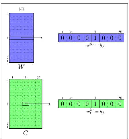
Figure 1: The word and context views represented as ma-trixW andC. Each row inW is a vector of length|H|, corresponding to a one-hot vector for the word in the ex-ample indexed by the row. Each row inC is a vector of length2k|H|, divided into sub-vectors each of length
|H|. Each such sub-vector is a one-hot vector for one of the2kcontext words in the example indexed by the row.
sponds to a word that fired in a specific index in the context. In addition, we also define a second view through a matrixW ∈Rn×|H|such thatWij = 1if
w(i) =hj. We present both views of the training set
in Figure 1.
Note that now the matrix M = W>C is in R|H|×(2k|H|) such that each element M
ij gives the
count of times thathiappeared with the
correspond-ing context word and context index encoded byj. Similarly, we define a matrixD1 = diag(W>W)
andD2 = diag(C>C). Finally, to get the word
em-beddings, we perform singular value decomposition (SVD) on the matrixD−11/2M D2−1/2. Note that in its original form, CCA requires use of W>W and C>Cin their full form, and not just the correspond-ing diagonal matricesD1andD2; however, in
prac-tice, inverting these matrices can be quite intensive computationally and can lead to memory issues. As such, we approximate CCA by using the diagonal matricesD1andD2.
From the SVD step, we get two projectionsU ∈
R|H|×mandV ∈R2k|H|×msuch that
D1−1/2M D2−1/2 ≈UΣV>
where Σ ∈ Rm×m is a diagonal matrix with Σii > 0 being the ith largest singular value of
D1−1/2M D−21/2. In order to get the final word em-beddings, we calculate D−11/2U ∈ R|H|×m. Each
row in this matrix corresponds to anm-dimensional vector for the corresponding word in the vocabulary. This means thatf(hi)forhi ∈ H is theith row of
the matrixD1−1/2U. The projection V can be used to get “context embeddings.” See more about this in Dhillon et al. (2015).
This use of CCA to derive word embeddings follows the usual distributional hypothesis (Harris, 1957) that most word embeddings techniques rely on. In the case of CCA, this hypothesis is trans-lated into action in the following way. CCA finds projections for the contexts and for the pivot words which are most correlated. This means that if a word co-occurs in a specific context many times (either directly, or transitively through similarity to other words), then this context is expected to be projected to a point “close” to the point to which the word is projected. As such, if two words occur in a specific context many times, these two words are expected to be projected to points which are close to each other. For the next section, we denote X = W D−11/2 andY = CD2−1/2. To refer to the dimensions of XandY generically, we denoted= |H|andd0 = 2k|H|. In addition, we refer to the column vectors ofU andV asu1, . . . , umandv1, . . . , vm.
Mathematical Intuition Behind CCA The
pro-cedure that CCA follows finds a projection of the two views in a shared space, such that the correla-tion between the two views is maximized at each co-ordinate, and there is minimal redundancy between the coordinates of each view. This means that CCA solves the following sequence of optimization prob-lems forj∈[m]whereaj ∈R1×dandbj ∈R1×d0:
arg max aj,bj
corr(ajW>, bjC>)
where corr is a function that accepts two vectors and return the Pearson correlation between the pair-wise elements of the two vectors. The approxi-mate solution to this optimization problem (when using diagonal D1 andD2) isaˆ>i = D−
1/2 1 ui and ˆb>
i =D−
1/2
2 vifori∈[m].
CCA also has a probabilistic interpretation as a maximum likelihood solution of a latent variable model for two normal random vectors, each drawn based on a third latent Gaussian vector (Bach and Jordan, 2005).
The way we describe CCA for deriving word embeddings is related to Latent Semantic Indexing (LSI), which performs singular value decomposition on the matrix M directly, without doing any kind of variance normalization. Dhillon et al. (2015) de-scribe some differences between LSI and CCA. The extra normalization step decreases the importance of frequent words when doing SVD.
4 Incorporating Prior Knowledge into Canonical Correlation Analysis
In this section, we detail the technique we use to incorporate prior knowledge into the derivation of canonical correlation analysis. The main motiva-tion behind our approach is to improve the opti-mization of correlation between the two views by weighing them using the external source of prior knowledge. The prior knowledge is based on lex-ical resources such as WordNet, FrameNet and the Paraphrase Database. Our approach follows a sim-ilar idea to the one proposed by Koren and Carmel (2003) for improving the visualization of principal vectors with principal component analysis (PCA). It is also related to Laplacian manifold regularization (Belkin et al., 2006).
An important notion in our derivation is that of a
Laplacian matrix. The Laplacian of an undirected
weighted graph is ann×n matrix where n is the number of nodes in the graph. It equalsD−Awhere Ais the adjacency matrix of the graph (so thatAijis
the weight for the edge(i, j)in the graph, if it exists,
and 0 otherwise) and D is a diagonal matrix such thatDii=PjAij. The Laplacian is always a
sym-metric square matrix such that the sum over rows (or columns) is0. It is also positive semi-definite.
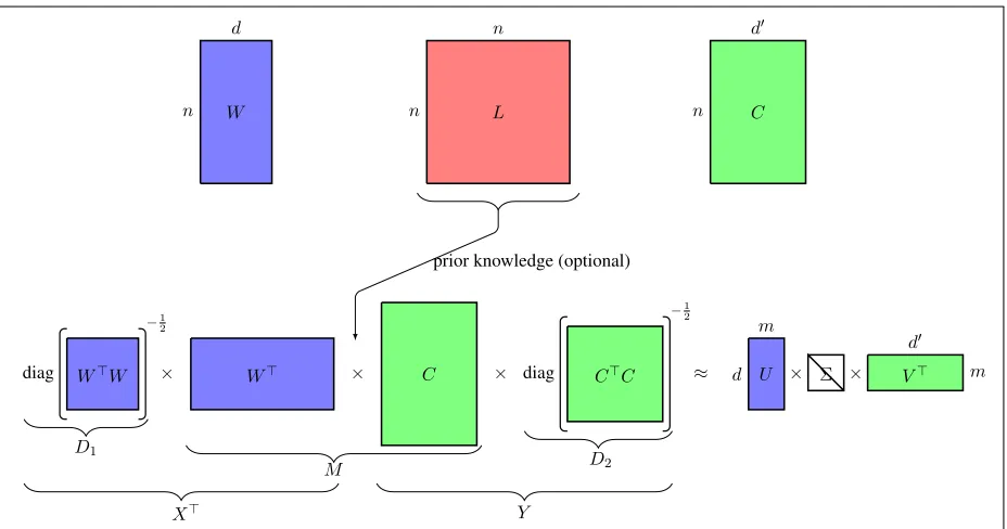
We propose a generalization of CCA, in which we
introduce a Laplacian matrix into the derivation of CCA itself, as shown in Figure 2. We encode prior knowledge about the distances between the projec-tions of two views into the Laplacian. The Laplacian allows us to improve the optimization of the correla-tion between the two views by weighing them using the external source of prior knowledge.
4.1 Generalization of CCA
We present three lemmas (proofs are given in Ap-pendix A), followed by our main proposition. These three lemmas are useful to prove our final proposi-tion.
The main proposition shows that CCA maximizes the distance between the two view projections for any pair of examples iand j, i 6= j, while mini-mizing the two view projection distance for the two views of an examplei. The two views we discuss here in practice are the view of the word through a one-hot representation, and the view which repre-sents the context words for a specific word token. The distance between two view projections is de-fined in Eq. 2.
Lemma 1. LetXandY be two matrices of sizen×d
andn×d0, respectively, for example, as defined in
§3. Assume that Pni=1Xij = 0 for j ∈ [d] and
Pn
i=1Yij = 0 for j ∈ [d0]. Let L be an n×n
Laplacian matrix such that
Lij = (
n−1 ifi=j
−1 ifi6=j. (1)
ThenX>LY equalsX>Y up to a multiplication by
a positive constant.
Lemma 2. LetA ∈ Rd×d0
. Then the rankm
thin-SVD ofAcan be found by solving the following
op-timization problem:
max
u1, . . . , um,
v1, . . . , vm m X
i=1
u>i Avi
such that||ui||=||vi||= 1 i∈[m]
hui, uji=hvi, vji= 0 i6=j
where ui ∈ Rd×1 denote the left singular vectors,
d
n W
n
n L
prior knowledge (optional)
d0
n C
diag W>W −1
2
D1
× W> × C ×
M
diag C>C −1
2
D2
≈
m
d U × Σ ×
d0
m V>
[image:5.612.75.539.52.296.2]X> Y
Figure 2: Introducing prior knowledge in CCA.W ∈ Rn×d andC
∈ Rn×d0
denote the word and context views respectively. L ∈ Rn×n is a Laplacian matrix encoded with the prior knowledge about the distances between the
projections ofW andC.
The last utility lemma we describe shows that in-terjecting the Laplacian between the two views can be expressed as a weighted sum of the distances be-tween the projections of the two views (these dis-tances are given in Eq. 2), where the weights come from the Laplacian.
Lemma 3. Let u1, . . . , um and v1, . . . , vm be two
sets of vectors of lengthdandd0 respectively. Let
L∈Rn×nbe a Laplacian andX ∈Rn×dandY ∈
Rn×d0
. Then:
m X
k=1
(Xuk)>L(Y vk) = X
i,j
−Lij dmij 2
,
where
dmij = v u u
t1
2 m X
k=1
([Xuk]i−[Y vk]j)2 !
. (2)
The following proposition is our main result for this section.
Proposition 4. The matricesU ∈ Rd×m andV ∈
Rd0×m
that CCA computes are the m-dimensional
projections that maximize
X
i,j
dmij2−n
n X
i=1
(dmii)2, (3)
wheredm
ij is defined as in Eq.2foru1, . . . , umbeing
the columns ofU andv1, . . . , vmbeing the columns
ofV.
Proof. According to Lemma 3, the objective in Eq. 3
equalsPm
k=1(Xuk)>L(Y vk)whereLis defined as
in Eq. 1. Therefore, maximizing Eq. 3 corresponds to maximization ofPm
k=1(Xuk)>L(Y vk)under the
constraints that theUandV matrices have orthonor-mal vectors. Using Lemma 2, it can be shown that the solution to this maximization is done by doing singular value decomposition onX>LY. Accord-ing to Lemma 1, this corresponds to findAccord-ingU and V by doing singular value decomposition onX>Y, because a multiplicative constant does not change the value of the right/left singular vectors.
minimizing the distance between the projections of the two views for a specific example (second term in Eq. 3). Therefore, CCA tries to project a context and a word in that context to points that are close to each other in a shared space, while maximizing the distance between a context and a word which do not often co-occur together.
As long asLis a Laplacian, Proposition 4 is still true, only with the maximization of the objective
X
i,j
−Lij dmij 2
, (4)
whereLij ≤ 0fori 6= j andLii ≥ 0. This result
lends itself to a generalization of CCA, in which we use predefined weights for the Laplacian that encode some prior knowledge about the distances that the projections of two views should satisfy.
If the weight −Lij is large for a specific (i, j),
then we will try harder to maximize the distance be-tween one view of exampleiand the other view of examplej(i.e. we will try to project the wordw(i) and the context of examplej into distant points in the space).
This means that in the current formulation,−Lij
plays the role of a dissimiliarity indicator between pairs of words. The more dissimilar words are, the larger the weight, and then the more distant the pro-jections are for the contexts and the words.
4.2 From CCA with Dissimilarities to CCA with Similarities
It is often more convenient to work withsimilarity
measures between pairs of words. To do that, we can retain the same formulation as before with the Laplacian, where −Lij now denotes a measure of
similarity. Now, instead of maximizing the objective in Eq. 4, we are required to minimize it.
It can be shown that such mirror formulation can be done with an algorithm similar to CCA, leading to a proposition in the style of Proposition 4. To solve this minimization formulation, we just need to choose the singular vectors associated with the
smallestmsingular values (instead of the largest).
Once we change the CCA algorithm with the Laplacian to choose these projections, we can de-fineL, for example, based on a similarity graph. The graph is an undirected graph that has|H|nodes, for
Inputs: Set of examples
{(w(1i), . . . , w (i) k , w(i), w
(i)
k+1, . . . , w (i)
2k) | i ∈ [n]}, an
integerm, anα∈ (0,1], an undirected graphGover H, an integerN.
Data structures:
A matrixMof size|H| ×(2k|H|)(cross-covariance matrix), a matrixUcorresponding to the word embed-dings
Algorithm:
(Cross-covariance estimation)∀i, j∈[n]such that|i− j| ≤N
• Ifi = j, increaseMrsby1 forrdenoting the
in-dex of wordw(i)and for allsdenoting the context indices of wordsw(1i), . . . , w
(i) k andw
(i)
k+1, . . . , w (i) 2k. • Ifi 6= j and wordw(i)is connected to wordw(j) inG, increaseMrsbyαforrdenoting the index of
wordw(i)and for allsdenoting the context indices of wordsw(1j), . . . , w
(j) k andw
(j)
k+1, . . . , w (j) 2k.
• CalculateD1andD2as specified in§3. (Singular value decomposition step)
• Perform singular value decomposition on D1−1/2M D−
1/2
2 to get a matrixU ∈R|H|×m. (Word embedding projection)
• For each wordhifori∈[|H|]return the word
em-bedding that corresponds with theith row ofU.
Figure 3: The CCA-like algorithm that returns word em-beddings with prior knowledge encoded based on a simi-larity graph.
each word in the vocabulary, and there is an edge be-tween a pair of words whenever the two words are similar to each other based on some external source of information, such as WordNet (for example, if they are synonyms).
We then define the Laplacian Lsuch that Lij = −1ifiandjare adjacent in the graph (andi 6=j), Lii is the degree of the nodei andLij = 0in all
4.3 Final Algorithm
In order to use an arbitrary Laplacian matrix with CCA, we require that the data is centered, i.e. that the average over all examples of each of the coordi-nates of the word and context vectors is0. However,
such a prerequisite would make the matricesC and W dense (with many non-zero values), and hard to maintain in memory, and would also make singular value decomposition inefficient.
As such, we do not center the data to keep it sparse, and as such, use a matrix L which is not strictly a Laplacian, but that behaves better in prac-tice.1 Given the graph mentioned in§4 which is ex-tracted from an external source of information, we useL such that Lij = α for an α ∈ (0,1)which
is treated as a smoothing factor for the graph (see below the choices ofα) if iandj are not adjacent in the graph, Lij = 0 if i 6= j are adjacent, and
finallyLii = 1for alli ∈ [n]. Therefore, this
ma-trix is symmetric, and the only constraint it does not satisfy is that of rows and columns summing to0.
Scanning the documents and calculating the statistic matrix with the Laplacian is computation-ally infeasible with a large number of tokens given as input. It is quadratic in that number. As such, we make another modification to the algorithm, and calculate a “local” Laplacian. The modification re-quires an integer N as input (we use N = 12), and then it makes updates to pairs of word tokens only if they are within anN-sized window of each. The final algorithm we use is described in Figure 3. The algorithm works by directly computing the co-occurrence matrixM(instead of maintainingW and C). It does so by increasing by 1 any cells corre-sponding to word-context co-occurrence in the doc-uments and by α any cells corresponding to word and contexts that are connected in the graph.
5 Experiments
In this section we describe our experiments.
5.1 Experimental Setup
Training Data We used three datasets, WIKI1,
WIKI2 and WIKI5, all based on the first 1, 2 and 1We note that other decompositions, such as PCA, also
re-quire centering of the data, but in case of sparse data matrix, this step is not performed.
5billion words from Wikipedia respectively.2 Each dataset is broken into chunks of length13(window
sizes of 6), corresponding to a document. The above LaplacianLis calculated within each document sep-arately. This means that−Lij is1 only if iandj
denote two words that appear in the same document. This is done to make the calculations computation-ally feasible. We calculate word embeddings for the top most frequent 200K words.
Prior Knowledge Resources We consider three
sources of prior knowledge: WordNet (Miller, 1995), the Paraphrase Database of Ganitkevitch et al. (2013), abbreviated as PPDB,3 and FrameNet (Baker et al., 1998). Since FrameNet and WordNet index words in their base form, we use WordNet’s stemmer to identify the base form for the text in our corpora whenever we calculate the Laplacian graph. For WordNet, we have an edge in the graph if one word is a synonym, hypernym or hyponym of the other. For PPDB, we have an edge if one word is a paraphrase of the other, according to the database. For FrameNet, we connect two words in the graph if they appear in the same frame.
System Implementation We modified the
imple-mentation of the SWELL Java package4 of Dhillon et al. (2015). Specifically, we needed to modify the loop that iterates over words in each document to a nested loop that iterates over pairs of words, in or-der to compute a sum of the formPijXriLijYjs.5
Dhillon et al. (2015) use window sizek = 2, which
we retain in our experiments.6
5.2 Baselines
Off-the-shelf Word Embeddings We compare
our word embeddings with existing
state-of-the-2We downloaded the data from https://dumps.
wikimedia.org/, and preprocessed it using the tool
avail-able at http://mattmahoney.net/dc/textdata.
html.
3We use the XL subset of the PPDB.
4https://github.com/paramveerdhillon/
swell.
5Our implementation and the word embeddings that we
calculated are available athttp://cohort.inf.ed.ac.
uk/cohort/eigen/.
6We also use the square-root transformation as mentioned in
A
B
C
D
E
F
G H
I
Word similarity average Geographic analogies NP bracketing
NPK WN PD FN NPK WN PD FN NPK WN PD FN
Retrofitting
Glove 59.7 63.1 64.6 57.5 94.8 75.3 80.4 94.8 78.1 79.5 79.4 78.7 Skip-Gram 64.1 65.5 68.6 62.3 87.3 72.3 70.5 87.7 79.9 80.4 81.5 80.5 Global Context 44.4 50.0 50.4 47.3 7.3 4.5 18.2 7.3 79.4 79.1 80.5 80.2 Multilingual 62.3 66.9 68.2 62.8 70.7 46.2 53.7 72.7 81.9 81.8 82.7 82.0 Eigen (CCA) 59.5 62.2 63.6 61.4 89.9 79.2 73.5 89.9 81.3 81.7 81.2 80.7
CCAPrior
α= 0.1 - 59.1 59.6 59.5 - 88.9 88.7 89.9 - 81.0 82.4 81.0
α= 0.2 - 59.9 60.6 60.0 - 89.1 91.3 90.1 - 81.0 81.3 80.7
α= 0.5 - 59.9 59.7 59.6 - 86.9 89.3 89.3 - 81.8 81.4 80.9
α= 0.7 - 60.7 59.3 59.5 - 86.9 89.3 92.9 - 80.3 81.2 80.8
α= 0.9 - 60.6 59.6 58.9 - 89.1 93.2 92.5 - 81.3 80.7 81.0
CCAPrior+RF
[image:8.612.75.538.53.262.2]α= 0.1 - 61.9 63.6 61.5 - 76.0 71.9 89.9 - 81.4 81.7 81.2 α= 0.2 - 62.6 64.9 61.6 - 78.0 69.3 90.1 - 81.7 81.1 80.6 α= 0.5 - 62.7 63.7 61.4 - 74.9 67.3 92.9 - 81.9 81.4 80.0 α= 0.7 - 63.3 63.0 61.0 - 77.4 65.6 90.3 - 81.0 80.8 80.4 α= 0.9 - 62.0 63.3 60.4 - 77.3 66.2 92.5 - 81.0 80.7 80.4
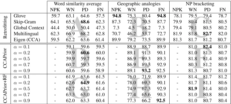
Table 1: Results for the word similarity datasets, geographic analogies and NP bracketing. The first upper blocks (A–C) present the results with retrofitting. NPK stands for no prior knowledge (no retrofitting is used), WN for WordNet, PD for PPDB and FN for FrameNet. Glove, Skip-Gram, Global Context, Multilingual and Eigen are the word embeddings of Pennington et al. (2014), Mikolov et al. (2013b), Huang et al. (2012), Faruqui and Dyer (2014) and Dhillon et al. (2015) respectively. The second middle blocks (D–F) show the results of our eigenword embeddings encoded with prior knowledge using our method. Each row in the block corresponds to a specific use of anαvalue (smoothing factor), as described in Figure 3. In the lower blocks (G–I) we take the word embeddings from the second block, and retrofit them using the method of Faruqui et al. (2015). Best results in each block are in bold.
art word embeddings, such as Glove (Pennington et al., 2014), Skip-Gram (Mikolov et al., 2013b), Global Context (Huang et al., 2012) and Multilin-gual (Faruqui and Dyer, 2014). We also compare our word embeddings with the Eigen word embeddings of Dhillon et al. (2015) without any prior knowl-edge.
Retrofitting for Prior Knowledge We compare
our approach of incorporating prior knowledge into the derivation of CCA against the previous works where prior knowledge is introduced in the off-the-shelf embeddings as a post-processing step (Faruqui et al., 2015; Rothe and Sch¨utze, 2015). In this pa-per, we focus on the retrofitting approach of Faruqui et al. (2015).
Retrofitting works by optimizing an objective function which has two terms: one that tries to keep the distance between the word vectors close to the original distances, and the other which enforces the vectors of words which are adjacent in the prior knowledge graph to be close to each other in the new
embedding space. We use the retrofitting package7 to compare our results in different settings against the results of retrofitting of Faruqui et al. (2015).
5.3 Evaluation Benchmarks
We evaluated the quality of our eigenword embed-dings on three different tasks: word similarity, geo-graphic analogies and NP bracketing.
Word Similarity For the word similarity task we
experimented with 11 different widely used bench-marks. The WS-353-ALL dataset (Finkelstein et al., 2002) consists of 353 pairs of English words with their human similarity ratings. Later, Agirre et al. (2009) re-annotated WS-353-ALL for similarity (WS-353-SIM) and relatedness (WS-353-REL) with specific distinctions between them. The SimLex-999 dataset (Hill et al., 2015) was built to measure how well models capture similarity, rather than relat-edness or association. The MEN-TR-3000 dataset (Bruni et al., 2014) consists of 3000 word pairs
7https://github.com/mfaruqui/
sampled from words that occur at least 700 times in a large web corpus. The datasets, MTurk-287 (Radinsky et al., 2011) and MTurk-771 (Halawi et al., 2012), were scored by Amazon Mechanical Turk workers for relatedness of English word pairs. The YP-130 (Yang and Powers, 2005) and Verb-143 (Baker et al., 2014) datasets were developed for verb similarity predictions. The last two datasets, MC-30 (Miller and Charles, 1991) and RG-65 (Rubenstein and Goodenough, 1965) consist of 30 and 65 noun pairs respectively.
For each dataset, we calculate the cosine similar-ity between the vectors of word pairs and measure Spearman’s rank correlation coefficient between the scores produced by the embeddings and human rat-ings. We report the average of the correlations on all 11 datasets. Each word similarity task in the above list represents a different aspect of word similarity, and as such, averaging the results points to the qual-ity of the word embeddings on several tasks. We later analyze specific datasets.
Geographic Analogies Mikolov et al. (2013c)
created a test set of analogous word pairs such as a:b c:draising the analogy question of the form “a is tobascis to ” wheredis unknown. We report results on a subset of this dataset which focuses on finding capitals of common countries, e.g., Greece
is toAthens as Iraq is to . This dataset consists of 506 word pairs. For given word pairs, a:b c:d wheredis unknown, we use the vector offset method (Mikolov et al., 2013b), i.e., we compute a vector v = vb −va+vc where va, vb and vc are vector
representations of the wordsa,bandcrespectively; we then return the word dwith the greatest cosine similarity tov.
NP Bracketing Here the goal is to identify the
correct bracketing of a three-word noun (Lazaridou et al., 2013). For example, the bracketing ofannual
(price growth)is “right,” while the bracketing of
(en-try level) machineis “left.” Similarly to Faruqui and
Dyer (2015), we concatenate the word vectors of the three words, and use this vector for binary classifi-cation into left or right.
Since most of the datasets that we evaluate on in this paper are not standardly separated into develop-ment and test sets, we report all results we calculated (with respect to hyperparameter differences) and do
not select just a subset of the results.
5.4 Evaluation
Preliminary Experiments In our first set of
ex-periments, we vary the dimension of the word em-bedding vectors. We try m ∈ {50,100,200,300}.
Our experiments showed that the results consistently improve when the dimension increases for all the different datasets. For example, for m = 50 and
WIKI1, we get an average of46.4on the word
sim-ilarity tasks,50.1form = 100, 53.4form = 200
and54.2form= 300. The more data are available,
the more likely larger dimension will improve the quality of the word embeddings. Indeed, for WIKI5,
we get an average of49.4, 54.9, 57.0 and59.5for
each of the dimensions. The improvements with re-spect to the dimension are consistent across all of our results, so we fixmat300.
We also noticed a consistent improvement in ac-curacy when using more data from Wikipedia. For example, for m = 300, using WIKI1 gives an
av-erage of54.1, while using WIKI2 gives an average
of54.9and finally, using WIKI5 gives an average of
59.5. We fix the dataset we use to be WIKI5.
Results Table 1 describes the results from our first
set of experiments. (Note that the table is divided into 9 distinct blocks, labeled A through I.) In gen-eral, adding prior knowledge to eigenword embed-dings does improve the quality of word vectors for the word similarity, geographic analogies and NP bracketing tasks on several occasions (blocks D–F compared to last row in blocks A–C). For example, our eigenword vectors encoded with prior knowl-edge (CCAPrior) consistently perform better than the eigenword vectors that do not have any prior knowledge for the word similarity task (59.5, Eigen
in the first row under NPK column, versus block D). The only exceptions are for α = 0.1 with Word-Net (59.1), for α = 0.7with PPDB (59.3) and for
α= 0.9with FrameNet (58.9), whereαdenotes the smoothing factor.
knowl-edge often performs better for word similarity and NP bracketing tasks (block D versus G and block F versus I). Interestingly, CCAPrior+RF embeddings also often perform better than eigenword vectors (Eigen) of Dhillon et al. (2015) when retrofitted using the method of Faruqui et al. (2015). For example, in the word similarity task, eigenwords retrofitted with WordNet get an accuracy of 62.2
whereas encoding prior knowledge using both CCA and retrofitting gets a maximum accuracy of 63.3. We see the same pattern for PPDB, with 63.6 for
“Eigen” and64.9for “CCAPrior+RF”. We
hypoth-esize that the reason for these changes is that the two methods for encoding prior knowledge maxi-mize different objective functions.
The performance with FrameNet is weaker, in some cases leading to worse performance (e.g., with Glove and SG vectors). We believe that FrameNet does not perform as well as the other lexicons be-cause it groups words based on very abstract con-cepts; often words with seemingly distantly related meanings (e.g., push and growth) can evoke the same frame. This also supports the findings of Faruqui et al. (2015), who noticed that the use of FrameNet as a prior knowledge resource for improv-ing the quality of word embeddimprov-ings is not as helpful as other resources such as WordNet and PPDB.
We note that CCA works especially well for the geographic analogies dataset. The quality of eigen-word embeddings (and the other embeddings) de-grades when we encode prior knowledge using the method of Faruqui et al. (2015). Our method im-proves the quality of eigenword embeddings.
Global Picture of the Results When comparing
retrofitting to CCA with prior knowledge, there is a noticable difference. Retrofitting performs well or badly, depending on the dataset, while the re-sults with CCA are more stable. We attribute this to the difference between how our algorithm and retrofitting work. Retrofitting makes adirectuse of the source of prior knowledge, by adding a regular-ization term that enforces words which are similar according to the prior knowledge to be closer in the embedding space. Our algorithm, on the other hand, makes a more indirect use of the source of prior knowledge, by changing the co-occurence matrix on which we do singular value decomposition.
Specifically, we believe that our algorithm is more stable to cases in which words for the task at hand are unknown words with respect to the source of prior knowledge. This is demonstrated with the ge-ographical analogies task: in that case, retrofitting lowers the results in most cases. The city and coun-try names do not appear in the sources of prior knowledge we used.
Further Analysis We further inspected the results
on the word similarity tasks for the RG-65 and WS-353-ALL datasets. Our goal was to find cases in which either CCA embeddings by themselves out-perform other types of embeddings or that encoding prior knowledge into CCA the way we describe sig-nificantly improves the results.
For the WS-353-ALL dataset, the eigenword em-beddings get a correlation of 69.6. The next best performing word embeddings are the multilingual word embeddings (68.0) and skip-gram (58.3). In-terestingly enough, the multilingual word embed-dings also use CCA to project words into a low-dimensional space using a linear transformation, suggesting that linear projections are a good fit for the WS-353-ALL dataset. The dataset itself includes pairs of common words with a corresponding simi-larity score. The words that appear in the dataset are actually expected to occur in similar contexts, a property that CCA directly encodes when deriving word embeddings.
The best performance on the RG-65 dataset is with the Glove word embeddings (76.6). CCA em-beddings give an accuracy of 69.7 on that dataset. However, with this dataset, we observe significant improvement when encoding prior knowledge using our method. For example, using WordNet with this dataset improves the results by 4.2 points (73.9). Us-ing the method of Faruqui et al. (2015) (with Word-Net) on top of our CCA word embeddings improves the results even further by 8.7 points (78.4).
The Role of Prior Knowledge We also designed
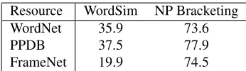
Resource WordSim NP Bracketing WordNet 35.9 73.6
PPDB 37.5 77.9
FrameNet 19.9 74.5
Table 2: Results on word similarity dataset (average over 11 datasets) and NP bracketing. The word embed-dings are derived by using SVD on the similarity graph extracted from the prior knowledge source (WordNet, PPDB and FrameNet).
that graph, and get embeddings of size 300. Table 2 gives the results when using these embeddings. We see that the results are consistently lower than the results that appear in Table 1, implying that the use of prior knowledge comes hand in hand with the use of distributional information. When using the retrofitting method by Faruqui et al. on top of these word embeddings, the results barely improved.
6 Related Work
Our ideas in this paper for encoding prior knowl-edge in eigenword embeddings relate to three main threads in existing literature.
One of the threads focuses on modifying the ob-jective of word vector training algorithms. Yu and Dredze (2014), Xu et al. (2014), Fried and Duh (2015) and Bian et al. (2014) augment the training objective in neural language models of Mikolov et al. (2013a) to encourage semantically related word vectors to come closer to each other. Wang et al. (2014) propose a method for jointly embedding en-tities (from FreeBase, a large community-curated knowledge base) and words (from Wikipedia) into the same continuous vector space. Chen and de Melo (2015) propose a similar joint model to im-prove the word embeddings, but rather than us-ing structured knowledge sources their model fo-cuses on discovering stronger semantic connections in specific contexts in a text corpus.
Another research thread relies on post-processing steps to encode prior knowledge from semantic lex-icons in off-the-shelf word embeddings. The main intuition behind this trend is to update word vec-tors by running belief propagation on a graph ex-tracted from the relation information in semantic lexicons. The retrofitting approach of Faruqui et al. (2015) uses such techniques to obtain higher
quality semantic vectors using WordNet, FrameNet, and the Paraphrase Database. They report on how retrofitting helps improve the performance of vari-ous off-the-shelf word vectors such as Glove, Skip-Gram, Global Context, and Multilingual, on vari-ous word similarity tasks. Rothe and Sch¨utze (2015) also describe how standard word vectors can be ex-tended to various data types in semantic lexicons, e.g., synsets and lexemes in WordNet.
Most of the standard word vector training algo-rithms use co-occurrence within window-based con-texts to measure relatedness among words. Sev-eral studies question the limitations of defining re-latedness in this way and investigate if the word co-occurrence matrix can be constructed to encode prior knowledge directly to improve the quality of word vectors. Wang et al. (2015) investigate the no-tion of relatedness in embedding models by incor-porating syntactic and lexicographic knowledge. In spectral learning, Yih et al. (2012) augment the word co-occurrence matrix on which LSA operates with relational information such that synonyms will tend to have positive cosine similarity, and antonyms will tend to have negative similarities. Their vector space representation successfully projects synonyms and antonyms on opposite sides in the projected space. Chang et al. (2013) further generalize this approach to encode multiple relations (and not just opposing relations, such as synonyms and antonyms) using multi-relational LSA.
In spectral learning, most of the studies on in-corporating prior knowledge in word vectors focus on LSA based word embeddings (Yih et al., 2012; Chang et al., 2013; Turney and Littman, 2005; Tur-ney, 2006; Turney and Pantel, 2010).
From the technical perspective, our work is also related to that of Jagarlamudi et al. (2011), who showed how to generalize CCA so that it uses lo-cality preserving projections (He and Niyogi, 2004). They also assume the existence of a weight matrix in a multi-view setting that describes the distances between pairs of points in the two views.
[image:11.612.98.271.53.103.2]7 Conclusion
We described a method for incorporating prior knowledge into CCA. Our method requires a rela-tively simple change to the original canonical cor-relation analysis, where extra counts are added to the matrix on which singular value decomposition is performed. We used our method to derive word em-beddings in the style of eigenwords, and tested them on a set of datasets. Our results demonstrate several advantages of encoding prior knowledge into eigen-word embeddings.
Acknowledgements
The authors would like to thank Paramveer Dhillon for his help with running theSWELLpackage. The authors would also like to thank Manaal Faruqui and Sujay Kumar Jauhar for their help and techni-cal assistance with the retrofitting package and the word embedding evaluation suite. Thanks also to Ankur Parikh for early discusions on this project. This work was completed while the first author was an intern at the University of Edinburgh, as part of the Equate Scotland program. This research was supported by an EPSRC grant (EP/L02411X/1) and an EU H2020 grant (688139/H2020-ICT-2015; SUMMA).
Appendix A: Proofs
Proof of Lemma 1. The proof is similar to the one that appears in Koren and Carmel (2003) for Lemma 3.1. The only difference is the use of two views. Note that
[X>LY]
ij =Pk,k0XkiLkk0Yk0j. As such,
[X>LY]ij= X
k,k0
(nδkk0−1)XkiYk0j
=
n X
k=1
nXkiYkj− n X
k=1 Xki
!
| {z } 0
× n X
k0=1 Yk0j
!
| {z } 0
=n[X>Y]ij,
whereδkk0 = 1iffk=k0 and0otherwise, and the
sec-ond equality relies on the assumption of the data being centered.
Proof of Lemma 2. Without loss of generality, assume d ≤ d0. Letu0
1, . . . , u0d be the left singular vectors of A andv0
1, . . . , vd00 be the right ones, and σ1, . . . , σd be
the singular values. ThereforeA=Pdj=1σju0j(v0j)>. In
addition, the objective equals (after substitutingA):
m X i=1 d X j=1
σjhui, u0jihvi, v0ji= d X j=1 σj m X i=1
hui, u0jihvi, vj0i !
(5)
Note that by the Cauchy-Schwartz inequality:
d X j=1 m X i=1
hui, u0jihvi, vj0i= m X i=1 d X j=1
hui, u0jihvi, vj0i
≤ m X i=1 v u u t d X j=1
|hui, u0ji|2 v u u t d X j=1
|hvi, v0ji|2≤m
In addition, note that if we chooseui =u0iandvi = vi0, then the inequality above becomes an equality, and
in addition, the objective in Eq. 5 will equal the sum of the m largest singular vectorsPmj=1σj. As such, this
assignment touiandvimaximizes the objective. Proof of Lemma 3. First, by definition of matrix multi-plication,
m X
k=1
(Xuk)>L(Y vk) = X i,j Lij m X k=1
[Xuk]i[Y vk]j !
.
(6)
Also,
dmij 2 = 1 2 m X k=1
[Xuk]2i −2[Xuk]i[Y vk]j+ [Y vk]2j !
.
Therefore,
2X
i,j
−Lij dmij 2
=X
i,j −Lij
m X
k=1
−2[Xuk]i[Y vk]j !
+X
i,j −Lij
m X
k=1
[Xuk]2i + [Y vk]2j !
| {z }
0
= 2X
i,j Lij
m X
k=1
[Xuk]i[Y vk]j, !
(7)
References
Eneko Agirre, Enrique Alfonseca, Keith Hall, Jana Kravalova, Marius Pas¸ca, and Aitor Soroa. 2009. A study on similarity and relatedness using distribu-tional and wordnet-based approaches. InProceedings of HLT-NAACL.
Francis Bach and Michael Jordan. 2005. A probabilistic interpretation of canonical correlation analysis. Tech Report 688, Department of Statistics, University of California, Berkeley.
Collin F. Baker, Charles J. Fillmore, and John B. Lowe. 1998. The Berkeley FrameNet project. In Proceed-ings of ACL.
Simon Baker, Roi Reichart, and Anna Korhonen. 2014. An unsupervised model for instance level subcatego-rization acquisition. InProceedings of EMNLP. Mohit Bansal, Kevin Gimpel, and Karen Livescu. 2014.
Tailoring continuous word representations for depen-dency parsing. InProceedings of ACL.
Mikhail Belkin, Partha Niyogi, and Vikas Sindhwani. 2006. Manifold regularization: A geometric frame-work for learning from labeled and unlabeled exam-ples.Journal of Machine Learning Research, 7:2399– 2434.
Yoshua Bengio, R´ejean Ducharme, Pascal Vincent, and Christian Janvin. 2003. A neural probabilistic lan-guage model.Journal of Machine Learning Research, 3:1137–1155.
Jiang Bian, Bin Gao, and Tie-Yan Liu. 2014. Knowledge-powered deep learning for word embed-ding. InMachine Learning and Knowledge Discovery in Databases, volume 8724 ofLecture Notes in Com-puter Science, pages 132–148.
Avrim Blum and Tom Mitchell. 1998. Combining la-beled and unlala-beled data with co-training. In Proceed-ings of COLT.
Elia Bruni, Nam-Khanh Tran, and Marco Baroni. 2014. Multimodal distributional semantics. Journal of Arti-ficial Intelligence Research, 49:1–47.
Kai-Wei Chang, Wen-tau Yih, and Christopher Meek. 2013. Multi-relational latent semantic analysis. In
Proceedings of EMNLP.
Jiaqiang Chen and Gerard de Melo. 2015. Semantic in-formation extraction for improved word embeddings. InProceedings of NAACL Workshop on Vector Space Modeling for NLP.
Shay B. Cohen, K. Stratos, Michael Collins, Dean P. Fos-ter, and Lyle Ungar. 2014. Spectral learning of latent-variable PCFGs: Algorithms and sample complexity.
Journal of Machine Learning Research.
Ronan Collobert and Jason Weston. 2008. A unified ar-chitecture for natural language processing: Deep neu-ral networks with multitask learning. InProceedings of ICML.
Scott Deerwester, Susan T. Dumais, George W. Furnas, Thomas K. Landauer, and Richard Harshman. 1990. Indexing by latent semantic analysis. Journal of the American Society for Information Science, 41(6):391– 407.
Paramveer S. Dhillon, Dean P. Foster, and Lyle H. Ungar. 2015. Eigenwords: Spectral word embeddings. Jour-nal of Machine Learning Research, 16:3035–3078. Manaal Faruqui and Chris Dyer. 2014. Improving vector
space word representations using multilingual correla-tion. InProceedings of EACL.
Manaal Faruqui and Chris Dyer. 2015. Non-distributional word vector representations. In Pro-ceedings of ACL.
Manaal Faruqui, Jesse Dodge, Sujay K. Jauhar, Chris Dyer, Eduard Hovy, and Noah A. Smith. 2015. Retrofitting word vectors to semantic lexicons. In Pro-ceedings of NAACL.
Lev Finkelstein, Gabrilovich Evgenly, Matias Yossi, Rivlin Ehud, Solan Zach, Wolfman Gadi, and Ruppin Eytan. 2002. Placing search in context: The concept revisited. ACM Transactions on Information Systems, 20(1):116–131.
Daniel Fried and Kevin Duh. 2015. Incorporating both distributional and relational semantics in word repre-sentations. InProceedings of ICLR.
Juri Ganitkevitch, Benjamin Van Durme, and Chris Callison-Burch. 2013. PPDB: The paraphrase database. InProceedings of NAACL.
Guy Halawi, Gideon Dror, Evgeniy Gabrilovich, and Yehuda Koren. 2012. Large-scale learning of word relatedness with constraints. InProceedings of ACM SIGKDD.
Zellig S. Harris. 1957. Co-occurrence and transforma-tion in linguistic structure.Language, 33(3):283–340. Xiaofei He and Partha Niyogi. 2004. Locality preserving
projections. InProceedings of NIPS.
Felix Hill, Roi Reichart, and Anna Korhonen. 2015. SimLex-999: Evaluating semantic models with (gen-uine) similarity estimation. Computational Linguis-tics, 41(4):665–695.
Eric H Huang, Richard Socher, Christopher D Manning, and Andrew Y Ng. 2012. Improving word representa-tions via global context and multiple word prototypes. InProceedings of ACL.
Jagadeesh Jagarlamudi and Hal Daum´e. 2012. Regu-larized interlingual projections: Evaluation on mul-tilingual transliteration. In Proceedings of EMNLP-CoNLL.
Yehuda Koren and Liran Carmel. 2003. Visualization of labeled data using linear transformations. In Proceed-ings of IEEE Conference on Information Visualization. Thomas K. Landauer, Peter W. Foltz, and Darrell La-ham. 1998. An introduction to latent semantic analy-sis.Discourse Processes, 25:259–284.
Angeliki Lazaridou, Eva Maria Vecchi, and Marco Ba-roni. 2013. Fish transporters and miracle homes: How compositional distributional semantics can help NP parsing. InProceedings of EMNLP.
Tomas Mikolov, Kai Chen, Greg Corrado, and Jeffrey Dean. 2013a. Efficient estimation of word represen-tations in vector space. InProceedings of ICLR Work-shop.
Tomas Mikolov, Ilya Sutskever, Kai Chen, Greg S Cor-rado, and Jeff Dean. 2013b. Distributed representa-tions of words and phrases and their compositionality. InProceedings of NIPS.
Tomas Mikolov, Wen tau Yih, and Geoffrey Zweig. 2013c. Linguistic regularities in continuous space word representations. InProceedings of NAACL-HLT. George A. Miller and Walter G. Charles. 1991. Contex-tual correlates of semantic similarity. Language and Cognitive Processes, 6(1):1–28.
George A Miller. 1995. WordNet: A lexical database for English. Communications of the ACM, 38(11):39–41. Andriy Mnih and Geoffrey Hinton. 2007. Three new graphical models for statistical language modelling. In
Proceedings of ICML.
Shashi Narayan and Shay B. Cohen. 2016. Optimizing spectral learning for parsing. InProceedings of ACL. Ankur P. Parikh, Shay B. Cohen, and Eric Xing. 2014.
Spectral unsupervised parsing with additive tree met-rics. InProceedings of ACL.
Jeffrey Pennington, Richard Socher, and Christopher Manning. 2014. Glove: Global vectors for word rep-resentation. InProceedings of EMNLP.
Kira Radinsky, Eugene Agichtein, Evgeniy Gabrilovich, and Shaul Markovitch. 2011. A word at a time: Com-puting word relatedness using temporal semantic anal-ysis. InProceedings of ACM WWW.
Sascha Rothe and Hinrich Sch¨utze. 2015. AutoEx-tend: Extending word embeddings to embeddings for synsets and lexemes. InProceedings of ACL-IJCNLP. Herbert Rubenstein and John B. Goodenough. 1965. Contextual correlates of synonymy. Communications of the ACM, 8(10):627–633.
Carina Silberer, Vittorio Ferrari, and Mirella Lapata. 2013. Models of semantic representation with visual attributes. InProceedings of ACL.
Richard Socher, John Bauer, Christopher D. Manning, and Andrew Y. Ng. 2013. Parsing with compositional vector grammars. InProceedings of ACL.
Karl Stratos, Michael Collins, and Daniel Hsu. 2015. Model-based word embeddings from decompositions of count matrices. InProceedings of ACL.
Karl Stratos, Michael Collins, and Daniel Hsu. 2016. Unsupervised part-of-speech tagging with anchor hid-den markov models. Transactions of the Association for Computational Linguistics, 4:245–257.
Peter D. Turney and Michael L. Littman. 2005. Corpus-based learning of analogies and semantic relations.
Machine Learning, 60(1-3):251–278.
Peter D. Turney and Patrick Pantel. 2010. From fre-quency to meaning: Vector space models of semantics.
Journal of Artificial Intelligence Research, 37(1):141– 188.
Peter D. Turney. 2006. Similarity of semantic relations.
Computational Linguistics, 32(3):379–416.
Zhen Wang, Jianwen Zhang, Jianlin Feng, and Zheng Chen. 2014. Knowledge graph and text jointly em-bedding. InProceedings of EMNLP.
Tong Wang, Abdelrahman Mohamed, and Graeme Hirst. 2015. Learning lexical embeddings with syntactic and lexicographic knowledge. In Proceedings of ACL-IJCNLP.
Chang Xu, Yalong Bai, Jiang Bian, Bin Gao, Gang Wang, Xiaoguang Liu, and Tie-Yan Liu. 2014. RC-NET: A general framework for incorporating knowledge into word representations. In Proceedings of the ACM CIKM.
Dongqiang Yang and David MW Powers. 2005. Mea-suring semantic similarity in the taxonomy of Word-Net. InProceedings of the Australasian Conference on Computer Science.
David Yarowsky. 1995. Unsupervised word sense dis-ambiguation rivaling supervised methods. In Proceed-ings of ACL.
Wen-tau Yih, Geoffrey Zweig, and John Platt. 2012. Po-larity inducing latent semantic analysis. In Proceed-ings of EMNLP-CoNLL.