Grouping Language Model Boundary Words to Speed
K
–Best Extraction
from Hypergraphs
Kenneth Heafield∗,† Philipp Koehn∗ Alon Lavie† ∗
School of Informatics University of Edinburgh
10 Crichton Street Edinburgh EH8 9AB, UK [email protected]
†
Language Technologies Institute Carnegie Mellon University
5000 Forbes Avenue Pittsburgh, PA 15213, USA {heafield,alavie}@cs.cmu.edu
Abstract
We propose a new algorithm to approximately extract top-scoring hypotheses from a hyper-graph when the score includes an N–gram language model. In the popular cube prun-ing algorithm, every hypothesis is annotated with boundary words and permitted to recom-bine only if all boundary words are equal. However, many hypotheses share some, but not all, boundary words. We use these com-mon boundary words to group hypotheses and do so recursively, resulting in a tree of hy-potheses. This tree forms the basis for our new search algorithm that iteratively refines groups of boundary words on demand. Ma-chine translation experiments show our algo-rithm makes translation 1.50 to 3.51 times as fast as with cube pruning in common cases.
1 Introduction
This work presents a new algorithm to search a packed data structure for high-scoring hypothe-ses when the score includes an N–gram language model. Many natural language processing systems have this sort of problem e.g. hypergraph search in hierarchical and syntactic machine translation (Mi et al., 2008; Klein and Manning, 2001), lat-tice rescoring in speech recognition, and confusion network decoding in optical character recognition (Tong and Evans, 1996). Large language models have been shown to improve quality, especially in machine translation (Brants et al., 2007; Koehn and Haddow, 2012). However, language models make search computationally expensive because they ex-amine surface words without regard to the structure
at North Korea in North Korea with North Korea with the DPRK
at
North Korea in
with
the DPRK
Figure 1: Hypotheses are grouped by common prefixes and suffixes.
of the packed search space. Prior work, including cube pruning (Chiang, 2007), has largely treated the language model as a black box. Our new search algorithm groups hypotheses by common prefixes and suffixes, exploiting the tendency of the language model to score these hypotheses similarly. An exam-ple is shown in Figure 1. The result is a substantial improvement over the time-accuracy trade-off pre-sented by cube pruning.
The search spaces mentioned in the previous para-graph are special cases of a directed acyclic hyper-graph. As used here, the difference from a nor-mal graph is that an edge can go from one vertex to any number of vertices; this number is thearity
of the edge. Lattices and confusion networks are hypergraphs in which every edge happens to have arity one. We experiment with parsing-based ma-chine translation, where edges represent grammar rules that may have any number of non-terminals, including zero.
Hypotheses are paths in the hypergraph scored by a linear combination of features. Many features are
additive: they can be expressed as weights on edges that sum to form hypothesis features. However, log probability from anN–gram language model is
additive because it examines surface strings across edge and vertex boundaries. Non-additivity makes search difficult because locally optimal hypotheses may not be globally optimal.
In order to properly compute the language model score, each hypothesis is annotated with its bound-ary words, collectively referred to as its state (Li and Khudanpur, 2008). Hypotheses with equal state may be recombined, so a straightforward dynamic programming approach (Bar-Hillel et al., 1964) sim-ply treats state as an additional dimension in the dy-namic programming table. However, this approach quickly becomes intractable for large language mod-els where the number of states is too large.
Beam search (Chiang, 2005; Lowerre, 1976) ap-proximates the straightforward algorithm by remem-bering abeamof up tokhypotheses1in each vertex. It visits each vertex in bottom-up order, each time calling abeam filling algorithmto selectk hypothe-ses. The parameterk is a time-accuracy trade-off: largerkincreases both CPU time and accuracy.
We contribute a new beam filling algorithm that improves the time-accuracy trade-off over the popu-lar cube pruning algorithm (Chiang, 2007) discussed in§2.3. The algorithm is based on the observation that competing hypotheses come from the same im-put, so their language model states are often similar. Grouping hypotheses by these similar words enables our algorithm to reason over multiple hypotheses at once. The algorithm is fully described in§3.
2 Related Work
2.1 Alternatives to Bottom-Up Search
Beam search visits each vertex in the hypergraph in bottom-up (topological) order. The hypergraph can also be searched in left-to-right order (Watanabe et al., 2006; Huang and Mi, 2010). Alternatively, hypotheses can be generated on demand with cube growing (Huang and Chiang, 2007), though we note that it showed little improvement in Moses (Xu and Koehn, 2012). All of these options are compatible with our algorithm. However, we only experiment with bottom-up beam search.
1We useKto denote the number of fully-formed hypotheses requested by the user andkto denote beam size.
2.2 Exhaustive Beam Filling
Originally, beam search was used with an exhaustive beam filling algorithm (Chiang, 2005). It generates every possible hypothesis (subject to the beams in previous vertices), selects the top k by score, and discards the remaining hypotheses. This is expen-sive: just one edge of arity a encodes O(1 +ak) hypotheses and each edge is evaluated exhaustively. In the worst case, our algorithm is exhaustive and generates the same number of hypotheses as beam search; in practice, we are concerned with the aver-age case.
2.3 Baseline: Cube Pruning
Cube pruning (Chiang, 2007) is a fast approximate beam filling algorithm and our baseline. It chooses
khypotheses by popping them off the top of a prior-ity queue. Initially, the queue is populated with hy-potheses made from the best (highest-scoring) parts. These parts are an edge and a hypothesis from each vertex referenced by the edge. When a hypothesis is popped, several next-best alternatives are pushed. These alternatives substitute the next-best edge or a next-best hypothesis from one of the vertices.
Our work follows a similar pattern of popping one queue entry then pushing multiple entries. However, our queue entries are a group of hypotheses while cube pruning’s entries are a single hypothesis.
Hypotheses are usually fully scored before being placed in the priority queue. An alternative priori-tizes hypotheses by theiradditive score. The addi-tive score is the edge’s score plus the score of each component hypothesis, ignoring the non-additive as-pect of the language model. When the additive score is used, the language model is only calledktimes, once for each hypothesis popped from the queue.
Cube pruning can produce duplicate queue en-tries. Gesmundo and Henderson (2010) modified the algorithm prevent duplicates instead of using a hash table. We include their work in the experiments.
2.4 Exact Algorithms
A number of exact search algorithms have been de-veloped. We are not aware of an exact algorithm that tractably scales to the size of hypergraphs and lan-guage models used in many modern machine trans-lation systems (Callison-Burch et al., 2012).
The hypergraph and language model can be com-piled into an integer linear program. The best hy-pothesis can then be recovered by taking the dual and solving by Lagrangian relaxation (Rush and Collins, 2011). However, that work only dealt with language models up to order three.
Iglesias et al. (2011) represent the search space as a recursive transition network and the language model as a weighted finite state transducer. Using standard finite state algorithms, they intersect the two automatons then exactly search for the highest-scoring paths. However, the intersected automaton is too large. The authors suggested removing low probability entries from the language model, but this form of pruning negatively impacts translation qual-ity (Moore and Quirk, 2009; Chelba et al., 2010). Their work bears some similarity to our algorithm in that partially overlapping state will be collapsed and efficiently handled together. However, the key advatage to our approach is that groups have a score that can be used for pruningbeforethe group is ex-panded, enabling pruning without first constructing the intersected automaton.
2.5 Coarse-to-Fine
Coarse-to-fine (Petrov et al., 2008) performs mul-tiple pruning passes, each time with more detail. Search is a subroutine of coarse-to-fine and our work is inside search, so the two are compatible. There are several forms of coarse-to-fine search; the closest to our work increases the language model order each iteration. However, by operating inside search, our algorithm is able to handle hypotheses at different levels of refinement and use scores to choose where to further refine hypotheses. Coarse-to-fine decod-ing cannot do this because it determines the level of refinement before calling search.
3 Our New Beam Filling Algorithm
In our algorithm, the primary idea is to group hy-potheses with similar language model state. The
following sections formalize what these groups are (partial state), that the groups have a recursive struc-ture (state tree), how groups are split (bread crumbs), using groups with hypergraph edges (partial edge), prioritizing search (scoring) and best-first search (priority queue).
3.1 Partial State
An N–gram language model (with orderN) com-putes the probability of a word given theN−1 pre-ceding words. The left state of a hypothesis is the first N −1 words, which have insufficient context to be scored. Right state is the lastN −1 words; these might become context for another hypothesis. Collectively, they are known as state. State mini-mization (Li and Khudanpur, 2008) may reduce the size of state due to backoff in the language model.
For example, the hypothesis “the few nations that have diplomatic relations with North Korea” might have left state “the few” and right state “Korea” after state minimization determined that “North” could be elided. Collectively, the state is denoted (the fewa `Korea). The diamondis a stand-in for elided words. Terminatorsaand`indicate when left and right state are exhausted, respectively2.
Our algorithm is based on partial state. Par-tial state is simply state with more inner words elided. For example, (theKorea) is a partial state for (the fewa `Korea). Terminatorsaand`can be elided just like words. Empty state is denoted using the customary symbol for empty string,. For example, () is the empty partial state. The termi-nators serve to distinguish a completed state (which may be short due to state minimization) from an in-complete partial state.
3.2 State Tree
States (the fewa `Korea) and (thea `Korea) have words in common, so the partial state (theKorea) can be used to reason over both of them. Generalizing this notion to the set of hypothe-ses in a beam, we build a state tree. The root of the tree is the empty partial state () that reasons
2
A corner case arises for hypotheses with less thanN −1
()
(a) (aKorea) (aa Korea)
(aa `Korea)
(aa in Korea) (aa `in Korea) (some) (someDPRK) (somea DPRK) (somea `DPRK)
(the) (theKorea)
(thea Korea) (thea `Korea)
[image:4.612.90.522.58.176.2](the fewKorea) (the few `Korea) (the fewa `Korea)
Figure 2: A state tree containing five states: (the fewa `Korea), (thea `Korea), (somea `DPRK), (aa `in Korea), and (aa `Korea). Nodes of the tree are partial states. The branching order is the first word, the last word, the second word, and so on. If the left or right state is exhausted, then branching continues with the remaining state. For purposes of branching, termination symbolsaand`act like normal words.
()
(aa Korea)
(aa `Korea) (aa `in Korea) (somea `DPRK) (theKorea)
[image:4.612.334.519.255.377.2](thea `Korea) (the fewa `Korea)
Figure 3: The optimized version of Figure 2. Nodes immediately reveal the longest shared prefix and suffix among hypotheses below them.
over all hypotheses. From the root, the tree branches by the first word of state, the last word, the second word, the second-to-last word, and so on. If left or right state is exhausted, then branching continues us-ing the remainus-ing state. The branchus-ing order priori-tizes the outermost words because these can be used to update the language model probability. The deci-sion to start with left state is arbitrary. An example tree is shown in Figure 2.
As an optimization, each node determines the longest shared prefix and suffix of the hypotheses below it. The node reports these words immedi-ately, rendering some other nodes redundant. This makes our algorithm faster because it will then only encounter nodes when there is a branching decision to be made. The original tree is shown in Figure 2 and the optimized version is shown in Figure 3. As a side effect of branching by left state first, the al-gorithm did not notice that states (theKorea) and
()[1+]
(aa Korea)
(aa `Korea) (aa `in Korea) (somea `DPRK)
(theKorea)
(thea `Korea) (the fewa `Korea)
(theKorea)[0+]
(thea `Korea) (the fewa `Korea)
Figure 4: Visiting the root node partitions the tree into best child (theKorea)[0+] and bread crumb ()[1+].
The data structure remains intact for use elsewhere.
(aa Korea) both end with Korea. We designed the tree building algorithm for speed and plan to exper-iment with alternatives as future work.
The state tree is built lazily. A node initially holds a flat array of all the hypotheses below it. When its children are first needed, the hypotheses are grouped by the branching word and an array of child nodes is built. In turn, these newly created children each initially hold an array of hypotheses. CPU time is saved because nodes containing low-scoring nodes may never construct their children.
[image:4.612.104.267.256.377.2]3.3 Bread Crumbs
The state tree is explored in a best-first manner. Specifically, when the algorithm visits a node, it considers that node’s best child. The best child re-veals more words, so the score may go up or down when the language model is consulted. Therefore, simply following best children may lead to a poor hypothesis. Some backtracking mechanism is re-quired, for which we use bread crumbs. Visiting a node results in two items: the best child and a bread crumb. The bread crumb encodes the node that was visited and how many children have already been considered. Figure 4 shows an example.
More formally, each node has an array of chil-dren sorted by score, so it suffices for the bread crumb to keep an index in this array. An in-dex of zero denotes that no child has been vis-ited. Continuing the example from Figure 3, ()[0+] denotes the root partial state with chil-dren starting at index 0 (i.e. all of them). Visit-ing ()[0+] yields best child (theKorea)[0+] and bread crumb ()[1+]. Later, the search al-gorithm may return to ()[1+], yielding best child (somea `DPRK)[0+] and bread crumb ()[2+]. If there is no remaining sibling, visit-ing yields only the best child.
The index serves to restrict the array of children to those with that index or above. Formally, let d
map from a node or bread crumb to the set of leaves descended from it. The descendants of a nodenare those of its children
d(n) = |n|−1
G
i=0
d(n[i])
wherettakes the union of disjoint sets and n[i]is theith child. In a bread crumb with indexc, only de-scendents by the remaining children are considered
d(n[c+]) = |n|−1
G
i=c
d(n[i])
It follows that the set of descendants ispartitioned
into two disjoint sets
d(n[c+]) =d(n[c])Gd(n[c+ 1+])
3.4 Partial Edge
The beam filling algorithm is tasked with selecting hypotheses given a number of hypergraph edges. Hypergraph edges are strings comprised of words and references to vertices (in parsing, terminals and non-terminals). A hypergraph edge is converted to a
partial edgeby replacing each vertex reference with the root node from that vertex. For example, the hy-pergraph edge “isv.” referencing vertexvbecomes partial edge “is ()[0+] .”
Partial edges allow our algorithm to reason over a large set of hypotheses at once. Visiting a partial edge divides that set into two as follows. A heuristic chooses one of the non-leaf nodes to visit. Currently, this heuristic picks the node with the fewest words revealed. As a tie breaker, it chooses the leftmost node. The chosen node is visited (partitioned), yielding the best child and bread crumb as described in the previous section. These are substituted into separate copies of the par-tial edge. Continuing our example with the vertex shown in Figure 3, “is ()[0+] .” partitions into “is (theKorea)[0+] .” and “is ()[1+] .”
3.5 Scoring
Every partial edge has a score that determines its search priority. Initially, this score is the sum of the edge’s score and the scores of each bread crumb (de-fined below). As words are revealed, the score is updated to account for new language model context. Each edge score includes a log language model probability and possibly additive features. When-ever there is insufficient context to compute the lan-guage model probability of a word, an estimateris used. For example, edge “isv.” incorporates esti-mate
logr(is)r(.)
into its score. The same applies to hypotheses: (the fewa `Korea) includes estimate
logr(the)r(few|the)
because the words in left state are those with insuf-ficient context.
Kneser-Ney smoothing (Kneser and Ney, 1995) to assume that backoff has occurred. An alternative is to use average-case rest costs explicitly stored in the language model (Heafield et al., 2012). Both options are used in the experiments3.
The score of a bread crumb is the maximum score of its descendants as defined in§3.3. For example, the bread crumb ()[1+] has a lower score than ()[0+] because the best child (theKorea)[0+] and its descendants no longer contribute to the max-imum.
The score of partial edge “is ()[0+] .” is the sum of scores from its two parts: edge “isv.” and bread crumb ()[0+]. The edge’s score includes estimated log probability logr(is)r(.)as explained earlier. The bread crumb’s score comes from its highest-scoring descendent (the fewa `Korea) and therefore includes esti-matelogr(the)r(few|the).
Estimates are updated as words are revealed. Continuing the example, “is ()[0+] .” has best child “is (theKorea)[0+] .” In this best child, the estimater(.) is updated to r(.|Korea). Similarly,
r(the) is replaced withr(the|is). Updates exam-ine only words that have been revealed:r(few|the) remains unrevised.
Updates are computed efficiently by using point-ers (Heafield et al., 2011) with KenLM. To summa-rize, the language model computes
r(wn|wn1−1)
r(wn|wni−1)
in a single call. In the popular reverse trie data struc-ture, the language model visitswni while retrieving
wn1, so the cost is the same as a single query. More-over, when the language model earlier provided es-timater(wn|wni−1), it also returned a data-structure pointer t(wni). Pointers are retained in hypotheses, edges, and partial edges for each word with an esti-mated probability. When context is revealed, our al-gorithm queries the language model with new con-text wi1−1 and pointert(win). The language model uses this pointer to immediately retrieve denomina-torr(wn|wni−1)and as a starting point to retrieve nu-meratorr(wn|wn1−1). It can therefore avoid looking
3
We also tested upper bounds (Huang et al., 2012; Carter et al., 2012) but the result is still approximate due to beam pruning and initial experiments showed degraded performance.
up r(wn), r(wn|wn−1), . . . , r(wn|wni+1−1) as would normally be required with a reverse trie.
3.6 Priority Queue
Our beam filling algorithm is controlled by a priority queue containing partial edges. The queue is popu-lated by converting all outgoing hypergraph edges into partial edges and pushing them onto the queue. After this initialization, the algorithm loops. Each iteration begins by popping the top-scoring partial edge off the queue. If all nodes are leaves, then the partial edge is converted to a hypothesis and placed in the beam. Otherwise, the partial edge is parti-tioned as described in§3.3. The two resulting partial edges are pushed onto the queue. Looping continues with the next iteration until the queue is empty or the beam is full. After the loop terminates, the beam is given to the root node of the state tree; other nodes will be built lazily as described in§3.2.
Overall, the algorithm visits hypergraph vertices in bottom-up order. Our beam filling algorithm runs in each vertex, making use of state trees in vertices below. The top of the tree contains full hypotheses. If a K-best list is desired, packing and extraction works the same way as with cube pruning.
4 Experiments
Performance is measured by translating the 3003-sentence German-English test set from the 2011 Workshop on Machine Translation (Callison-Burch et al., 2011). Two translation models were built, one hierarchical (Chiang, 2007) and one with target syn-tax. The target-syntax system is based on English parses from the Collins (1999) parser. Both were trained on Europarl (Koehn, 2005). The language model interpolates models built on Europarl, news commentary, and news data provided by the evalua-tion. Interpolation weights were tuned on the 2010 test set. Language models were built with SRILM (Stolcke, 2002), modified Kneser-Ney smoothing (Kneser and Ney, 1995; Chen and Goodman, 1998), default pruning, and order 5. Feature weights were tuned with MERT (Och, 2003), beam size 1000, 100-best output, and cube pruning. Systems were built with the Moses (Hoang et al., 2009) pipeline.
-101.6 -101.5 -101.4
0 1 2
A
v
erage
model
score
[image:7.612.86.539.63.286.2]CPU seconds/sentence This work Additive cube pruning Cube pruning
Figure 5: Hierarchial system in Moses with our algo-rithm, cube pruning with additive scores, and cube prun-ing with full scores (§2.3). The two baselines overlap.
relevant files were forced into the operating system disk cache before each run. CPU time is the to-tal user and system time taken by the decoder mi-nus loading time. Loading time was measured by running the decoder with empty input. In partic-ular, CPU time includes the cost of parsing. Our test system has 32 cores and 64 GB of RAM; no run came close to running out of memory. While multi-threaded experiments showed improvements as well, we only report single-threaded results to re-duce noise and to compare with cdec (Dyer et al., 2010). Decoders were compiled with the optimiza-tion settings suggested in their documentaoptimiza-tion.
Search accuracy is measured by average model score; higher is better. Only relative comparisons are meaningful because model scores have arbitrary scale and include constant factors. Beam sizes start at 5 and rise until a time limit determined by running the slowest algorithm with beam size 1000.
[image:7.612.312.543.65.283.2]4.1 Comparison Inside Moses
Figure 5 shows Moses performance with this work and with cube pruning. These results used the hi-erarchical system with common-practice estimates (§3.5). The two cube pruning variants are explained in§2.3. Briefly, the queue can be prioritized using
-101.6 -101.5 -101.4
0 1 2
A
v
erage
model
score
CPU seconds/sentence This work Gesmundo 1 Gesmundo 2 Cube pruning
Figure 6: Hierarchical system in cdec with our algorithm, similarly-performing variants of cube pruning defined in Gesmundo and Henderson (2010), and the default.
additive or full scores. Performance with additive scores is roughly the same as using full scores with half the beam size.
Our algorithm is faster for every beam size tested. It is also more accurate than additive cube pruning with the same beam size. However, when compared with full scores cube pruning, it is less accurate for beam sizes below 300. This makes sense because our algorithm starts with additive estimates and iter-atively refines them by calling the language model. Moreover, when beams are small, there are fewer chances to group hypotheses. With beams larger than 300, our algorithm can group more hypotheses, overtaking both forms of cube pruning.
Accuracy improvements can be interpreted as speed improvements by asking how much time each algorithm takes to achieve a set level of accuracy. By this metric, our algorithm is 2.04 to 3.37 times as fast as both baselines.
4.2 Comparison Inside cdec
[image:7.612.80.303.65.284.2]-101.6 -101.5 -101.4
0 1 2
A
v
erage
model
score
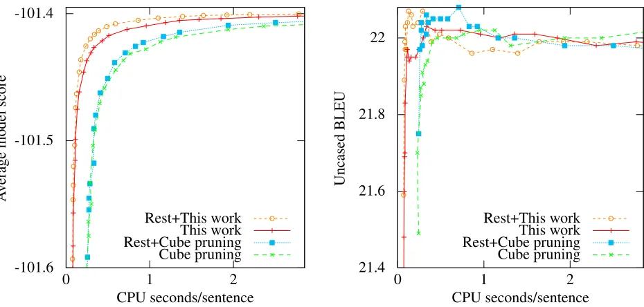
CPU seconds/sentence Rest+This work
This work Rest+Cube pruning Cube pruning
21.4 21.6 21.8 22
0 1 2
Uncased
BLEU
CPU seconds/sentence Rest+This work
[image:8.612.79.544.63.285.2]This work Rest+Cube pruning Cube pruning
Figure 7: Effect of rest costs on our algorithm and on cube pruning in Moses. Noisy BLEU scores reflect model errors.
are comparable with Moses4.
Measuring at equal accuracy, our algorithm makes cdec 1.56 to 2.24 times as fast as the best baseline. At first, this seems to suggest that cdec is faster. In fact, the opposite is true: comparing Fig-ures 5 and 6 reveals that cdec has a higher parsing cost than Moses5, thereby biasing the speed ratio to-wards 1. In subsequent experiments, we use Moses because it more accurately reflects search costs.
4.3 Average-Case Rest Costs
Previous experiments used the common-practice probability estimate described in §3.5. Figure 7 shows the impact of average-case rest costs on our algorithm and on cube pruning in Moses. We also looked at uncased BLEU (Papineni et al., 2002) scores, finding that our algorithm attains near-peak BLEU in less time. The relationship between model score and BLEU is noisy due to model errors.
4The glue rule builds hypotheses left-to-right. In Moses, glued hypotheses start with<s>and thus have empty left state. In cdec, sentence boundary tokens are normally added last, so intermediate hypotheses have spurious left state. Running cdec with the Moses glue rule led to improved time-accuracy perfor-mance. The improved version is used in all results reported. We accounted for constant-factor differences in feature definition i.e. whether<s>is part of the word count.
5In-memory phrase tables were used with both decoders. The on-disk phrase table makes Moses slower than cdec.
Average-case rest costs impact our algorithm more than they impact cube pruning. For small beam sizes, our algorithm becomes more accurate, mostly eliminating the disadvantage reported in§4.1. Com-pared to the common-practice estimate with beam size 1000, rest costs made our algorithm 1.62 times as fast and cube pruning 1.22 times as fast.
Table 1 compares our best result with the best baseline: our algorithm and cube pruning, both with rest costs inside Moses. In this scenario, our algo-rithm is 2.59 to 3.51 times as fast as cube pruning.
4.4 Target-Syntax
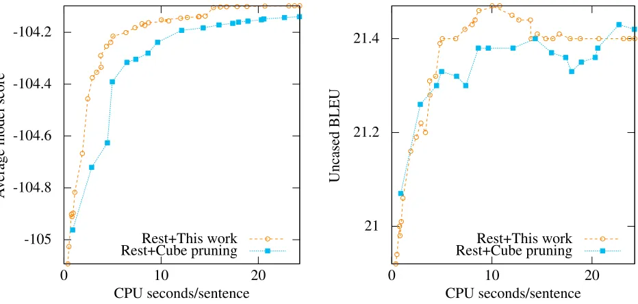
We took the best baseline and best result from previ-ous experiments (Moses with rest costs) and ran the target-syntax system. Results are shown in Figure 8. Parsing and search are far more expensive. For beam size 5, our algorithm attains equivalent accu-racy 1.16 times as fast. Above 5, our algorithm is 1.50 to 2.00 times as fast as cube pruning. More-over, our algorithm took less time with beam size 6900 than cube pruning took with beam size 1000.
-105 -104.8 -104.6 -104.4 -104.2
0 10 20
A
v
erage
model
score
CPU seconds/sentence Rest+This work Rest+Cube pruning
21 21.2 21.4
0 10 20
Uncased
BLEU
[image:9.612.80.546.64.286.2]CPU seconds/sentence Rest+This work Rest+Cube pruning
Figure 8: Performance of Moses with the target-syntax system.
extracted due to reordering. An appropriate prepo-sitional phrase (PP) was pruned with smaller beam sizes because it is disfluent.
4.5 Memory
Peak virtual memory usage was measured before each process terminated. Compared with cube prun-ing at a beam size of 1000, our algorithm uses 160 MB more RAM in Moses and 298 MB less RAM in cdec. The differences are smaller with lower beam sizes and minor relative to 12-13 GB total size, most of which is the phrase table and language model.
Rest+This work Rest+Cube pruning k CPU Model BLEU CPU Model BLEU
5 0.068 -1.698 21.59 0.243 -1.667 21.75 10 0.076 -1.593 21.89 0.255 -1.592 21.97 50 0.125 -1.463 22.07 0.353 -1.480 22.04 75 0.157 -1.446 22.06 0.408 -1.462 22.05 100 0.176 -1.436 22.03 0.496 -1.451 22.05 500 0.589 -1.408 22.00 1.356 -1.415 22.00 750 0.861 -1.405 21.96 1.937 -1.409 21.98 1000 1.099 -1.403 21.97 2.502 -1.407 21.98
Table 1: Numerical results from the hierarchical system for select beam sizeskcomparing our best result with the best baseline, both in Moses with rest costs enabled. To conserve space, model scores are shown with 100 added.
5 Conclusion
We have described a new search algorithm that achieves equivalent accuracy 1.16 to 3.51 times as fast as cube pruning, including two implementations and four variants. The algorithm is based on group-ing similar language model feature states together and dynamically expanding these groups. In do-ing so, it exploits the language model’s ability to estimate with incomplete information. Our imple-mentation is available under the LGPL as a stand-alone from http://kheafield.com/code/
and distributed with Moses and cdec.
Acknowledgements
[image:9.612.73.297.514.649.2]References
Yehoshua Bar-Hillel, Micha Perles, and Eli Shamir. 1964. On Formal Properties of Simple Phrase Struc-ture Grammars. Hebrew University Students’ Press. Thorsten Brants, Ashok C. Popat, Peng Xu, Franz J.
Och, and Jeffrey Dean. 2007. Large language mod-els in machine translation. InProceedings of the 2007 Joint Conference on Empirical Methods in Natural Language Processing and Computational Language Learning, pages 858–867, June.
Chris Callison-Burch, Philipp Koehn, Christof Monz, and Omar Zaidan. 2011. Findings of the 2011 work-shop on statistical machine translation. InProceedings of the Sixth Workshop on Statistical Machine Transla-tion, pages 22–64, Edinburgh, Scotland, July. Associ-ation for ComputAssoci-ational Linguistics.
Chris Callison-Burch, Philipp Koehn, Christof Monz, Matt Post, Radu Soricut, and Lucia Specia. 2012. Findings of the 2012 workshop on statistical machine translation. In Proceedings of the Seventh Work-shop on Statistical Machine Translation, pages 10– 51, Montr´eal, Canada, June. Association for Compu-tational Linguistics.
Simon Carter, Marc Dymetman, and Guillaume Bouchard. 2012. Exact sampling and decoding in high-order hidden Markov models. In Proceedings of the 2012 Joint Conference on Empirical Methods in Natural Language Processing and Computational Natural Language Learning, pages 1125–1134, Jeju Island, Korea, July.
Ciprian Chelba, Thorsten Brants, Will Neveitt, and Peng Xu. 2010. Study on interaction between entropy prun-ing and Kneser-Ney smoothprun-ing. InProceedings of In-terspeech, pages 2242–2245.
Stanley Chen and Joshua Goodman. 1998. An empirical study of smoothing techniques for language modeling. Technical Report TR-10-98, Harvard University, Au-gust.
David Chiang. 2005. A hierarchical phrase-based model for statistical machine translation. In Proceedings of the 43rd Annual Meeting on Association for Computa-tional Linguistics, pages 263–270, Ann Arbor, Michi-gan, June.
David Chiang. 2007. Hierarchical phrase-based transla-tion. Computational Linguistics, 33:201–228, June. Michael Collins. 1999. Head-Driven Statistical Models
for Natural Language Parsing. Ph.D. thesis, Univer-sity of Pennsylvania.
Chris Dyer, Adam Lopez, Juri Ganitkevitch, Johnathan Weese, Ferhan Ture, Phil Blunsom, Hendra Setiawan, Vladimir Eidelman, and Philip Resnik. 2010. cdec: A decoder, alignment, and learning framework for finite-state and context-free translation models. In
Proceedings of the ACL 2010 System Demonstrations, ACLDemos ’10, pages 7–12.
Andrea Gesmundo and James Henderson. 2010. Faster cube pruning. In Proceedings of the International Workshop on Spoken Language Translation (IWSLT), pages 267–274.
Peter Hart, Nils Nilsson, and Bertram Raphael. 1968. A formal basis for the heuristic determination of mini-mum cost paths. IEEE Transactions on Systems Sci-ence and Cybernetics, 4(2):100–107, July.
Kenneth Heafield, Hieu Hoang, Philipp Koehn, Tetsuo Kiso, and Marcello Federico. 2011. Left language model state for syntactic machine translation. In Pro-ceedings of the International Workshop on Spoken Language Translation, San Francisco, CA, USA, De-cember.
Kenneth Heafield, Philipp Koehn, and Alon Lavie. 2012. Language model rest costs and space-efficient storage. In Proceedings of the 2012 Joint Conference on Em-pirical Methods in Natural Language Processing and Computational Natural Language Learning, Jeju Is-land, Korea.
Hieu Hoang, Philipp Koehn, and Adam Lopez. 2009. A unified framework for phrase-based, hierarchical, and syntax-based statistical machine translation. In
Proceedings of the International Workshop on Spoken Language Translation, pages 152–159, Tokyo, Japan. Mark Hopkins and Greg Langmead. 2009. Cube pruning
as heuristic search. InProceedings of the 2009 Confer-ence on Empirical Methods in Natural Language Pro-cessing, pages 62–71, Singapore, August.
Liang Huang and David Chiang. 2007. Forest rescoring: Faster decoding with integrated language models. In
Proceedings of the 45th Annual Meeting of the Asso-ciation for Computational Linguistics, Prague, Czech Republic.
Liang Huang and Haitao Mi. 2010. Efficient incremental decoding for tree-to-string translation. InProceedings of the 2010 Conference on Empirical Methods in Natu-ral Language Processing, pages 273–283, Cambridge, MA, October.
Zhiheng Huang, Yi Chang, Bo Long, Jean-Francois Cre-spo, Anlei Dong, Sathiya Keerthi, and Su-Lin Wu. 2012. Iterative Viterbi A* algorithm for k-best se-quential decoding. In Proceedings of the 2012 Joint Conference on Empirical Methods in Natural guage Processing and Computational Natural Lan-guage Learning, pages 1125–1134, Jeju Island, Korea, July.
Natural Language Processing, pages 1373–1383, Ed-inburgh, Scotland, UK, July. Association for Compu-tational Linguistics.
Dan Klein and Christopher D. Manning. 2001. Parsing and hypergraphs. InProceedings of the Seventh Inter-national Workshop on Parsing Technologies, Beijing, China, October.
Reinhard Kneser and Hermann Ney. 1995. Improved backing-off for m-gram language modeling. In Pro-ceedings of the IEEE International Conference on Acoustics, Speech and Signal Processing, pages 181– 184.
Philipp Koehn and Barry Haddow. 2012. Towards effective use of training data in statistical machine translation. InProceedings of the Seventh Workshop on Statistical Machine Translation, pages 317–321, Montr´eal, Canada, June. Association for Computa-tional Linguistics.
Philipp Koehn. 2005. Europarl: A parallel corpus for statistical machine translation. InProceedings of MT Summit.
Zhifei Li and Sanjeev Khudanpur. 2008. A scalable decoder for parsing-based machine translation with equivalent language model state maintenance. In Pro-ceedings of the Second ACL Workshop on Syntax and Structure in Statistical Translation (SSST-2), pages 10–18, Columbus, Ohio, June.
Bruce Lowerre. 1976. The Harpy Speech Recognition System. Ph.D. thesis, Carnegie Mellon University. Haitao Mi, Liang Huang, and Qun Liu. 2008.
Forest-based translation. In Proceedings of ACL-08: HLT, pages 192–199, Columbus, Ohio, June.
Robert C. Moore and Chris Quirk. 2009. Less is more: Significance-based n-gram selection for smaller, better language models. InProceedings of the 2009 Confer-ence on Empirical Methods in Natural Language Pro-cessing, pages 746–755, August.
Franz Josef Och. 2003. Minimum error rate training in statistical machine translation. In ACL ’03: Pro-ceedings of the 41st Annual Meeting on Association for Computational Linguistics, pages 160–167, Mor-ristown, NJ, USA. Association for Computational Lin-guistics.
Kishore Papineni, Salim Roukos, Todd Ward, and Wei-Jing Zhu. 2002. BLEU: A method for automatic evalution of machine translation. InProceedings 40th Annual Meeting of the Association for Computational Linguistics, pages 311–318, Philadelphia, PA, July. Slav Petrov, Aria Haghighi, and Dan Klein. 2008.
Coarse-to-fine syntactic machine translation using lan-guage projections. InProceedings of the 2008 Confer-ence on Empirical Methods in Natural Language Pro-cessing, pages 108–116, Honolulu, HI, USA, October.
Alexander Rush and Michael Collins. 2011. Exact decoding of syntactic translation models through la-grangian relaxation. InProceedings of the 49th An-nual Meeting of the Association for Computational Linguistics, pages 72–82, Portland, Oregon, USA, June.
Andreas Stolcke. 2002. SRILM - an extensible language modeling toolkit. InProceedings of the Seventh Inter-national Conference on Spoken Language Processing, pages 901–904.
Xiang Tong and David A. Evans. 1996. A statistical approach to automatic OCR error correction in con-text. InProceedings of the Fourth Workshop on Very Large Corpora, pages 88–100, Copenhagen, Den-mark, April.
Taro Watanabe, Hajime Tsukada, and Hideki Isozaki. 2006. Left-to-right target generation for hierarchical phrase-based translation. In Proceedings of the 21st International Conference on Computational Linguis-tics and 44th Annual Meeting of the ACL, pages 777– 784, Sydney, Australia, July.