KLUE: Simple and robust methods for polarity classification
Thomas Proisl and Paul Greiner and Stefan Evert and Besim Kabashi Friedrich-Alexander-Universität Erlangen-Nürnberg
Department Germanistik und Komparatistik Professur für Korpuslinguistik
Bismarckstr. 6 91054 Erlangen, Germany
{thomas.proisl,paul.greiner,stefan.evert,besim.kabashi}@fau.de
Abstract
This paper describes our approach to the SemEval-2013 task on “Sentiment Analysis in Twitter”. We use simple bag-of-words mod-els, a freely available sentiment dictionary auto-matically extended with distributionally similar terms, as well as lists of emoticons and inter-net slang abbreviations in conjunction with fast and robust machine learning algorithms. The resulting system is resource-lean, making it rel-atively independent of a specific language. De-spite its simplicity, the system achieves compet-itive accuracies of 0.70–0.72 in detecting the sentiment of text messages. We also apply our approach to the task of detecting the context-dependent sentiment of individual words and phrases within a message.
1 Introduction
The SemEval-2013 task on “Sentiment Analysis in Twitter” (Wilson et al., 2013) focuses on polarity clas-sification, i. e. the problem of determining whether a textual unit, e. g. a document, paragraph, sentence or phrase, expresses a positive, negative or neutral sentiment (for a review of research topics and re-cent developments in the field of sentiment analysis see Liu (2012)). There are two subtasks: in task B, “Message Polarity Classification”, whole messages have to be classified as being of positive, negative or neutral sentiment; in task A, “Contextual Polarity Disambiguation”, a marked instance of a word or phrase has to be classified in the context of a whole message.
The training data for task B consist of approxi-mately 10 200 manually annotated Twitter messages,
the training data for task A of approximately 9 500 marked instances in approximately 6 300 Twitter mes-sages.1 The test data consist of in-domain Twit-ter messages (3 813 messages for task B and 4 435 marked instances in 2 826 messages for task A) and out-of-domain SMS text messages (2 094 messages for task B, 2 334 marked instances in 1 437 messages for task A). The distribution of messages and marked instances over sentiment categories in the training and test sets is shown in Tab. 1.
pos neg neu total
train-B 3 783 1 600 4 832 10 215
test-B Twitter 1 572 601 1 640 3 813
test-B SMS 492 394 1 208 2 094
train-A 5 862 3 166 463 9 491
test-A Twitter 2 734 1 541 160 4 435
test-A SMS 1 071 1 104 159 2 334
Table 1: The data sets for both tasks
The main focus of the current paper lies on experi-menting with resource-lean and robust methods for task B, the classification of whole messages. We do, however, apply our approach also to task A.
2 Features used for polarity classification
Our general approach is quite simple: we extract feature vectors from the training data (based on the
1These figures indicate the amount of training data we were actually able to use. Due to Twitter’s licensing conditions, the training data could only be made available as a collection of IDs. Even when using the official Twitter API for collecting the actual messages rather than the screen-scraping approach suggested by the task organizers, ca. 10% of the data were not (or no longer) available.
original messages and a small number of additional resources) and feed them into fast and robust super-vised machine learning algorithms implemented in the Python machine learning library scikit-learn (Pe-dregosa et al., 2011). For task B, the features are computed on the basis of the whole message; for task A, we use essentially the same features, but compute them once for the marked word or phrase and once for the rest of the message. All the features we use are described in some more detail in the following subsections.
2.1 Bag of words
We experimented with three different sets of bag-of-words features: unigrams, unigrams and bigrams, and an extended unigram model that includes a simple treatment of negation. For all three models we simply use the word frequencies as feature weights.
Our preprocessing pipeline starts with a simple preliminary tokenization step (lowercasing the whole message and splitting it on whitespace). In the re-sulting list of tokens, all user IDs and web URLs are replaced with placeholders.2 Any remaining punctu-ation is stripped from the tokens and empty tokens are deleted. In the extended unigram model, up to three tokens following a negation marker are then prefixed withnot_(fewer tokens if another negation marker or the end of the message is reached). Finally all words are stemmed using the Snowball stemmer.3 For a token unigram or bigram to be included in the bag of words models, it has to occur in at least five messages.
As an additional feature we include the total num-ber of tokens per message.
2.2 Features based on a sentiment dictionary
Widely-used algorithms such as SentiStrength (Thel-wall et al., 2010) rely heavily on dictionaries contain-ing sentiment ratcontain-ings of words and/or phrases. We use features based on an extended version of AFINN-111 (Nielsen, 2011).4
The AFINN sentiment dictionary contains senti-ment ratings ranging from−5 (very negative) to 5
2The regular expression for matching web URLs has been taken from http://daringfireball.net/2010/07/ improved_regex_for_matching_urls.
3http://snowball.tartarus.org/
4http://www2.imm.dtu.dk/pubdb/p.php?6010
(very positive) for 2 476 word forms. In order to ob-tain a better coverage, we extended the dictionary with distributionally similar words. For this pur-pose, large-vocabulary distributional semantic mod-els (DSM) were constructed from a version of the English Wikipedia5and the Google Web 1T 5-Grams database (Brants and Franz, 2006). The Wikipedia DSM consists of 122 281 case-folded word forms as target terms and 30 484 mid-frequency content words (lemmatised) as feature terms; the Web1T5 DSM of 241 583 case-folded word forms as target terms and 100 063 case-folded word forms as fea-ture terms. Both DSMs use a context window of two words to the left and right, and were reduced to 300 latent dimensions using randomized singular value decomposition (Halko et al., 2009).
For each AFINN entry, the 30 nearest neighbours according to each DSM were considered as exten-sion candidates. Sentiment ratings for the new candi-dates were computed by averaging over the 30 near-est neighbours of the respective candidate term (with scores set to 0 for all neighbours not listed in AFINN), and rescaling to the range[−5,5].6 After some ini-tial experiments, only candidates with a computed rating≤ −2.5 or≥2.5 were retained, resulting in an extended dictionary of 2 820 word forms.
As with the bag of words model, we make use of a simple heuristic treatment of negation: following a negation marker, the polarity of the next sentiment-carrying token up to a distance of at most four tokens is multiplied by−1.
The sentiment dictionary is used to extract four features:I) the number of tokens that express a posi-tive sentiment,II) the number of tokens that express
a negative sentiment,III) the total number of tokens
that express a sentiment according to our sentiment dictionary andIV) the arithmetic mean of all the sen-timent scores from the sensen-timent dictionary in the message.
5We used the pre-processed and linguistically annotated Wackypedia corpus available from http://wacky.sslmit. unibo.it/.
2.3 Features based on emoticons and internet slang abbreviations
In addition to the sentiment dictionary we use a list of 212 emoticons and 95 internet slang abbreviations from Wikipedia. We manually classified these 307 emotion markers as negative (−1), neutral (0) or pos-itive (1).
The extracted features based on this list are similar to the ones based on the sentiment dictionary. We use
I) the number of positive emotion markers,II) the number of negative emotion markers,III) the total number of emotion markers andIV) the arithmetic mean of all the emotion markers in the message.
3 Experiments
In this section we evaluate different classifiers (multi-nomial Naive Bayes,7Linear SVM8and Maximum Entropy9) and various combinations of features on the gold test sets. We vary the bag-of-words model (bow), the use of AFINN (sent), our extensions to the sentiment dictionary (ext) and the list of emotion markers (emo). To present as clear a picture of the classifiers’ performances as possible, we report F-scores for each of the three classes, the weighted av-erage of all three F-scores (Fw), the (unweighted)
av-erage of the positive and negative F-scores (Fpos+neg;
this is the value shown in the official task results and used for ranking systems), as well as accuracy.
Results for submitted systems are typeset in italics, the best results in each column are typeset in bold font.
3.1 Task B: Message Polarity Classification
Experiments with just a simple unigram bag-of-words model show that for both the Twitter (Tab. 3) and the SMS data (Tab. 4) the Maximum Entropy classifier outperforms multinomial Naive Bayes and Linear SVM by a considerable margin. For compar-ison, we also include some weak baselines (Tab. 2). The random baselines classify messages randomly,10
7We always use the default settingalpha = 1.0.
8In all experiments, we use the following parameters:
penalty = ‘l1’, dual = False, C = 1.0.
9We use the following parameter settings in our experiments:
penalty = ‘l1’, C = 1.0. 10random
uniformassumes a uniform probability distribution (all categories have equal probabilities), randomweighted has learned the probability distribution from the training data,
the majority baselines simply assign all messages to the most frequent category in the training data.11 As one would expect, all three learning algorithms are vastly superior to those baselines. Using both unigrams and bigrams in the bag-of-words model improves classifier peformance; so does the extended unigram model with negations.
For the Twitter data, adding the sentiment dictio-nary, the dictionary extensions and the list of emo-tion markers further improves classifier performance, with the best results being achieved by a combina-tion of all these features with a uni- and bigram bag-of-words model. The best combination of features would have been the fourth best system out of 35 constrained systems (sixth best out of all 51 systems), one rank higher than our task submission.12
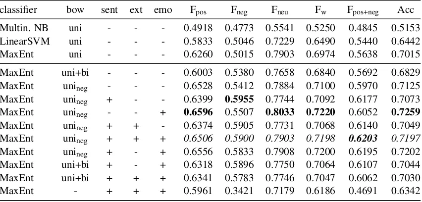
For the SMS data, adding the sentiment dictio-nary and the dictiodictio-nary extensions seems to improve the official score Fpos+neg, but slightly decreases
weighted average F-score and accuracy. This might be due to the greater orthographical variation in SMS texts. Emotion markers seem to be a much better sentiment indicator in the SMS data. But while just combining the list of emotion markers with the ex-tended unigram bag-of-words model leads to the best weighted average F-score and accuracy, Fpos+negis
best when a combination of all features is used. This is also the system we submitted, being the third best system (out of 44) for that task.
3.2 Task A: Contextual Polarity
Disambiguation
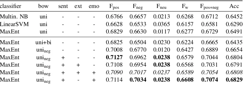
The results for task A are similar to those for task B in that Maximum Entropy is the best classifier for the unigram bag-of-words model for both the Twitter (Tab. 5) and the SMS data (Tab. 6). Adding negation treatment to the bag-of-words model increases classi-fier performance, as do the inclusion of AFINN and the use of emotion markers. Interestingly, extend-ing the sentiment dictionary based on distributional similarity leads to slightly worse results. Therefore,
randomweighted,binaryuses the same probability distribution but classifies messages only as either positive or negative.
11majority classifies all messages as neutral, as this is the most frequent category in the training data, majoritybinarydoes binary classification and thus classifies all messages as positive.
classifier Fpos Fneg Fneu Fw Fpos+neg Acc
randomuniform 0.3666 0.2128 0.3745 0.3458 0.2897 0.3318
randomweighted 0.3912 0.1681 0.4521 0.3820 0.2796 0.3835
randomweighted,binary 0.5186 0.2042 0.000 0.2460 0.3614 0.3349
majority 0.0000 0.0000 0.6015 0.2587 0.0000 0.4301
[image:4.612.96.520.210.413.2]majoritybinary 0.5838 0.0000 0.0000 0.2407 0.2919 0.4123
Table 2: Some weak baselines for task B, Twitter test set
classifier bow sent ext emo Fpos Fneg Fneu Fw Fpos+neg Acc
Multin. NB uni - - - 0.6355 0.5093 0.6898 0.6390 0.5724 0.6423
LinearSVM uni - - - 0.6412 0.4884 0.6876 0.6371 0.5648 0.6418
MaxEnt uni - - - 0.6705 0.5109 0.7212 0.6671 0.5907 0.6761
MaxEnt uni+bi - - - 0.6845 0.5192 0.7257 0.6762 0.6019 0.6845
MaxEnt unineg - - - 0.6797 0.5284 0.7242 0.6750 0.6041 0.6824
MaxEnt unineg + - - 0.6860 0.5661 0.7284 0.6854 0.6261 0.6911
MaxEnt unineg - - + 0.6807 0.5393 0.7229 0.6766 0.6100 0.6835
MaxEnt unineg + + - 0.6841 0.5529 0.7258 0.6814 0.6185 0.6874
MaxEnt unineg + + + 0.6963 0.5650 0.7325 0.6912 0.6306 0.6968
MaxEnt unineg + - + 0.6952 0.5753 0.7338 0.6929 0.6353 0.6984
MaxEnt uni+bi + - + 0.7034 0.5706 0.7358 0.6964 0.6370 0.7018
MaxEnt uni+bi + + + 0.7052 0.5720 0.7371 0.6979 0.6386 0.7031
MaxEnt - + + + 0.6920 0.3532 0.6533 0.6220 0.5226 0.6370
Table 3: Evaluation results for task B on the Twitter test set
classifier bow sent ext emo Fpos Fneg Fneu Fw Fpos+neg Acc
Multin. NB uni - - - 0.4918 0.4773 0.5541 0.5250 0.4845 0.5153
LinearSVM uni - - - 0.5833 0.5046 0.7229 0.6490 0.5440 0.6442
MaxEnt uni - - - 0.6260 0.5015 0.7903 0.6974 0.5638 0.7015
MaxEnt uni+bi - - - 0.6003 0.5380 0.7658 0.6840 0.5692 0.6829
MaxEnt unineg - - - 0.6528 0.5412 0.7884 0.7100 0.5970 0.7125
MaxEnt unineg + - - 0.6399 0.5955 0.7744 0.7092 0.6177 0.7073
MaxEnt unineg - - + 0.6596 0.5507 0.8033 0.7220 0.6052 0.7259
MaxEnt unineg + + - 0.6374 0.5905 0.7731 0.7068 0.6140 0.7049
MaxEnt unineg + + + 0.6506 0.5900 0.7903 0.7198 0.6203 0.7197
MaxEnt unineg + - + 0.6556 0.5833 0.7908 0.7200 0.6195 0.7202
MaxEnt uni+bi + - + 0.6318 0.5896 0.7750 0.7064 0.6107 0.7044
MaxEnt uni+bi + + + 0.6341 0.5783 0.7746 0.7047 0.6062 0.7030
MaxEnt - + + + 0.5961 0.3421 0.7179 0.6186 0.4691 0.6342
[image:4.612.94.520.462.666.2]classifier bow sent ext emo Fpos Fneg Fneu Fw Fpos+neg Acc
Multin. NB uni - - - 0.7799 0.6164 0.0498 0.6967 0.6981 0.7067
LinearSVM uni - - - 0.7759 0.6046 0.0576 0.6905 0.6902 0.6949
MaxEnt uni - - - 0.7974 0.6155 0.0110 0.7059 0.7065 0.7218
MaxEnt uni+bi - - - 0.8071 0.6320 0.0222 0.7179 0.7195 0.7335
MaxEnt unineg - - - 0.8058 0.6380 0.0110 0.7188 0.7219 0.7342
MaxEnt unineg + - - 0.8160 0.6610 0.0317 0.7339 0.7385 0.7479
MaxEnt unineg + + - 0.8153 0.6583 0.0316 0.7325 0.7368 0.7466
MaxEnt unineg + + + 0.8141 0.6608 0.0330 0.7326 0.7374 0.7468
MaxEnt unineg + - + 0.8153 0.6664 0.0331 0.7353 0.7409 0.7493
Table 5: Evaluation results for task A on the Twitter test set
classifier bow sent ext emo Fpos Fneg Fneu Fw Fpos+neg Acc
Multin. NB uni - - - 0.6766 0.6657 0.0213 0.6268 0.6712 0.6452
LinearSVM uni - - - 0.6628 0.6533 0.0365 0.6157 0.6581 0.6290
MaxEnt uni - - - 0.6829 0.6630 0.0117 0.6277 0.6729 0.6491
MaxEnt uni+bi - - - 0.6825 0.6504 0.0230 0.6224 0.6665 0.6435
MaxEnt unineg - - - 0.7008 0.6770 0.0120 0.6427 0.6889 0.6654
MaxEnt unineg + - - 0.7127 0.6962 0.0238 0.6579 0.7044 0.6804
MaxEnt unineg + + - 0.7108 0.6954 0.0238 0.6568 0.7031 0.6791
MaxEnt unineg + + + 0.7090 0.7017 0.0237 0.6589 0.7054 0.6808
[image:5.612.94.523.237.387.2]MaxEnt unineg + - + 0.7114 0.7034 0.0238 0.6608 0.7074 0.6829
Table 6: Evaluation results for task A on the SMS test set
we could have improved upon our task submission by excluding the sentiment dictionary extensions – however, the gains are very small and the system’s ranks would still be the same (17/28 for the Twitter data, 16/26 for the SMS data).
4 Discussion
4.1 Error analysis
4.1.1 Task B: Message Polarity Classification
The most prominent problem, according to the con-fusion matrix in Tab. 7, is that a lot of negative mes-sages are classified as neutral; the same problem exists to a lesser extent for positive messages.
A qualitative analysis of mis-classified messages for which the MaxEnt classifier indicated high con-fidence suggests that the human annotators did not clearly distinguish between sentiment expressed by the authors of messages and their own response to message content. For example, the messages shown
predicted
pos neg neu
gold
pos 979 352 70 40 523 100
neg 70 47 287 213 244 134
neu 191 191 58 75 1391 942
Table 7: Task B, confusion matrix for tweets/SMS
in (1) and (2) report a negative and positive event, respectively, in a neutral way and should therefore be annotated with neutral sentiment. However, in the test data they are labelled as negative and positive by the human annotators.
(2) European Exchanges open with a slight rise: (AGI) Rome, October 24 - Euro-pean Exchanges opened with a slight ris... http://t.co/mAljf6eT
This problem is probably a major factor in the mis-classification of many negative and positive messages as neutral. In order to better reproduce the human annotations, the system would additionally have to decide whether a reported event is of a negative, pos-itive or neutral natureper se– a quite different task that would require external training data and world knowledge.
An analysis of mis-classified positive messages further suggests that certain punctuation marks, espe-cially multiple exclamation marks, might be useful as additional features.
4.1.2 Task A: Contextual Polarity
Disambiguation
The confusion matrix in Tab. 8 shows that mes-sages marked as negative in the test data often mis-classified as positive and vice versa, while neutral instances are overwhelmingly classified as positive or negative. This suggests that for the classifiers we use, there might be too few neutral instances in the training data (cf. Tab. 1).
predicted
pos neg neu
gold
pos 2329 826 397 239 8 6
neg 550 341 980 761 11 2
[image:6.612.322.514.112.289.2]neu 109 92 48 65 3 2
Table 8: Task A, confusion matrix for tweets/SMS
4.2 Conclusion and future work
We use a resource-lean approach, relying only on three external resources: a stemmer, a relatively small sentiment dictionary and an even smaller list of emotion markers. Stemmers are already avail-able for many languages and both kinds of lexical resources can be gathered relatively easily for other languages. The list of emotion markers should apply to most languages. This makes our whole system rel-atively language-independent, provided that a similar amount of manually labelled training data is
avail-able.13 In fact, the learning curve for our system (Fig. 1) suggests that even as few as 3 000–3 500 labelled messages might be sufficient. The similar
0.0
0.2
0.4
0.6
0.8
1.0
Amount of training data
Score
500 1500 2500 3500 4500 5500 6500 7500 8500 9500 Fpos+neg Accuracy
Figure 1: Learning curve of our system for the “Message Polarity Classification” task, evaluated on the Twitter data
evaluation results for the Twitter and the SMS data show that not relying on Twitter-specific features like hashtags pays off: by making our system as generic as possible, it is robust, not overfitted to the training data, and generalizes well to other types of data. The methods discussed in the current paper are particu-larly well suited to the “Message Polarity Classifica-tion” task, our system ranking amongst the best. It turns out, however, that simply applying the same ap-proach to the “Contextual Polarity Disambiguation” task yields only mediocre results.
In the future, we would like to experiment with a couple of additional features. Determining the near-est neighbors of a message based on Latent Semantic Analysis might be a useful addition, as might be the use of part-of-speech tags created by an in-domain POS tagger (Gimpel et al., 2011)14. We would also like to find out whether a heuristic treatment of inten-sifiers and deteninten-sifiers, the normalization of character repetitions, or the inclusion of some punctuation-based features could further improve classifier per-formance.
13For task B, even the extended unigram bag-of-words model by itself, without any additional resources, would have per-formed quite well as the 9th best constrained system on the Twitter test set (13th best system overall) and the 5th best system on the SMS test set.
References
Thorsten Brants and Alex Franz. 2006. Web 1T 5-gram Version 1. Linguistic Data Consortium, Philadelphia, PA.
Kevin Gimpel, Nathan Schneider, Brendan O’Connor, Di-panjan Das, Daniel Mills, Jacob Eisenstein, Michael Heilman, Dani Yogatama, Jeffrey Flanigan, and Noah A. Smith. 2011. Part-of-speech tagging for Twitter: Annotation, features, and experiments. In Pro-ceedings of the 49th Annual Meeting of the Association for Computational Linguistics, pages 42–47, Portland, Oregon. Association for Computational Linguistics. N. Halko, P. G. Martinsson, and J. A. Tropp. 2009.
Find-ing structure with randomness: Stochastic algorithms for constructing approximate matrix decompositions. Technical Report 2009-05, ACM, California Institute of Technology, September.
Bing Liu. 2012.Sentiment Analysis and Opinion Mining. Synthesis Lectures on Human Language Technologies. Morgan & Claypool.
Finn Årup Nielsen. 2011. A new ANEW: Evaluation of a word list for sentiment analysis in microblogs. In
Proceedings of the ESWC2011 Workshop on ‘Making Sense of Microposts’: Big things come in small pack-ages, number 718 in CEUR Workshop Proceedings, pages 93–98, Heraklion.
F. Pedregosa, G. Varoquaux, A. Gramfort, V. Michel, B. Thirion, O. Grisel, M. Blondel, P. Prettenhofer, R. Weiss, V. Dubourg, J. Vanderplas, A. Passos, D. Cournapeau, M. Brucher, M. Perrot, and E. Duches-nay. 2011. Scikit-learn: Machine learning in Python.
Journal of Machine Learning Research, 12:2825–2830. Mike Thelwall, Kevan Buckley, Georgios Paltoglou, Di Cai, and Arvid Kappas. 2010. Sentiment in short strength detection informal text.Journal of the Amer-ican Society for Information Science and Technology, 61(12):2544–2558.