Shallow Parsing with Conditional Random Fields
Fei Sha
and
Fernando Pereira
Department of Computer and Information Science
University of Pennsylvania
200 South 33rd Street, Philadelphia, PA 19104
(feisha|pereira)@cis.upenn.edu
Abstract
Conditional random fields for sequence label-ing offer advantages over both generative mod-els like HMMs and classifiers applied at each sequence position. Among sequence labeling tasks in language processing, shallow parsing has received much attention, with the devel-opment of standard evaluation datasets and ex-tensive comparison among methods. We show here how to train a conditional random field to achieve performance as good as any reported base noun-phrase chunking method on the CoNLL task, and better than any reported sin-gle model. Improved training methods based on modern optimization algorithms were crit-ical in achieving these results. We present ex-tensive comparisons between models and train-ing methods that confirm and strengthen pre-vious results on shallow parsing and training methods for maximum-entropy models.
1 Introduction
Sequence analysis tasks in language and biology are of-ten described as mappings from input sequences to se-quences of labels encoding the analysis. In language pro-cessing, examples of such tasks include part-of-speech tagging, named-entity recognition, and the task we shall focus on here, shallow parsing. Shallow parsing iden-tifies the non-recursive cores of various phrase types in text, possibly as a precursor to full parsing or informa-tion extracinforma-tion (Abney, 1991). The paradigmatic shallow-parsing problem is NP chunking, which finds the non-recursive cores of noun phrases called base NPs. The pioneering work of Ramshaw and Marcus (1995) in-troduced NP chunking as a machine-learning problem, with standard datasets and evaluation metrics. The task was extended to additional phrase types for the CoNLL-2000 shared task (Tjong Kim Sang and Buchholz, CoNLL-2000),
which is now the standard evaluation task for shallow parsing.
Most previous work used two main machine-learning approaches to sequence labeling. The first approach re-lies onk-order generative probabilistic models of paired input sequences and label sequences, for instance hidden Markov models (HMMs) (Freitag and McCallum, 2000; Kupiec, 1992) or multilevel Markov models (Bikel et al., 1999). The second approach views the sequence labeling problem as a sequence of classification problems, one for each of the labels in the sequence. The classification re-sult at each position may depend on the whole input and on the previouskclassifications.1
The generative approach provides well-understood training and decoding algorithms for HMMs and more general graphical models. However, effective genera-tive models require stringent conditional independence assumptions. For instance, it is not practical to make the label at a given position depend on a window on the in-put sequence as well as the surrounding labels, since the inference problem for the corresponding graphical model would be intractable. Non-independent features of the inputs, such as capitalization, suffixes, and surrounding words, are important in dealing with words unseen in training, but they are difficult to represent in generative models.
The sequential classification approach can handle many correlated features, as demonstrated in work on maximum-entropy (McCallum et al., 2000; Ratnaparkhi, 1996) and a variety of other linear classifiers, including winnow (Punyakanok and Roth, 2001), AdaBoost (Ab-ney et al., 1999), and support-vector machines (Kudo and Matsumoto, 2001). Furthermore, they are trained to min-imize some function related to labeling error, leading to smaller error in practice if enough training data are avail-able. In contrast, generative models are trained to max-imize the joint probability of the training data, which is
1Ramshaw and Marcus (1995) used transformation-based learning (Brill, 1995), which for the present purposes can be tought of as a classification-based method.
not as closely tied to the accuracy metrics of interest if the actual data was not generated by the model, as is always the case in practice.
However, since sequential classifiers are trained to make the best local decision, unlike generative mod-els they cannot trade off decisions at different positions against each other. In other words, sequential classifiers are myopic about the impact of their current decision on later decisions (Bottou, 1991; Lafferty et al., 2001). This forced the best sequential classifier systems to re-sort to heuristic combinations of forward-moving and backward-moving sequential classifiers (Kudo and Mat-sumoto, 2001).
Conditional random fields (CRFs) bring together the best of generative and classification models. Like classi-fication models, they can accommodate many statistically correlated features of the inputs, and they are trained dis-criminatively. But like generative models, they can trade off decisions at different sequence positions to obtain a globally optimal labeling. Lafferty et al. (2001) showed that CRFs beat related classification models as well as HMMs on synthetic data and on a part-of-speech tagging task.
In the present work, we show that CRFs beat all re-ported single-model NP chunking results on the standard evaluation dataset, and are statistically indistinguishable from the previous best performer, a voting arrangement of 24 forward- and backward-looking support-vector clas-sifiers (Kudo and Matsumoto, 2001). To obtain these results, we had to abandon the original iterative scing CRF trainscing algorithm for convex optimization al-gorithms with better convergence properties. We provide detailed comparisons between training methods.
The generalized perceptron proposed by Collins (2002) is closely related to CRFs, but the best CRF train-ing methods seem to have a slight edge over the general-ized perceptron.
2 Conditional Random Fields
We focus here on conditional random fields on sequences, although the notion can be used more generally (Laf-ferty et al., 2001; Taskar et al., 2002). Such CRFs define conditional probability distributionsp(Y|X)of label se-quences given input sese-quences. We assume that the ran-dom variable sequencesXandY have the same length,
and usex=x1· · ·xn andy =y1· · ·ynfor the generic
input sequence and label sequence, respectively.
A CRF on(X,Y)is specified by a vectorf oflocal
featuresand a correspondingweight vectorλ. Each local
feature is either astate features(y,x, i)or atransition feature t(y, y0,x, i), where y, y0 are labels, xan input sequence, andian input position. To make the notation
more uniform, we also write
s(y, y0,x, i) = s(y0,x, i) s(y,x, i) = s(yi,x, i)
t(y,x, i) =
t(yi−1, yi,x, i) i >1
0 i= 1
for any state featuresand transition featuret. Typically, features depend on the inputs around the given position, although they may also depend on global properties of the input, or be non-zero only at some positions, for instance features that pick out the first or last labels.
The CRF’sglobal feature vectorfor input sequencex
and label sequenceyis given by
F(y,x) =X
i
f(y,x, i)
where i ranges over input positions. The conditional probability distribution defined by the CRF is then
pλ(Y|X) =expλ·F(Y,X)
Zλ(X) (1)
where
Zλ(x) =X y
expλ·F(y,x)
Any positive conditional distributionp(Y|X)that obeys theMarkov property
p(Yi|{Yj}j6=i,X) =p(Yi|Yi−1, Yi+1,X)
can be written in the form (1) for appropriate choice of feature functions and weight vector (Hammersley and Clifford, 1971).
The most probable label sequence for input sequence
xis
ˆ
y= arg max
y pλ(y|x) = arg maxy
λ·F(y,x)
becauseZλ(x)does not depend ony. F(y,x) decom-poses into a sum of terms for consecutive pairs of labels, so the most likelyycan be found with the Viterbi
algo-rithm.
We train a CRF by maximizing the log-likelihood of a given training setT ={(xk,yk)}Nk=1, which we assume fixed for the rest of this section:
Lλ = Pklogpλ(yk|xk)
= P
k[λ·F(yk,xk)−logZλ(xk)]
To perform this optimization, we seek the zero of the gra-dient
∇Lλ=
X
k
F(yk,xk)−Epλ(Y|xk)F(Y,xk)
In words, the maximum of the training data likelihood is reached when the empirical average of the global fea-ture vector equals its model expectation. The expectation Epλ(Y|x)F(Y,x) can be computed efficiently using a variant of the forward-backward algorithm. For a given
x, define thetransition matrixfor positionias
Mi[y, y0] = expλ·f(y, y0,x, i)
Let f be any local feature, fi[y, y0] = f(y, y0,x, i),
F(y,x) = P
if(yi−1, yi,x, i), and let ∗ denote
component-wise matrix product. Then
Epλ(Y|x)F(Y,x) =
X
y
pλ(y|x)F(y,x)
= X
i
αi−1(fi∗Mi)β>i
Zλ(x)
Zλ(x) = αn·1>
where αi and βi the forward and backward state-cost
vectors defined by
αi =
αi−1Mi 0< i≤n
1 i= 0
β>i =
Mi+1β>i+1 1≤i < n
1 i=n
Therefore, we can use a forward pass to compute theαi
and a backward bass to compute theβi and accumulate
the feature expectations.
To avoid overfitting, we penalize the likelihood with a spherical Gaussian weight prior (Chen and Rosenfeld, 1999):
L0λ=
X
k
[λ·F(yk,xk)−logZλ(xk)]
−kλk
2
2σ2 +const with gradient
∇L0 λ=
X
k
F(yk,xk)−Epλ(Y|xk)F(Y,xk)
− λ
σ2
3 Training Methods
Lafferty et al. (2001) used iterative scaling algorithms for CRF training, following earlier work on maximum-entropy models for natural language (Berger et al., 1996; Della Pietra et al., 1997). Those methods are very sim-ple and guaranteed to converge, but as Minka (2001) and Malouf (2002) showed for classification, their conver-gence is much slower than that of general-purpose convex
optimization algorithms when many correlated features are involved. Concurrently with the present work, Wal-lach (2002) tested conjugate gradient and second-order methods for CRF training, showing significant training speed advantages over iterative scaling on a small shal-low parsing problem. Our work shows that precon-ditioned conjugate-gradient (CG) (Shewchuk, 1994) or limited-memory quasi-Newton (L-BFGS) (Nocedal and Wright, 1999) perform comparably on very large prob-lems (around 3.8 million features). We compare those algorithms to generalized iterative scaling (GIS) (Dar-roch and Ratcliff, 1972), non-preconditioned CG, and voted perceptron training (Collins, 2002). All algorithms except voted perceptron maximize the penalized log-likelihood: λ∗ = arg maxλL0
λ. However, for ease of exposition, this discussion of training methods uses the unpenalized log-likelihoodLλ.
3.1 Preconditioned Conjugate Gradient
Conjugate-gradient (CG) methods have been shown to be very effective in linear and non-linear optimization (Shewchuk, 1994). Instead of searching along the gra-dient, conjugate gradient searches along a carefully cho-sen linear combination of the gradient and the previous search direction.
CG methods can be accelerated by linearly trans-forming the variables withpreconditioner(Nocedal and Wright, 1999; Shewchuk, 1994). The purpose of the pre-conditioner is to improve the condition number of the quadratic form that locally approximates the objective function, so the inverse of Hessian is reasonable precon-ditioner. However, this is not applicable to CRFs for two reasons. First, the size of the Hessian isdim(λ)2, lead-ing to unacceptable space and time requirements for the inversion. In such situations, it is common to use instead the (inverse of) the diagonal of the Hessian. However in our case the Hessian has the form
Hλ def= ∇2L λ
= −X
k
{E[F(Y,xk)×F(Y,xk)]
−EF(Y,xk)×EF(Y,xk)}
where the expectations are taken with respect to pλ(Y|xk). Therefore, every Hessian element,
ap-proximated diagonal termHffor featuref has the form
Hf =Ef(Y,xk)2
−X
i
X
y,y0
Mi[y, y0]
Zλ(x) f(Y,xk)
2
If this approximation is semidefinite, which is trivial to check, its inverse is an excellent preconditioner for early iterations of CG training. However, when the model is close to the maximum, the approximation becomes un-stable, which is not surprising since it is based on fea-ture independence assumptions that become invalid as the weights of interaction features move away from zero. Therefore, we disable the preconditioner after a certain number of iterations, determined from held-out data. We call this strategymixedCG training.
3.2 Limited-Memory Quasi-Newton
Newton methods for nonlinear optimization use second-order (curvature) information to find search directions. As discussed in the previous section, it is not practi-cal to obtain exact curvature information for CRF train-ing. Limited-memory BFGS (L-BFGS) is a second-order method that estimates the curvature numerically from previous gradients and updates, avoiding the need for an exact Hessian inverse computation. Compared with preconditioned CG, L-BFGS can also handle large-scale problems but does not require a specialized Hessian ap-proximations. An earlier study indicates that L-BFGS performs well in maximum-entropy classifier training (Malouf, 2002).
There is no theoretical guidance on how much infor-mation from previous steps we should keep to obtain sufficiently accurate curvature estimates. In our exper-iments, storing 3 to 10 pairs of previous gradients and updates worked well, so the extra memory required over preconditioned CG was modest. A more detailed descrip-tion of this method can be found elsewhere (Nocedal and Wright, 1999).
3.3 Voted Perceptron
Unlike other methods discussed so far, voted perceptron training (Collins, 2002) attempts to minimize the differ-ence between the global feature vector for a training in-stance and the same feature vector for the best-scoring labeling of that instance according to the current model. More precisely, for each training instance the method computes a weight update
λt+1=λt+F(yk,xk)−F(ˆyk,xk) (3)
in whichyˆkis the Viterbi path
ˆ
yk= arg max
y
λt·F(y,xk)
Like the familiar perceptron algorithm, this algorithm re-peatedly sweeps over the training instances, updating the weight vector as it considers each instance. Instead of taking just the final weight vector, the voted perceptron algorithm takes the average of theλt. Collins (2002)
re-ported and we confirmed that this averaging reduces over-fitting considerably.
4 Shallow Parsing
Figure 1 shows the base NPs in an example sentence. Fol-lowing Ramshaw and Marcus (1995), the input to the NP chunker consists of the words in a sentence anno-tated automatically with part-of-speech (POS) tags. The chunker’s task is to label each word with a label indi-cating whether the word is outside a chunk (O), starts a chunk (B), or continues a chunk (I). For example, the tokens in first line of Figure 1 would be labeled
BIIBIIOBOBIIO.
4.1 Data Preparation
NP chunking results have been reported on two slightly different data sets: the original RM data set of Ramshaw and Marcus (1995), and the modified CoNLL-2000 ver-sion of Tjong Kim Sang and Buchholz (2000). Although the chunk tags in the RM and CoNLL-2000 are somewhat different, we found no significant accuracy differences between models trained on these two data sets. There-fore, all our results are reported on the CoNLL-2000 data set. We also used a development test set, provided by Michael Collins, derived from WSJ section 21 tagged with the Brill (1995) POS tagger.
4.2 CRFs for Shallow Parsing
Our chunking CRFs have a second-order Markov depen-dency between chunk tags. This is easily encoded by making the CRF labels pairs of consecutive chunk tags. That is, the label at positioniisyi =ci−1ci, whereciis
the chunk tag of wordi, one ofO,B, orI. SinceBmust be used to start a chunk, the labelOIis impossible. In addi-tion, successive labels are constrained:yi−1=ci−2ci−1, yi =ci−1ci, andc0=O. These contraints on the model topology are enforced by giving appropriate features a weight of−∞, forcing all the forbidden labelings to have zero probability.
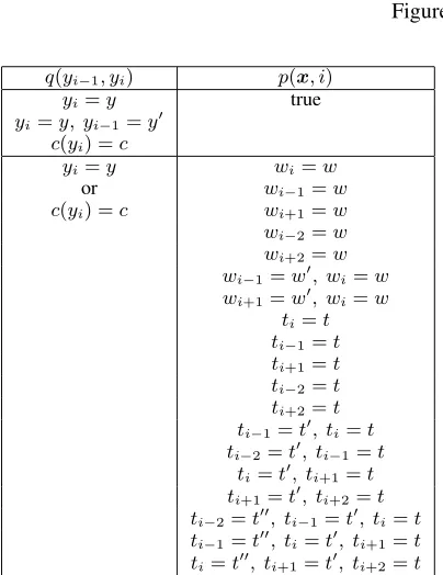
Our choice of features was mainly governed by com-puting power, since we do not use feature selection and all features are used in training and testing. We use the following factored representation for features
f(yi−1, yi,x, i) =p(x, i)q(yi−1, yi) (4)
wherep(x, i)is a predicate on the input sequencexand
current positioniandq(yi−1, yi)is a predicate on pairs
Rockwell International Corp. ’s Tulsa unit said it signed a tentative agreement extending its contract with Boeing Co. to provide structural parts for Boeing ’s 747 jetliners .
Figure 1: NP chunks
q(yi−1, yi) p(x, i)
yi=y true
yi=y, yi−1=y0 c(yi) =c
yi=y wi=w
or wi−1=w
c(yi) =c wi+1=w wi−2=w wi+2=w wi−1 =w0, wi=w wi+1=w0, wi=w
ti=t ti−1=t ti+1=t ti−2=t ti+2=t ti−1=t0, ti=t ti−2=t0, ti−1=t
ti=t0, ti+1=t ti+1=t0, ti+2=t ti−2=t00, ti−1=t0, ti=t ti−1=t00, ti=t0, ti+1=t ti=t00, ti
+1=t0, ti+2=t
Table 1: Shallow parsing features
DT,NN.” Because the label set is finite, such a factoring off(yi−1, yi,x, i)is always possible, and it allows each
input predicate to be evaluated just once for many fea-tures that use it, making it possible to work with millions of features on large training sets.
Table 1 summarizes the feature set. For a given po-sitioni,wi is the word,ti its POS tag, andyi its label.
For any label y = c0c, c(y) = c is the corresponding chunk tag. For example,c(OB) = B. The use of chunk tags as well as labels provides a form of backoff from the very small feature counts that may arise in a second-order model, while allowing significant associations be-tween tag pairs and input predicates to be modeled. To save time in some of our experiments, we used only the 820,000 features that aresupportedin the CoNLL train-ing set, that is, the features that are on at least once. For our highest F score, we used the complete feature set, around 3.8 million in the CoNLL training set, which con-tains all the features whose predicate is on at least once in the training set. The complete feature set may in princi-ple perform better because it can place negative weights on transitions that should be discouraged if a given pred-icate is on.
4.3 Parameter Tuning
As discussed previously, we need a Gaussian weight prior to reduce overfitting. We also need to choose the num-ber of training iterations since we found that the best F score is attained while the log-likelihood is still improv-ing. The reasons for this are not clear, but the Gaussian prior may not be enough to keep the optimization from making weight adjustments that slighly improve training log-likelihood but cause large F score fluctuations. We used the development test set mentioned in Section 4.1 to set the prior and the number of iterations.
4.4 Evaluation Metric
The standard evaluation metrics for a chunker are preci-sionP (fraction of output chunks that exactly match the reference chunks), recallR(fraction of reference chunks returned by the chunker), and their harmonic mean, the F1 scoreF1 = 2∗P ∗R/(P+R)(which we call just F score in what follows). The relationships between F score and labeling error or log-likelihood are not direct, so we report both F score and the other metrics for the models we tested. For comparisons with other reported results we use F score.
4.5 Significance Tests
Ideally, comparisons among chunkers would control for feature sets, data preparation, training and test proce-dures, and parameter tuning, and estimate the statistical significance of performance differences. Unfortunately, reported results sometimes leave out details needed for accurate comparisons. We report F scores for comparison with previous work, but we also give statistical signifi-cance estimates using McNemar’s test for those methods that we evaluated directly.
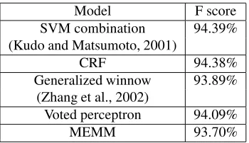
Model F score SVM combination 94.39% (Kudo and Matsumoto, 2001)
CRF 94.38%
Generalized winnow 93.89% (Zhang et al., 2002)
Voted perceptron 94.09%
[image:6.612.99.274.70.171.2]MEMM 93.70%
Table 2: NP chunking F scores
5 Results
All the experiments were performed with our Java imple-mentation of CRFs,designed to handle millions of fea-tures, on 1.7 GHz Pentium IV processors with Linux and IBM Java 1.3.0. Minor variants support voted perceptron (Collins, 2002) and MEMMs (McCallum et al., 2000) with the same efficient feature encoding. GIS, CG, and L-BFGS were used to train CRFs and MEMMs.
[image:6.612.334.520.70.147.2]5.1 F Scores
Table 2 gives representative NP chunking F scores for previous work and for our best model, with the com-plete set of 3.8 million features. The last row of the table gives the score for an MEMM trained with the mixed CG method using an approximate preconditioner. The pub-lished F score for voted perceptron is 93.53% with a dif-ferent feature set (Collins, 2002). The improved result given here is for the supported feature set; the complete feature set gives a slightly lower score of 94.07%. Zhang et al. (2002) reported a higher F score (94.38%) with gen-eralized winnow using additional linguistic features that were not available to us.
5.2 Convergence Speed
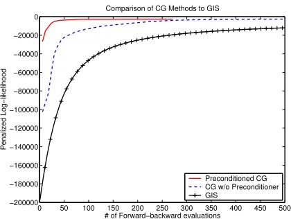
All the results in the rest of this section are for the smaller supported set of 820,000 features. Figures 2a and 2b show how preconditioning helps training convergence. Since each CG iteration involves a line search that may require several forward-backward procedures (typically between 4 and 5 in our experiments), we plot the progress of penalized log-likelihoodL0λ with respect to the num-ber of forward-backward evaluations. The objective func-tion increases rapidly, achieving close proximity to the maximum in a few iterations (typically 10). In contrast, GIS training increasesL0
λ rather slowly, never reaching the value achieved by CG. The relative slowness of it-erative scaling is also documented in a recent evaluation of training methods for maximum-entropy classification (Malouf, 2002). In theory, GIS would eventually con-verge to the L0
λ optimum, but in practice convergence may be so slow that L0
λ improvements may fall below numerical accuracy, falsely indicating convergence.
training method time F score L0 λ Precond. CG 130 94.19% -2968
Mixed CG 540 94.20% -2990 Plain CG 648 94.04% -2967 L-BFGS 84 94.19% -2948 GIS 3700 93.55% -5668
Table 3: Runtime for various training methods
null hypothesis p-value CRF vs. SVM 0.469 CRF vs. MEMM 0.00109 CRF vs. voted perceptron 0.116 MEMM vs. voted perceptron 0.0734
Table 4: McNemar’s tests on labeling disagreements
Mixed CG training converges slightly more slowly than preconditioned CG. On the other hand, CG without preconditioner converges much more slowly than both preconditioned CG and mixed CG training. However, it is still much faster than GIS. We believe that the superior convergence rate of preconditioned CG is due to the use of approximate second-order information. This is con-firmed by the performance of L-BFGS, which also uses approximate second-order information.2
Although there is no direct relationship between F scores and log-likelihood, in these experiments F score tends to follow log-likelihood. Indeed, Figure 3 shows that preconditioned CG training improves test F scores much more rapidly than GIS training.
Table 3 compares run times (in minutes) for reaching a target penalized log-likelihood for various training meth-ods with priorσ = 1.0. GIS is the only method that failed to reach the target, after 3,700 iterations. We cannot place the voted perceptron in this table, as it does not opti-mize log-likelihood and does not use a prior. However, it reaches a fairly good F-score above93%in just two training sweeps, but after that it improves more slowly, to a somewhat lower score, than preconditioned CG train-ing.
5.3 Labeling Accuracy
The accuracy rate for individual labeling decisions is over-optimistic as an accuracy measure for shallow pars-ing. For instance, if the chunkBIIIIIIIis labled as
OIIIIIII, the labeling accuracy is 87.5%, but recall is 0. However, individual labeling errors provide a more convenient basis for statistical significance tests. One
[image:6.612.334.515.183.248.2]6 56 106 156 206 256 −35000
−30000 −25000 −20000 −15000 −10000 −5000 0
# of Forward−backward evaluations
Penalized Log−likelihood
Comparison of Fast Training Algorithms for CRF
Preconditioned CG Mixed CG Training L−BFGS
(a)L0λ: CG (precond., mixed), L-BFGS
0 50 100 150 200 250 300 350 400 450 500 −200000
−180000 −160000 −140000 −120000 −100000 −80000 −60000 −40000 −20000 0
# of Forward−backward evaluations
Penalized Log−likelihood
Comparison of CG Methods to GIS
Preconditioned CG CG w/o Preconditioner GIS
[image:7.612.325.535.71.229.2](b)L0λ: CG (precond., plain), GIS
Figure 2: Training convergence for various methods
0 50 100 150 200 250 300 350 400 450 500
0.45 0.5 0.55 0.6 0.65 0.7 0.75 0.8 0.85 0.9 0.95
# of Forward−backward evaluations
F score
Comparison of CG Methods to GIS
[image:7.612.86.287.309.472.2]Preconditioned CG CG w/o Preconditioner GIS
Figure 3: Test F scoresvs.training time
such test is McNemar test on paired observations (Gillick and Cox, 1989).
With McNemar’s test, we compare the correctness of the labeling decisions of two models. The null hypothesis is that the disagreements (correctvs.incorrect) are due to chance. Table 4 summarizes the results of tests between the models for which we had labeling decisions. These tests suggest that MEMMs are significantly less accurate, but that there are no significant differences in accuracy among the other models.
6 Conclusions
We have shown that (log-)linear sequence labeling mod-els trained discriminatively with general-purpose opti-mization methods are a simple, competitive solution to learning shallow parsers. These models combine the best
features of generative finite-state models and discrimina-tive (log-)linear classifiers, and do NP chunking as well as or better than “ad hoc” classifier combinations, which were the most accurate approach until now. In a longer version of this work we will also describe shallow pars-ing results for other phrase types. There is no reason why the same techniques cannot be used equally successfully for the other types or for other related tasks, such as POS tagging or named-entity recognition.
On the machine-learning side, it would be interest-ing to generalize the ideas of large-margin classification to sequence models, strengthening the results of Collins (2002) and leading to new optimal training algorithms with stronger guarantees against overfitting.
On the application side, (log-)linear parsing models have the potential to supplant the currently dominant lexicalized PCFG models for parsing by allowing much richer feature sets and simpler smoothing, while avoid-ing the label bias problem that may have hindered earlier classifier-based parsers (Ratnaparkhi, 1997). However, work in that direction has so far addressed only parse reranking (Collins and Duffy, 2002; Riezler et al., 2002). Full discriminative parser training faces significant algo-rithmic challenges in the relationship between parsing al-ternatives and feature values (Geman and Johnson, 2002) and in computing feature expectations.
Acknowledgments
per-cepton results and compare his method with ours. Erik Tjong Kim Sang, who has created the best online re-sources on shallow parsing, helped us with details of the CoNLL-2000 shared task. Taku Kudo provided the out-put of his SVM chunker for the significance test.
References
S. Abney. Parsing by chunks. In R. Berwick, S. Abney, and C. Tenny, editors, Principle-based Parsing. Kluwer Aca-demic Publishers, 1991.
S. Abney, R. E. Schapire, and Y. Singer. Boosting applied to tagging and PP attachment. InProc. EMNLP-VLC, New Brunswick, New Jersey, 1999. ACL.
A. L. Berger, S. A. Della Pietra, and V. J. Della Pietra. A maxi-mum entropy approach to natural language processing.
Com-putational Linguistics, 22(1), 1996.
D. M. Bikel, R. L. Schwartz, and R. M. Weischedel. An algo-rithm that learns what’s in a name. Machine Learning, 34: 211–231, 1999.
L. Bottou. Une Approche th´eorique de l’Apprentissage
Con-nexionniste: Applications `a la Reconnaissance de la Parole.
PhD thesis, Universit´e de Paris XI, 1991.
E. Brill. Transformation-based error-driven learning and natural language processing: a case study in part of speech tagging.
Computational Linguistics, 21:543–565, 1995.
S. F. Chen and R. Rosenfeld. A Gaussian prior for smoothing maximum entropy models. Technical Report CMU-CS-99-108, Carnegie Mellon University, 1999.
M. Collins. Discriminative training methods for hidden Markov models: Theory and experiments with perceptron algo-rithms. InProc. EMNLP 2002. ACL, 2002.
M. Collins and N. Duffy. New ranking algorithms for parsing and tagging: Kernels over discrete structures, and the voted perceptron. InProc. 40th ACL, 2002.
J. N. Darroch and D. Ratcliff. Generalized iterative scaling for log-linear models.The Annals of Mathematical Statistics, 43 (5):1470–1480, 1972.
S. Della Pietra, V. Della Pietra, and J. Lafferty. Inducing fea-tures of random fields.IEEE PAMI, 19(4):380–393, 1997. B. Efron and R. J. Tibshirani.An Introduction to the Bootstrap.
Chapman & Hall/CRC, 1993.
D. Freitag and A. McCallum. Information extraction with HMM structures learned by stochastic optimization. In
Proc. AAAI 2000, 2000.
S. Geman and M. Johnson. Dynamic programming for parsing and estimation of stochastic unification-based grammars. In
Proc. 40th ACL, 2002.
L. Gillick and S. Cox. Some statistical issues in the compairson of speech recognition algorithms. InInternational
Confer-ence on Acoustics Speech and Signal Processing, volume 1,
pages 532–535, 1989.
J. Hammersley and P. Clifford. Markov fields on finite graphs and lattices. Unpublished manuscript, 1971.
T. Kudo and Y. Matsumoto. Chunking with support vector ma-chines. InProc. NAACL 2001. ACL, 2001.
J. Kupiec. Robust part-of-speech tagging using a hidden Markov model.Computer Speech and Language, 6:225–242, 1992.
J. Lafferty, A. McCallum, and F. Pereira. Conditional random fields: Probabilistic models for segmenting and labeling se-quence data. InProc. ICML-01, pages 282–289, 2001. R. Malouf. A comparison of algorithms for maximum entropy
parameter estimation. InProc. CoNLL-2002, 2002. A. McCallum, D. Freitag, and F. Pereira. Maximum entropy
Markov models for information extraction and segmentation.
InProc. ICML 2000, pages 591–598, Stanford, California,
2000.
T. P. Minka. Algorithms for maximum-likelihood logistic re-gression. Technical Report 758, CMU Statistics Department, 2001.
J. Nocedal and S. J. Wright.Numerical Optimization. Springer, 1999.
V. Punyakanok and D. Roth. The use of classifiers in sequential inference. InNIPS 13, pages 995–1001. MIT Press, 2001.
L. A. Ramshaw and M. P. Marcus. Text chunking using
transformation-based learning. InProc. Third Workshop on
Very Large Corpora. ACL, 1995.
A. Ratnaparkhi. A maximum entropy model for part-of-speech tagging. InProc. EMNLP, New Brunswick, New Jersey, 1996. ACL.
A. Ratnaparkhi. A linear observed time statistical parser based on maximum entropy models. In C. Cardie and R. Weischedel, editors,EMNLP-2. ACL, 1997.
S. Riezler, T. H. King, R. M. Kaplan, R. Crouch, J. T. Maxwell III, and M. Johnson. Parsing the Wall Street Journal using a lexical-functional grammar and discriminative esti-mation techniques. InProc. 40th ACL, 2002.
E. F. T. K. Sang. Memory-based shallow parsing. Journal of
Machine Learning Research, 2:559–594, 2002.
J. R. Shewchuk. An introduction to the conjugate gradient method without the agonizing pain, 1994. URLhttp:// www-2.cs.cmu.edu/˜jrs/jrspapers.html#cg. B. Taskar, P. Abbeel, and D. Koller. Discriminative
probabilis-tic models for relational data. InEighteenth Conference on
Uncertainty in Artificial Intelligence, 2002.
E. F. Tjong Kim Sang and S. Buchholz. Introduction to the CoNLL-2000 shared task: Chunking. InProc. CoNLL-2000, pages 127–132, 2000.
H. Wallach. Efficient training of conditional random fields. In
Proc. 6th Annual CLUK Research Colloquium, 2002.
A. Yeh. More accurate tests for the statistical significance of result differences. InCOLING-2000, pages 947–953, Saar-bruecken, Germany, 2000.
T. Zhang, F. Damerau, and D. Johnson. Text chunking based on a generalization of winnow.Journal of Machine Learning