Using Reinforcement Learning to Model Incrementality in a Fast Paced Dialogue Game

Using Reinforcement Learning to Model Incrementality

in a Fast-Paced Dialogue Game

Ramesh Manuvinakurike1,2_{, David DeVault}2_{, Kallirroi Georgila}1,2 1_{Institute for Creative Technologies, University of Southern California}

2_{Computer Science Department, University of Southern California} manuvina|[email protected], [email protected]

Abstract

We apply Reinforcement Learning (RL) to the problem of incremental dialogue pol-icy learning in the context of a fast-paced dialogue game. We compare the policy learned by RL with a high performance baseline policy which has been shown to perform very efficiently (nearly as well as humans) in this dialogue game. The RL policy outperforms the baseline policy in offline simulations (based on real user data). We provide a detailed comparison of the RL policy and the baseline policy, includ-ing information about how much effort and time it took to develop each one of them. We also highlight the cases where the RL policy performs better, and show that un-derstanding the RL policy can provide valu-able insights which can inform the creation of an even better rule-based policy.

1 Introduction

Building incremental spoken dialogue systems (SDSs) has recently attracted much attention. One reason for this is that incremental dialogue pro-cessing allows for increased responsiveness, which in turn improves task efficiency and user satisfac-tion. Incrementality in dialogue has been studied in the context of turn-taking, predicting the next user utterances/actions, and generating fast system

re-sponses (Skantze and Schlangen,2009;Schlangen

et al.,2009;Selfridge and Heeman,2010;DeVault et al., 2011; Dethlefs et al., 2012a,b; Selfridge et al.,2012,2013;Hastie et al.,2013;Baumann and Schlangen,2013;Paetzel et al., 2015). Over the years researchers have tried a variety of approaches to incremental dialogue processing. One such ap-proach is using rules whose parameters may be

optimized using real user data (Buß et al., 2010;

Ghigi et al.,2014;Paetzel et al.,2015). Reinforce-ment Learning (RL) is another method that has been used to learn policies regarding when the sys-tem should interrupt the user (barge-in), stay silent, or generate backchannels in order to improve the responsiveness of the SDS or increase task success (Kim et al.,2014;Khouzaimi et al.,2015;Dethlefs et al.,2016).

We apply RL to the problem of incremental dia-logue policy learning in the context of a fast-paced dialogue game. We use a corpus of real user data for both training and testing. We compare the poli-cies learned by RL with a high performance base-line policy which uses parameterized rules (whose parameters have been optimized using real user data) and has a carefully designed rule (CDR) struc-ture. From now on, we will refer to this baseline as the CDR baseline.

Our contributions are as follows: We provide an RL method for incremental dialogue processing based on simplistic features which performs better in offline simulations (based on real user data) than the high performance CDR baseline. Note that this is a very strong baseline which has been shown to perform very efficiently (nearly as well as

hu-mans) in this dialogue game (Paetzel et al.,2015).

In many studies that use RL for dialogue policy learning, the focus is on the RL algorithms, the state-action space representation, and the reward function. As a result, the rule-based baselines used for comparing the RL policies against are not as carefully engineered as they could be, i.e., they are not the result of iterative improvement and opti-mization using insights learned from data or user testing. This is understandable since building a very strong baseline would be a big project by itself and would detract attention from the RL problem. In our case, there was a pre-existing strong CDR base-line policy which inspired us to investigate whether it could be outperformed by an RL policy. One of

our main contributions is that we provide a detailed comparison of the RL policy and the CDR baseline policy, including information about how much ef-fort and time it took to develop each one of them. We also highlight the cases where the RL policy performs better, and show that understanding the RL policy can provide valuable insights which can inform the creation of an even better rule-based policy.

2 RDG-Image Game

For this study we used the RDG-Image (Rapid

Di-alogue Game) (Paetzel et al., 2014) dataset and

the high performance baseline Eve system

(Sec-tion 2.2). RDG-Image is a collaborative, two

player, time-constrained, incentivized rapid con-versational game, and has two player roles, the Director and the Matcher. The players are given 8

images as shown in Figure1in a randomized order.

One of the images is highlighted with a red border on the Director’s screen (called target image - TI). The Matcher sees the same 8 images in a different order but does not know the TI. The Director has to describe the TI in such a way that the Matcher will be able to identify it from the distractors as quickly as possible. The Director and Matcher can talk back-and-forth freely to accomplish the task. Once the Matcher believes that he has made the right se-lection, he clicks on the image and communicates this to the Director. If the guess is correct then the team earns 1 point, otherwise 0 points. Now the Director can press a button so that the game can continue with a new TI. The game consists of 4 rounds called Sets (from 1 - 4) with varying levels of complexity. Each round has a predefined time limit. The goal is to complete as many images as possible, and thus as a team to earn as many points as possible.

2.1 Human-Human Data

The RDG-Image data comes in two flavors, human-human (HH) and human-human-agent (HA) spoken con-versations. The HH data was collected by pairing 2 human players in real time and having their con-versation recorded. The HA concon-versations were recorded by pairing a human Director with the

agent Matcher (Section2.2). In this section, we

de-scribe the HH part of the corpus. The HH data was

collected in two separate experiments, in-lab (

Paet-zel et al.,2014) and over the web (Manuvinakurike and DeVault, 2015). Figure1 shows an excerpt

from the HH corpus.

The HH corpus contains the user speech tran-scribed, and labeled dialogue acts (DAs) along with carefully annotated time stamps as shown in

Figure 1. This timing information is important

for modeling incrementality. We can observe that the game conversation involves rapid exchanges with frequent overlaps. Each episode (dialogue exchange for each TI) typically begins with the Di-rector describing the TI and ends with the Matcher acknowledging the TI selection with the Assert-Identified (As-I) DA (e.g., “got it”) or As-S (skip-ping action) DA (e.g., “let’s move on to the next image”). The Director then requests the next TI and the game continues until time runs out. Some-times the Matcher may interrupt the Director with questions or other illocutionary acts. A complete

list of DAs can be found in (Manuvinakurike et al.,

2016).

In this paper, we are interested in modeling in-crementality for DAs related to TI selection by the Matcher. As-I is the most common DA used by the human Matchers. As-S was not frequently used by the human Matchers but is used by the base-line matcher agent to give up on the current TI and proceed to the next TI to try to increase the total points scored. Further distinctions between

As-I and As-S are made in Section2.2. The most

common DA generated by the Director was D-T (Describe-Target).

2.2 Eve

The baseline agent called Eve (Paetzel et al.,2015)

was developed to play the role of the Matcher using the HH data. The agent Eve relies on several kinds of incremental processing. It obtains the 1-best automatic speech recognition (ASR) hypothesis every 100ms and forwards it to the natural language understanding (NLU) module. The NLU module is a Naive Bayes classifier trained on bag-of-words features which are generated using a frequency threshold (frequency >5) on unigrams and bigrams

(dt). The NLU assigns confidence values to the

8 images (called the image set). Let the image

set at timetbeIt ={i1, ..., i8}, with the correct

target imageT ∈ Itunknown to the agent. The

maximum probability assigned to any image at time

t is P∗

t = maxjP(T = ij|dt). We call these

probability values (P(T = ij|dt)) as confidence.

The image with the highest confidence is chosen

Figure 1: Example interaction for a set of images in the human-human corpus.

time consumed on the current TI.

Eve’s policy decides between waiting and inter-rupting the user with As-I or As-S to maximize the score in the game. She can do it by taking three actions: i) WAIT: Listen more in the hope that the user provides more information; ii) As-I: Make the selection and request the next TI; iii) As-S: Make the selection and request the next TI as it might

not be fruitful to wait more.1 _{Eve’s policy depicted}

in Algorithm1, uses two threshold values namely

identification threshold (IT) and give-up threshold (GT) to select these actions. The IT learned is

the least confidence value (P∗

t) above which the

agent uses the As-I action. GT is the maximum time the agent should WAIT before giving up on the current image set and requesting the human Director to move on to the next TI. The IT and GT values are learned using an offline policy optimiza-tion method called the Eavesdropper simulaoptimiza-tion, which performs an exhaustive grid search to find the optimal values of IT and GT for each image

set (Paetzel et al., 2015). In this simulation, the

agent is trained offline on the HH conversations and learns the best values of IT and GT, i.e., the values that result in scoring the maximum points in the game. For example, the optimal values learned

for the image set shown in Figure1were IT=0.8

and GT=18sec.

The Eve agent is very efficient and carefully en-gineered to perform well in this task, and serves as a very strong baseline. In the real user study

reported in Paetzel et al.(2015), Eve in the HA

gameplay scored nearly as well as human users in HH gameplay. Thus this study provides an opportu-nity to compare an RL policy with a strong baseline

1_{For As-S Eve’s utterance is ‘I don’t think I can get that}

one. Let’s move on. I clicked randomly’ and for As-I it is ‘Got it’.

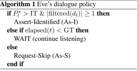
Algorithm 1Eve’s dialogue policy

ifP∗

t >IT &|filtered(dt)| ≥1then

Assert-Identified (As-I)

else ifelapsed(t)<GTthen

WAIT (continue listening)

else

Request-Skip (As-S)

end if

policy that uses a hand-crafted carefully designed rule structure (CDR baseline). In the Appendix,

Figure6 shows an example from the HA corpus.

The data used in the current work comes from both

the HH and HA datasets (see Table1).

Branch # users # sub-dialogues

Human-Human lab 64 1485

Human-Human web 196 5642

Human-Agent web 175 7393

Table 1: Number of users and number of TI sub-dialogues used for our study.

2.3 Improving NLU with Agent Conversation Data

Obviously, the success of the agent heavily depends on the accuracy of the NLU module. In the earlier

work by Paetzel et al. (2015), the NLU module

across all sets of images2_{. Thus in this work we}

use the best performing NLU with the data trained from both the HH and HA subsets of the corpus. The overall reported NLU accuracy was averaged across all the image sets. The NLU module was

trained with the same method as inPaetzel et al.

(2015). Note that for all our experiments, 10% of

the HH data and 10% of the HA data was used for testing, and the rest was used for training.

2.4 Room for Improvement

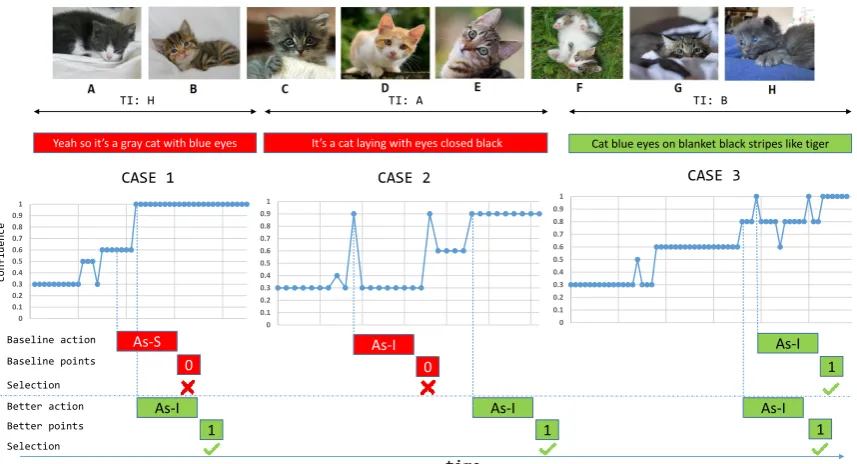
Though the baseline agent is impressive in its per-formance there are a few shortcomings. We in-vestigated the errors being made by the baseline policy and identified four primary limitations in its decision-making. Examples of these limitations

are shown in Figure2, depicting the NLU assigned

confidence (y-axis) for the human TI descriptions plotted against the time steps (x-axis).

First, the baseline commits to As-I as soon as the confidence reaches a high enough value (IT thresh-old), or As-S when the time consumed exceeds the GT threshold. In Case 1 the agent decides to skip (As-S) because the time consumed has exceeded the GT threshold, instead of waiting more which would allow for a more distinguishing description to come from the human Director.

Second, its performance can be negatively af-fected by instability in the partial ASR results.

Ex-amples of partial ASR results are shown in Figure8

in the Appendix. In Case 2, the agent could learn to wait for higher time intervals as the ASR partial outputs become more stable.

Third, the baseline only commits at high confi-dence values. Case 3 shows an instance where the agent can save time by committing to a selection at a much lesser confidence value.

Fourth, as we can see from Algorithm1, the

base-line policy does not use “combinations” (or joint values) of time and confidence to make detailed decisions.

Perhaps using RL can not only help the agent learn a more complex strategy but could also pro-vide insights into developing a better engineered policy which would not have been intuitive for a di-alogue designer to come up with. That is, RL could potentially help in building better rules that would be much easier to incorporate into the agent and thus improve its performance. For example, is there

2_{All the significance tests are performed using student’s t}

test.

a combination of time and confidence which is not currently used by the baseline i.e., not committing at some initial time slices for high confidence val-ues and committing at lower confidence valval-ues as the user consumes more time?

3 Design of the RL Policy

The incremental policy decision making is mod-eled as an MDP (Markov decision process), i.e.,

a tuple(S, A, T P, R, γ). S is a set of states that

the agent can be in. In this taskSis represented

by(P∗

t, tc)features wherePt∗ is the highest

con-fidence score assigned by the NLU for any image

in the image set (P∗

t 7−→ IR; 0.0 ≤ Pt∗ ≤ 1.0)

and tc is the time consumed for the current TI

(tc 7−→ IR; 0.0 ≤ tc ≤ 45.0)3. The RL learns

a policyπmapping the state (S) to the action (A),

π:S →A, whereA= {As-I, As-S, WAIT} are the

actions to be performed by the agent to maximize the overall reward in the game. The As-I and As-S

actions map to their corresponding utterances.Ris

the reward function andγa discount factor

weight-ing long-term rewards. TP is the set of transition probabilities after taking an action.

When the agent is in the state St = (Pt∗, tc),

executing the WAIT action results in moving to

the state St+1 which corresponds to a new dt+1

which corresponds to the new utterance (See

Sec-tion2.2) and thus yielding newP∗

t andtcfor the

given episode. The As-I and As-S actions result in goal states for the agent. Separate policies are trained per image set similar to the baseline. The difference between the As-I and As-S action is in

the rewards assigned. The reward functionRis as

follows. After the agent performs the As-I action, it receives a high positive reward for the correct image selection and a high negative penalty for the wrong selection. This is to encourage the agent to learn to guess at the right point of time. There is

a small positive reward ofδfor “WAIT” actions,

to encourage the agent to wait before committing to As-I selections. No reward is provided for the As-S actions. This is to discourage the agent from choosing to skip and scoring the points by chance, and at the same time not penalize the agent for wanting to skip when it is really necessary. The reward function for As-S prevents the agent from getting heavy negative penalties in case the wrong images are selected by the NLU. In those cases the confidence would probably be low and thus the

TI: H TI: A TI: B

Yeah so it’s a gray cat with blue eyes It’s a cat laying with eyes closed black Cat blue eyes on blanket black stripes like tiger

0 0.1 0.2 0.3 0.4 0.5 0.6 0.7 0.8 0.9 1 0 0.1 0.2 0.3 0.4 0.5 0.6 0.7 0.8 0.9 1 0 0.1 0.2 0.3 0.4 0.5 0.6 0.7 0.8 0.9 1 As-I As-I As-I As-I As-I Baseline action Better action time confide nce

CASE 1 CASE 2 CASE 3

Baseline points

Better points

0 0 1

1 1 1

Selection Selection

As-S

Figure 2: Examples where the agent can do better. The red boxes show the wrong selection by the agent.

agent would not commit to As-I but choose the action As-S instead.

R=         

+δ if action is WAIT +100 if As-I is right −100 if As-I is wrong 0 if action is As-S

In this work we use the least squares policy

it-eration (LSPI) (Lagoudakis and Parr, 2003) RL

algorithm implemented in the BURLAP4_{java code}

library to learn the optimal policy. LSPI is a sample efficient model-free off-policy method that com-bines policy iteration with linear value function ap-proximation. LSPI in our work uses State-Action-Reward-State (SARS) transitions sampled from the human interactions data (HH and HA). We use Gaussian radial basis value function (RBF)

rep-resentation for the confidence (P∗

t) and time

con-sumed (tc) features. We treat the state features

as continuous values. The confidence values and time consumed values are continuous in nature

within the bounds defined i.e., 0.0 ≤ P∗

t ≤ 1.0

and0.0≤tc≤45.0. We define 10 basis functions

distributed uniformly for the confidence features

(P∗

t) and 45 basis functions for the time consumed

(tc) features. The basis function returns a value

between 0 and 1 with a value of 1 when the query state has a distance of zero from the function’s “center” state. As the state gets further away, the

4_{http://burlap.cs.brown.edu/}

basis function’s returned value degrades to a value of zero.

Initial experimentation with the Vanilla

Q-learning algorithm (Sutton and Barto, 1998) did

not yield good results, due to the very large state space and consequently data sparsity. Binning the features, in order to transform their continuous val-ues into discrete valval-ues and thus reduce the size of the state space, did not help either. That is, hav-ing a large number of bins did not deal with the data sparsity problem, and having a small number of bins made it much harder to learn fine-grained distinctions between the states. Note that LSPI is generally considered as a more sample efficient algorithm than Q-learning.

We run LSPI with a discount factor of 0.99 until convergence occurs or a maximum of 50 iterations is reached, whichever happens first. We use 250k available SARS transitions from the HH and HA interactions to train the policy. The LSPI returns a Greedy-Q policy which we use on the test data.

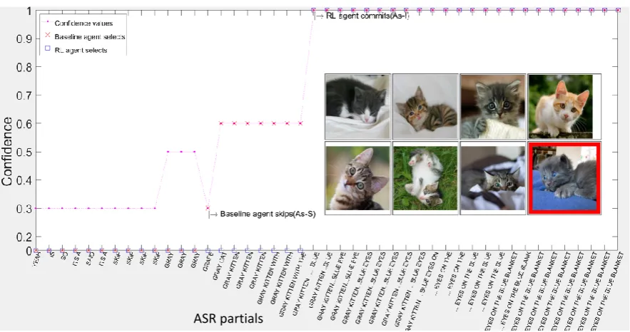
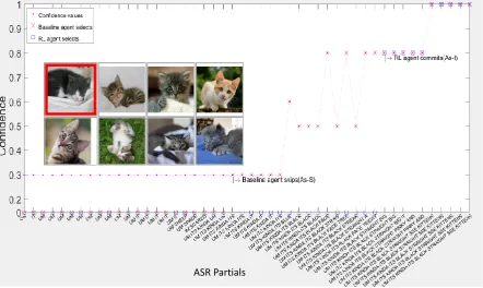
Figure3shows the modus operandi of the

pol-icy in this domain. For every time step the ASR provides a 1-best partial hypothesis for the speech uttered by the test user. This partial speech recogni-tion hypothesis is input to the NLU module which

returns the confidence value (P∗

t). The time

con-sumed (tc) for the current TI is tracked by the game

ASR partials

Figure 3: Actions taken by the baseline and the RL agent.

pets zoo kitten cocktail bikes yoga necklace

PPS P PPS P PPS P PPS P PPS P PPS P PPS P

Baseline 0.22 37 0.28 27 0.14 14 0.18 23 0.09 13 0.20 3 0.20 4

RL agent 0.23 39 0.31 32 0.13 16 0.19 25 0.14 22 0.11 18 0.12 20

Table 2: Comparison of points per second (PPS) and points (P) earned by the baseline and the RL agent on the test set.

4 Experimental Setup

For testing, we use the real user held out conver-sation data from the HH and HA datasets. The IT and GT thresholds for the baseline Eve were

also retrained (Paetzel et al.,2015) using the same

data and NLU as used to train the RL policy.

Fig-ure3shows the setup for testing and comparing the

actions of the RL policy and the baseline. Every ASR partial corresponds to a state. For every ASR partial we obtain the highest assigned confidence score from the NLU, use the time consumed fea-ture from the game, and obtain the action from the policy. If the action chosen by the policy is “WAIT” then we sample the next state. For each pair of confidence and time consumed values we obtain the actions from the baseline and the RL policy separately and compare them with the ground truth to evaluate which policy performs better. Once the policy decides to take either the As-I or As-S action then we advance the simulated game time by an ad-ditional interval of 750ms or 1500ms respectively. This is to simulate the conditions in the real user game where we found that the users on average

take 500ms to click the button to load the next set of TIs, and the agent takes 250ms to say the As-I utterance and 1000ms to say the As-S utterance. The next TI is loaded at this point and then the process is repeated until the game time runs out for each user round.

5 Results

The policy learned using RL (LSPI with RBF func-tions) performs significantly better (p<0.01) in scor-ing points compared to the baseline agent in offline simulations. Also, the RL policy takes relatively more time to commit (As-I or As-S) compared to

the baseline.5 _{The idea of setting the IT and GT}

threshold values in the baseline (Section2.2)

origi-nally aimed at scoring points rapidly in the game, i.e., the baseline agent was optimized at scoring the highest number of points per second (PPS). The PPS parameter is a measure of how effective the agent is at scoring points overall, and is calcu-lated as the ratio of the total points scored by the

5_{p=0.06; we cannot claim that the time taken is}

0 20 40 60 80 100 120 140 160

0 2 4 6 8 10 12 14 16 18 20 22 Baseline RL(LSPI)

Average Points scored

Time c

ons

umed

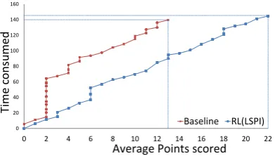
Figure 4: The RL policy scores significantly more points than the baseline by investing slightly more time (graph generated for one of the image sets).

agent divided by the total time consumed. Table2

shows the points per second and the total points scored in some of the image sets by the baseline and the RL. We can observe that the RL consistently scores more points than the baseline, however this comes at the cost of additional time. By scoring more points overall than the baseline, the RL also

scores higher in the PPS metric (p<0.05). Table3

shows the total points scored and the total time spent across all the users by the baseline and the agent. Each set here refers to one round in a game.

Baseline RL

Set P t (s) P t (s) 1 96 510.8 107 528.1 2 75 525.0 85 537.9 3 42 298.9 74 595.2 4 49 531.9 76 592.3

Table 3: The points scored (P) and the time con-sumed (t) in seconds for different image sets (Set).

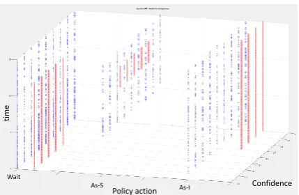
Figure 5: Decisions of the RL policy (in blue) vs. the baseline policy (in red).

Figure4depicts this result for an image set of

bikes (images shown in Figure 1). We plot the

total time spent by the agent and the total points

scored. Clearly, the RL policy manages to score more points than the baseline in a given amount of time. In order to understand the differences in the actions taken by the RL policy and the baseline policy, we plot on a 3 dimensional scatter plot, the action taken by the policy for confidence values between 0 and 1 (spaced at 0.1 intervals) and the time consumed between 0s to 15s (spaced at 100ms intervals) for one of the image sets (bikes).

Fig-ure5shows the decisions made by the RL (in blue)

compared to the decisions made by the baseline (in red). As we can see there is not much variety in the decisions of the baseline policy; it basically uses

thresholds (see Algorithm1) optimized using real

user data. Below we summarize our observations regarding the actions taken by the RL policy.

i) Regardless of whether the confidence value is high or low, the RL policy learns to wait for low val-ues of the time consumed. This may be helping the RL policy to avoid the problem illustrated in Case 2

in Figure2, where instability in the early ASR

re-sults for a description can lead an incorrect guess to be momentarily associated with high confidence. The RL policy is more keen on waiting and decides to commit early only when the confidence value is really high (almost 1.0). ii) Requiring a lower degree of confidence when the time consumed is high was also found to be an effective strategy to score more points in the game. Thus the RL policy learns to guess (As-I) even at lower confidence val-ues when the time consumed reaches high valval-ues. This combination of time and confidence values helps the RL agent perform better w.r.t. points and consequently PPS in the task.

It is also important to note that the agent does not wait eternally to make its selection. The human TI descriptions are collected from real user gameplay that lasts for a limited number of time steps. That is, the maximum number of points that the RL policy can score in simulation is limited by the number of images described in the real user gameplay. In the case of the “WAIT” action beyond this point the agent fails to gather high rewards as the As-I action was never selected. By the virtue of this design feature, the RL agent has implicitly learned the notion of playing the game at a high pace.

Note also that the RL agent has not learned to always commit at a later time than the baseline.

Table4shows the percentage of times (in the test

% times Same commit times 48.06 % times Baseline has faster commit 44.77 % times RL has faster commit 7.17

Table 4: Comparison of commit strategies between baseline and RL (%).

policy commits at the same time instances as the baseline about 48% of the time. 44.77% of the time the baseline commits to the TI faster and about 7% of the time the RL decides to commit earlier to the TI compared to the baseline.

6 Discussion & Future Work

The cases shown in Figure2provide examples of

how the RL policy can outperform the baseline. i) As the RL agent has learned to not commit to a decision early it can wait enough time to observe more user words and thus reach higher confidence (Case 1). ii) The RL agent is not keen on commit-ting when it sees an early high confidence value (like IT for the baseline) but rather waits which may enable the ASR partials to become more sta-ble (Case 2). iii) The RL agent also learns to com-mit at low confidence values as the time consumed increases and sometimes even committing earlier than the baseline (Case 3).

6.1 Contrasting Baseline and RL Policy Building Efforts

Building an SDS with carefullly crafted rules has often been criticized as a laborious and time con-suming exercise. This is in contrast to the alter-native data oriented approaches, which are often argued to require less time to engineer a solution and be more scalable. Development of the baseline system’s policy component took an NLP researcher approximately two months, including experimen-tation with alternative rule structures and devel-opment of the parameter optimization framework. Note that this effort does not include data collec-tion. The same amount of effort was put into devel-oping the RL policy by a researcher with similar skills. Building the RL policy involved experiment-ing with various reward functions to suit the task. Though the reward function is simplistic in our case, a high negative reward for wrong As-I actions was required for RL to learn useful policies. It also takes effort and experimentation to select the right algorithm (LSPI with value function approxima-tion vs. Vanilla Q-learning). It is thus hard to claim which approach is more time-efficient (in terms

of development effort). Figure7in the Appendix

shows a comparison of the baseline policy and the RL policy learned with the Vanilla Q-learning al-gorithm which did not perform well. It performed worse than the baseline. We also need to keep in mind that: i) We cannot claim that the rules learned by the RL policy could not be implemented in the hand-crafted system. Bounds on the time and con-fidence (for example: do not commit as soon as the confidence exceeds a threshold but rather wait for a few additional time steps, it is okay to commit at lower confidence values for higher time values to perform better, etc.) can be included in the

Al-gorithm1 and the system can be deployed with

ease. ii) It usually takes time and effort to build a common infrastructure to experiment between the two strategies. In this case, experimenting with the incremental RL policy was simpler as the in-frastructure and the methodology existed from the

previous work byManuvinakurike et al.(2015) and

Paetzel et al.(2015). Despite the fact that both ap-proaches required similar development effort, in the end, RL did learn a better strategy automati-cally, at least in our offline simulations (based on real user data). RL provides advantages compared to the baseline method. Adding new constraints into the baseline can be hard. This is because the baseline method uses exhaustive grid search to set its parameter values, and it might be exponentially costly to do this with more constraints. On the other hand, RL is more scalable as adding features is relatively easy with RL.

6.2 Future Work

the high performance CDR baseline and see which avenue would be more fruitful and if we can get the best of both worlds. Finally, another idea for future work is to experiment with Inverse Reinforcement

Learning (Abbeel and Ng,2004;Nouri et al.,2012;

Kim et al., 2014) in order to potentially learn a better reward function directly from the data.

Acknowledgments

This work was supported by the National Science Foundation under Grant No. IIS-1219253 and by the U.S. Army Research Laboratory (ARL) un-der contract number W911NF-14-D-0005. Any opinions, findings, and conclusions or recommen-dations expressed in this material are those of the author(s) and do not necessarily reflect the views, position, or policy of the National Science Foun-dation or the United States Government, and no official endorsement should be inferred. We would like to thank Maike Paetzel. Thanks to Hugger Industries, Eric Sorenson and fixedgear for images published under CC BY-NC-SA 2.0. Thanks to Eric Parker and cosmo flash for images published under CC BY-NC 2.0, and to Richard Masonder / Cyclelicious and Florian for images published under CC BY-SA 2.0. Thanks to wikimedia for images published under CC BY-SA 2.0.

References

Pieter Abbeel and Andrew Y. Ng. 2004. Apprentice-ship learning via inverse reinforcement learning. In Proceedings of the International Conference on Ma-chine Learning (ICML). Banff, Alberta, Canada. Timo Baumann and David Schlangen. 2013.

Open-ended, extensible system utterances are preferred,

even if they require filled pauses. InProceedings of

the Annual Meeting of the Special Interest Group on Discourse and Dialogue (SIGDIAL). Metz, France, pages 280–283.

Okko Buß, Timo Baumann, and David Schlangen. 2010. Collaborating on utterances with a spoken di-alogue system using an ISU-based approach to

incre-mental dialogue management. InProceedings of the

Annual Meeting of the Special Interest Group on Dis-course and Dialogue (SIGDIAL). pages 233–236. Nina Dethlefs, Helen Hastie, Heriberto Cuayáhuitl,

Yanchao Yu, Verena Rieser, and Oliver Lemon. 2016. Information density and overlap in spoken dialogue. Computer Speech & Language37:82–97.

Nina Dethlefs, Helen Hastie, Verena Rieser, and Oliver Lemon. 2012a. Optimising incremental dialogue de-cisions using information density for interactive

sys-tems. In Proceedings of the Joint Conference on

Empirical Methods in Natural Language Process-ing and Computational Natural Language LearnProcess-ing (EMNLP-CoNLL). Jeju Island, South Korea, pages 82–93.

Nina Dethlefs, Helen Hastie, Verena Rieser, and Oliver Lemon. 2012b. Optimising incremental generation for spoken dialogue systems: Reducing the need for

fillers. InProceedings of the International Natural

Language Generation Conference (INLG). Utica, IL, USA, pages 49–58.

David DeVault, Kenji Sagae, and David Traum. 2011. Incremental interpretation and prediction of

utter-ance meaning for interactive dialogue. Dialogue &

Discourse2(1).

Fabrizio Ghigi, Maxine Eskenazi, M. Ines Torres, and Sungjin Lee. 2014. Incremental dialog processing

in a task-oriented dialog. InProceedings of

INTER-SPEECH. Singapore, pages 308–312.

Helen Hastie, Marie-Aude Aufaure, Panos Alexopou-los, Heriberto Cuayáhuitl, Nina Dethlefs, Milica Gaši´c, James Henderson, Oliver Lemon, Xingkun Liu, Peter Mika, Nesrine Ben Mustapha, Verena Rieser, Blaise Thomson, Pirros Tsiakoulis, Yves Vanrompay, Boris Villazon-Terrazas, and Steve Young. 2013. Demonstration of the Parlance system: a data-driven, incremental, spoken dialogue system

for interactive search. InProceedings of the Annual

Meeting of the Special Interest Group on Discourse and Dialogue (SIGDIAL). Metz, France, pages 154– 156.

Hatim Khouzaimi, Romain Laroche, and Fabrice Lefèvre. 2015. Optimising turn-taking strategies

with reinforcement learning. InProceedings of the

Annual Meeting of the Special Interest Group on Dis-course and Dialogue (SIGDIAL). Prague, Czech Re-public, pages 315–324.

Dongho Kim, Catherine Breslin, Pirros Tsiakoulis, Mil-ica Gaši´c, Matthew Henderson, and Steve Young. 2014. Inverse reinforcement learning for micro-turn

management. In Proceedings of INTERSPEECH.

Singapore, pages 328–332.

Michail G. Lagoudakis and Ronald Parr. 2003.

Least-squares policy iteration. Journal of Machine

Learn-ing Research4:1107–1149.

Ramesh Manuvinakurike and David DeVault. 2015. Natural Language Dialog Systems and Intelligent Assistants, chapter Pair Me Up: A web framework for crowd-sourced spoken dialogue collection, pages 189–201.

Ramesh Manuvinakurike, Maike Paetzel, and David

DeVault. 2015. Reducing the cost of dialogue

system training and evaluation with online,

crowd-sourced dialogue data collection. InProceedings of

Ramesh Manuvinakurike, Maike Paetzel, Cheng Qu, David Schlangen, and David DeVault. 2016. Toward incremental dialogue act segmentation in fast-paced

interactive dialogue systems. InProceedings of the

Annual Meeting of the Special Interest Group on Dis-course and Dialogue (SIGDIAL). Los Angeles, CA, USA, pages 252–262.

Elnaz Nouri, Kallirroi Georgila, and David Traum. 2012. A cultural decision-making model for

negotia-tion based on inverse reinforcement learning. In

Pro-ceedings of the Annual Meeting of the Cognitive Sci-ence Society (CogSci). Sapporo, Japan, pages 2097– 2102.

Maike Paetzel, Ramesh Manuvinakurike, and David DeVault. 2015. “So, which one is it?” The effect of alternative incremental architectures in a

high-performance game-playing agent. InProceedings of

the Annual Meeting of the Special Interest Group on Discourse and Dialogue (SIGDIAL). Prague, Czech Republic, pages 77–86.

Maike Paetzel, David Nicolas Racca, and David De-Vault. 2014. A multimodal corpus of rapid dialogue

games. InProceedings of the Language Resources

and Evaluation Conference (LREC). Reykjavik, Ice-land, pages 4189–4195.

David Schlangen, Timo Baumann, and Michaela At-terer. 2009. Incremental reference resolution: The task, metrics for evaluation, and a Bayesian filtering

model that is sensitive to disfluencies. In

Proceed-ings of the Annual Meeting of the Special Interest Group on Discourse and Dialogue (SIGDIAL). Lon-don, UK, pages 30–37.

Ethan Selfridge, Iker Arizmendi, Peter Heeman, and Jason Williams. 2013. Continuously predicting and processing barge-in during a live spoken dialogue

task. InProceedings of the Annual Meeting of the

Special Interest Group on Discourse and Dialogue (SIGDIAL). Metz, France, pages 384–393.

Ethan Selfridge and Peter Heeman. 2010. Importance-driven turn-bidding for spoken dialogue systems. In Proceedings of the 48th Annual Meeting of the As-sociation for Computational Linguistics (ACL). Up-psala, Sweden, pages 177–185.

Ethan O. Selfridge, Iker Arizmendi, Peter A. Heeman, and Jason D. Williams. 2012. Integrating incremen-tal speech recognition and POMDP-based dialogue

systems. InProceedings of the Annual Meeting of

the Special Interest Group on Discourse and Dia-logue (SIGDIAL). Seoul, South Korea, pages 275– 279.

Gabriel Skantze and David Schlangen. 2009. Incre-mental dialogue processing in a micro-domain. In Proceedings of the 12th Conference of the European Association for Computational Linguistics (EACL). Athens, Greece, pages 745–753.

Richard S. Sutton and Andrew G. Barto. 1998.

Re-inforcement learning: An introduction. MIT Press Cambridge.

Appendix

Example dialogue

Figure 6: Example dialogue for an episode in the

human-agent corpus for the same TI as in Figure1.

Policy differences

Policy action Confidence

time

Wait

As-S _As-S

As-I

ASR Partials