Human Language Technologies: The 2009 Annual Conference of the North American Chapter of the ACL, pages 539–547,
Optimal Reduction of Rule Length
in Linear Context-Free Rewriting Systems
Carlos G´omez-Rodr´ıguez1, Marco Kuhlmann2, Giorgio Satta3and David Weir4
1Departamento de Computaci´on, Universidade da Coru˜na, Spain ([email protected])
2Department of Linguistics and Philology, Uppsala University, Sweden ([email protected])
3Department of Information Engineering, University of Padua, Italy ([email protected])
4Department of Informatics, University of Sussex, United Kingdom ([email protected])
Abstract
Linear Context-free Rewriting Systems (LCFRS) is an expressive grammar formalism with applications in syntax-based machine translation. The parsing complexity of an LCFRS is exponential in both the rank
of a production, defined as the number of nonterminals on its right-hand side, and a measure for the discontinuity of a phrase, called fan-out. In this paper, we present an algorithm that transforms an LCFRS into a strongly equivalent form in which all productions have rank at most 2, and has minimal fan-out. Our results generalize previous work on Synchronous Context-Free Grammar, and are particularly relevant for machine translation from or to languages that require syntactic analyses with discontinuous constituents.
1 Introduction
There is currently considerable interest in syntax-based models for statistical machine translation that are based on the extraction of a synchronous gram-mar from a corpus of word-aligned parallel texts; see for instance Chiang (2007) and the references therein. One practical problem with this approach, apart from the sheer number of the rules that result from the extraction procedure, is that the parsing complexity of all synchronous formalisms that we are aware of is exponential in the rank of a rule, defined as the number of nonterminals on the right-hand side. Therefore, it is important that the rules of the extracted grammar are transformed so as to minimise this quantity. Not only is this beneficial in
terms of parsing complexity, but smaller rules can also improve a translation model’s ability to gener-alize to new data (Zhang et al., 2006).
Optimal algorithms exist for minimising the size of rules in a Synchronous Context-Free Gram-mar (SCFG) (Uno and Yagiura, 2000; Zhang et al., 2008). However, the SCFG formalism is limited to modelling word-to-word alignments in which a single continuous phrase in the source language is aligned with a single continuous phrase in the tar-get language; as defined below, this amounts to saying that SCFG have a fan-out of 2. This re-striction appears to render SCFG empirically inad-equate. In particular, Wellington et al. (2006) find that the coverage of a translation model can increase dramatically when one allows a bilingual phrase to stretch out over three rather than two continuous substrings. This observation is in line with empir-ical studies in the context of dependency parsing, where the need for formalisms with higher fan-out has been observed even in standard, single language texts (Kuhlmann and Nivre, 2006).
In this paper, we present an algorithm that com-putes optimal decompositions of rules in the for-malism of Linear Context-Free Rewriting Systems (LCFRS) (Vijay-Shanker et al., 1987). LCFRS was originally introduced as a generalization of sev-eral so-called mildly context-sensitive grammar for-malisms. In the context of machine translation, LCFRS is an interesting generalization of SCFG be-cause it does not restrict the fan-out to 2, allow-ing productions witharbitraryfan-out (and arbitrary rank). Given an LCFRS, our algorithm computes a strongly equivalent grammar with rank2 and
imal increase in fan-out.1 In this context, strong
equivalence means that the derivations of the orig-inal grammar can be reconstructed using some sim-ple homomorphism (c.f. Nijholt, 1980). Our contri-bution is significant because the existing algorithms for decomposing SCFG, based on Uno and Yagiura (2000), cannot be applied to LCFRS, as they rely on the crucial property that components of biphrases are strictly separated in the generated string: Given a pair of synchronized nonterminal symbols, the ma-terial derived from the source nonterminal must pre-cede the material derived from the target nontermi-nal, or vice versa. The problem that we solve has been previously addressed by Melamed et al. (2004), but in contrast to our result, their algorithm does not guarantee an optimal (minimal) increase in the fan-out of the resulting grammar. However, this is essen-tial for the practical applicability of the transformed grammar, as the parsing complexity of LCFRS is ex-ponential inboththe rank and the fan-out.
Structure of the paper The remainder of the pa-per is structured as follows. Section 2 introduces the terminology and notation that we use for LCFRS. In Section 3, we present the technical background of our algorithm; the algorithm itself is discussed in Section 4. Section 5 concludes the paper by dis-cussing related work and open problems.
General notation The set of non-negative integers is denoted by N. For i, j ∈ N, we write [i, j]to
denote the interval{k ∈ N|i ≤k ≤j}, and use [i]as a shorthand for[1, i]. Given an alphabetV, we
writeV∗for the set of all (finite) strings overV.
2 Preliminaries
We briefly summarize the terminology and notation that we adopt for LCFRS; for detailed definitions, see Vijay-Shanker et al. (1987).
2.1 Linear, non-erasing functions
LetV be an alphabet. For natural numbersr ≥ 0
andf, f1, . . . , fr ≥1, a function
g: (V∗)f1 × · · · ×(V∗)fr →(V∗)f
1Rambow and Satta (1999) show that without increasing
fan-out it is not always possible to produce evenweakly equiv-alent grammars.
is called alinear, non-erasing function overV of
typef1× · · · ×fr → f, if it can be defined by an equation of the form
g(hx1,1, . . . , x1,f1i, . . . ,hxr,1, . . . , xr,fri) = βg,
whereβg =hαg,1, . . . , αg,fiis anf-tuple of strings over the variables on the left-hand side of the equa-tion and symbols inV that contains exactly one
oc-currence of each variable. We call the valuer the rankof g, the value f its fan-out, and write ρ(g)
and ϕ(g), respectively, to denote these quantities.
Note that, if we assume the variables on the left-hand side of the defining equation ofgto be named
according to the specific schema given above, theng
is uniquely determined byβg.
2.2 Linear context-free rewriting systems
A linear context-free rewriting system (LCFRS) is a construct G = (VN, VT, P, S), where: VN is an alphabet of nonterminal symbols in which each symbol A ∈ VN is associated with a value ϕ(A), called its fan-out; VT is an alphabet of terminal symbols;S∈Nis a distinguished start symbol with ϕ(S) = 1; andPis a set of productions of the form
p:A→g(B1, B2, . . . , Br),
whereA, B1, . . . , Br ∈ VN, andg is a linear, non-erasing function over the terminal alphabet VT of type ϕ(B1)× · · · ×ϕ(Br) → ϕ(A). In a deriva-tion of an LCFRS, the producderiva-tionp can be used to
transform a sequence ofr tuples of strings,
gener-ated by the nonterminals B1, . . . , Br, into a single ϕ(A)-tuple of strings, associated with the
nonter-minal A. The valuesρ(g) andϕ(g) are called the rankand fan-out ofp, respectively, and we write ρ(p) and ϕ(p), respectively, to denote these
quan-tities. The rank and fan-out of G, written ρ(G)
andϕ(G), respectively, are the maximum rank and
fan-out among all of its productions. Given that
ϕ(S) = 1, a derivation will associateSwith a set of
one-component tuples of strings overVT; this forms the string language generated byG.
com-ponents of the grammar are obvious from that.
S →g1(R) g1(hx1,1, x1,2i) =hx1,1x1,2i R→g2(R) g2(hx1,1, x1,2i) =hax1,1b, cx1,2di
R→g3 g3=hε, εi
The functionsg1andg2have rank1; the functiong3
has rank0. The functionsg2andg3 have fan-out2;
the functiong1has fan-out1. 2
3 Technical background
The general idea behind our algorithm is to replace each production of an LCFRS with a set of “shorter” productions that jointly are equivalent to the original production. Before formalizing this idea, we first in-troduce a specialized representation for the produc-tions of an LCFRS.
We distinguish between occurrences of symbols within a string by exploiting two different notations. Letα =a1a2· · ·anbe a string. The occurrenceai inαcan be denoted by means of itspositionindex i ∈ [n], or else by means of its two (left and right) endpoints,i−1andi; here, the left (right) endpoint
denotes a boundary between occurrenceai and the previous (subsequent) occurrence, or the beginning (end) of the stringα. Similarly, a substringai· · ·aj of α with i ≤ j can be denoted by the positions i, i+ 1, . . . , jof its occurrences, or else by means of its left and right endpoints,i−1andj.
3.1 Production representation
For the remainder of this section, let us fix an LCFRS G = (VN, VT, P, S) and a production
p : A → g(B1, . . . , Br) of G, with g defined as in Section 2.1. We define
|p|=ϕ(g) +
ϕX(g)
i=1
|αg,i|.
Let$be a fresh symbol that does not occur inG. We
define thecharacteristic stringof the productionp
as
σ(p) =αg,1$· · ·$αg,ϕ(g),
and thevariable stringofpas the stringσN(p) ob-tained fromσ(p)by removing all the occurrences of symbols inVT.
Example 2 We will illustrate the concepts intro-duced in this section using the concrete production
p0 :A→g(B1, B2, B3), where
βg = hx1,1ax2,1x1,2, x3,1bx3,2i.
In this case, we have
σ(p0) = x1,1ax2,1x1,2$x3,1bx3,2, and σN(p0) = x1,1x2,1x1,2$x3,1x3,2. 2
LetIbe an index set,I ⊆[r]. Consider the setBof
occurrencesBi in the right-hand side ofpsuch that
i ∈ I.2 We define the position set of B, denoted byΠB, as the set of all positions1 ≤ j ≤ |σN(p)| such that thejth symbol inσN(p)is a variable of the formxi,h, fori∈I and someh≥1.
Example 3 Some position sets ofp0are
Π{B1} ={1,3},Π{B2}={2},Π{B3} ={5,6}.
2
A position setΠB can be uniquely expressed as the union off ≥1intervals[l1+ 1, r1], . . . ,[lf+ 1, rf] such thatri−1 < li for every1 < i ≤ f. Thus we define the set ofendpointsofΠB as
∆B = {lj |j ∈[f]} ∪ {rj |j ∈[f]}.
The quantity f is called the fan-out of ΠB,
writ-tenϕ(ΠB). Notice that the fan-out of a position set Π{B} does not necessarily coincide with the fan-out
of the non-terminalB in the underlying LCFRS. A
set with2f endpoints always corresponds to a
posi-tion set of fan-outf.
Example 4 For our running example, we have
∆{B1} = {0,1,2,3}, ∆{B2} = {1,2}, ∆{B3} =
{4,6}. Consequently, the fan-out of∆{B1}is2, and
the fan-out of∆{B2}and∆{B3}is1. Notice that the
fan-out of the non-terminalB3is2. 2
We drop B from ΠB and ∆B whenever this set is understood from the context or it is not relevant. Given a set of endpoints ∆ = {i1, . . . , i2f} with
i1 <· · ·< i2f, we obtain its corresponding position set by calculating theclosureof∆, defined as
[∆] = Sf
j=1[i2j−1+ 1, i2j].
2To avoid clutter in our examples, we abuse the notation by
3.2 Reductions
Assume thatr >2. Thereductionofpby the
non-terminal occurrencesBr−1, Bris the ordered pair of productions (p1, p2) that is defined as follows. Let γ1, . . . , γn be the maximal substrings of σ(p) that contain only variablesxi,j withr−1 ≤ i≤ r and terminal symbols, and at least one variable. Then
p1 :A→g1(B1, . . . , Br−2, X) and p2:X →g2(Br−1, Br),
where X is a fresh nonterminal symbol, the
char-acteristic string σ(p1) is the string obtained from σ(p) by replacing each substring γi by the vari-ablexr−1,i, and the characteristic stringσ(p2)is the
stringγ1$· · ·$γn.
Note that the defining equations of neither g1
nor g2 are in the specific form discussed in
Sec-tion 2.1; however, they can be brought into this form by a consistent renaming of the variables. We will silently assume this renaming to take place.
Example 5 The reduction ofp0 by the nonterminal
occurrences B2 and B3 has p1 : A → g1(B1, X)
andp2 :X→g2(B2, B3)with
σ(p1) =x1,1x2,1x1,2$x2,2 σ(p2) =ax2,1$x3,1bx3,2
or, after renaming and in standard notation,
g1(hx1,1, x1,2i,hx2,1, x2,2i) =hx1,1x2,1x1,2, x2,2i g2(hx1,1i,hx2,1, x2,2i) =hax1,1, x2,1bx2,2i.2
It is easy to check that a reduction provides us with a pair of productions that are equivalent to the original productionp, in terms of generative capacity, since
g1(B1, . . . , Br−2, g2(Br−1, Br)) =g(B1, . . . , Br)
for all tuples of strings generated from the nontermi-nalsB1, . . . , Br, respectively. Note also that the
fan-out of productionp1 equals the fan-out ofp.
How-ever, the fan-out ofp2 (the valuen) may be greater
than the fan-out of p, depending on the way vari-ables are arranged in σ(p). Thus, a reduction does
not necessarily preserve the fan-out of the original production. In the worst case, the fan-out ofp2can
be as large asϕ(Br−1) +ϕ(Br).
1: FunctionNAIVE-BINARIZATION(p) 2: result← ∅;
3: currentProd←p;
4: whileρ(currentProd)>2do
5: (p1, p2)←any reduction of currentProd; 6: result←result∪p2;
7: currentProd←p1;
8: return result∪currentProd;
Figure 1: The naive algorithm
We have defined reductions only for the last two occurrences of nonterminals in the right-hand side of a productionp. However, it is easy to see that we can
also define the concept for two arbitrary (not neces-sarily adjacent) occurrences of nonterminals, at the cost of making the notation more complicated.
4 The algorithm
LetGbe an LCFRS withϕ(G) =f andρ(G) =r,
and let f0 ≥ f be a target fan-out. We will now
present an algorithm that computes an equivalent LCFRS G0 of fan-out at most f0 whose rank is at
most2, if such an LCFRS exists in the first place. The algorithm works by exhaustively reducing all productions inG.
4.1 Naive algorithm
Given an LCFRS production p, a naive algorithm
to compute an equivalent set of productions whose rank is at most 2 is given in Figure 1. By ap-plying this algorithm to all the productions in the LCFRSG, we can obtain an equivalent LCFRS with
rank2. We will call such an LCFRS abinarization
ofG.
The fan-out of the obtained LCFRS will depend on the nonterminals that we choose for the reduc-tions in line 5. It is not difficult to see that, in the worst case, the resulting fan-out can be as high as
dr2e ·f. This occurs when we choose dr2e
nonter-minals with fan-outf that have associated variables
in the stringσN(p)that do not occur at consecutive positions.
an LCFRS with minimalfan-out. The algorithm is based on a technical concept calledadjacency.
4.2 Adjacency
Letpbe some production in the LCFRSG, and let ∆1,∆2 be sets of endpoints, associated with some
sets of nonterminal occurrences inp. We say that∆1
and∆2 overlap if the intersection of their closures
is nonempty, that is, if[∆1]∩[∆2]6=∅. Overlapping
holds if and only if the associated sets of nontermi-nal occurrences are not disjoint. If ∆1 and ∆2 do
not overlap, we define theirmergeas
⊕(∆1,∆2) = (∆1∪∆2)\(∆1∩∆2).
It is easy to see that [⊕(∆1,∆2)] = [∆1]∪[∆2].
We say that∆1and∆2areadjacentfor a given
fan-out f, written ∆1 ↔f ∆2, if ∆1 and ∆2 do not
overlap, andϕ([⊕(∆1,∆2)])≤f.
Example 6 For the productionp0 from Example 2,
we have⊕(∆{B1},∆{B2}) = {0,3}, showing that ∆{B1}↔1∆{B2}. Similarly, we have
⊕(∆{B1},∆{B3}) ={0,1,2,3,4,6},
showing that ∆{B1} ↔3 ∆{B3}, but that neither ∆{B1}↔2∆{B3}nor∆{B1} ↔1 ∆{B3}holds. 2
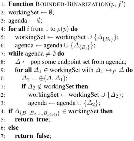
4.3 Bounded binarization algorithm
The adjacency-based binarization algorithm is given in Figure 2. It starts with a working set contain-ing the endpoint sets correspondcontain-ing to each non-terminal occurrence in the input productionp.
Re-ductions ofpare only explored for nonterminal
oc-currences whose endpoint sets are adjacent for the target fan-outf0, since reductions not meeting this
constraint would produce productions with fan-out greater thanf0. Each reduction explored by the
al-gorithm produces a new endpoint set, associated to the fresh nonterminal that it introduces, and this new endpoint set is added to the working set and poten-tially used in further reductions.
From the definition of the adjacency relation↔f, it follows that at lines 9 and 10 of BOUNDED
-BINARIZATION we only pick up reductions for p
that do not exceed the fan-out bound of f0. This
implies soundness for our algorithm. Completeness means that the algorithm fails only if there exists no binarization forpof fan-out not greater thanf0. This
1: FunctionBOUNDED-BINARIZATION(p,f0) 2: workingSet← ∅;
3: agenda← ∅;
4: for allifrom1toρ(p)do
5: workingSet←workingSet∪ {∆{Bi}};
6: agenda←agenda∪ {∆{Bi}}; 7: whileagenda6=∅do
8: ∆←pop some endpoint set from agenda;
9: for all∆1 ∈workingSet with∆1 ↔f0 ∆do
10: ∆2=⊕(∆,∆1);
11: if∆2∈/workingSetthen
12: workingSet←workingSet∪ {∆2}; 13: agenda←agenda∪ {∆2};
14: if∆{B1,B2,...,Bρ(p))} ∈workingSetthen 15: return true;
16: else
[image:5.612.318.539.59.291.2]17: return false;
Figure 2: Algorithm to compute a bounded binarization
property is intuitive if one observes that our algo-rithm is a specialization of standard algoalgo-rithms for the computation of the closure of binary relations. A formal proof of this fact is rather long and te-dious, and will not be reported here. We notice that there is a very close similarity between algorithm BOUNDED-BINARIZATION and the deduction
pro-cedure proposed by Shieber et al. (1995) for parsing. We discuss this more at length in Section 5.
Note that we have expressed the algorithm as a decision function that will return true if there exists a binarization ofpwith fan-out not greater thanf0,
and false otherwise. However, the algorithm can easily be modified to return a reduction producing such a binarization, by adding to each endpoint set
∆ ∈ workingSet two pointers to the adjacent end-point sets that were used to obtain it. If the algorithm is successful, the tree obtained by following these pointers from the final endpoint set∆{B1,...,Bρ(p)} ∈
workingSet gives us a tree of reductions that will produce a binarization ofpwith fan-out not greater thanf0, where each node labeled with the set∆{Bi} corresponds to the nonterminal Bi, and nodes
4.4 Implementation
In order to implement BOUNDED-BINARIZATION,
we can represent endpoint sets in a canonical way as2f0-tuples of integer positions in ascending order,
and with some special null value used to fill posi-tions for endpoint sets with fan-out strictly smaller thanf0. We will assume that the concrete null value
is larger than any other integer.
We also need to provide some appropriate repre-sentation for the set workingSet, in order to guar-antee efficient performance for the membership test and the insertion operation. Both operations can be implemented in constant time if we represent work-ingSet as an(2×f0)-dimensional table with Boolean
entries. Each dimension is indexed by values in [0, n]plus our special null value; herenis the length
of the stringσN(p), and thusn=O(|p|). However, this has the disadvantage of using space Θ(n2f0), even in case workingSet is sparse, and is affordable only for quite small values off0. Alternatively, we
can more compactly represent workingSet as a trie data structure. This representation has size certainly smaller than2f0×q, whereq is the size of the set
workingSet. However, both membership and inser-tion operainser-tions take now an amount of timeO(2f0).
We now analyse the time complexity of algorithm BOUNDED-BINARIZATIONfor inputspandf0. We
first focus on the while-loop at lines 7 to 13. As already observed, the number of possible endpoint sets is bounded byO(n2f0). Furthermore, because
of the test at line 11, no endpoint set is ever inserted into the agenda variable more than once in a sin-gle run of the algorithm. We then conclude that our while-loop cycles a number of timesO(n2f0).
We now focus on the choice of the endpoint set
∆1in the inner for-loop at lines 9 to 13. Let us fix∆
as in line 8. It is not difficult to see that any∆1with ∆1 ↔f0 ∆must satisfy
ϕ(∆) +ϕ(∆1)− |∆∩∆1| ≤ f0. (1)
LetI ⊆ ∆, and consider all endpoint sets∆1 with ∆∩∆1 =I. Given (1), we also have
ϕ(∆1) ≤ f0+|I| −ϕ(∆). (2)
This means that, for each ∆ coming out of the agenda, at line 9 we can choose all endpoint sets∆1
such that ∆1 ↔f0 ∆ by performing the following steps:
• arbitrarily choose a setI ⊆∆;
• choose endpoints in set∆1\Isubject to (2);
• test whether ∆1 belongs to workingSet and
whether∆,∆1do not overlap.
We claim that, in the above steps, the number of involved endpoints does not exceed 3f0. To
see this, we observe that from (2) we can derive
|I| ≥ ϕ(∆) + ϕ(∆1) − f0. The total number
of (distinct) endpoints in a single iteration step is
e = 2ϕ(∆) + 2ϕ(∆1)− |I|. Combining with the
above inequality we have
e ≤ 2ϕ(∆) + 2ϕ(∆1)−ϕ(∆)−ϕ(∆1) +f0
= ϕ(∆) +ϕ(∆1) +f0 ≤ 3f0,
as claimed. Since each endpoint takes values in the set [0, n], we have a total of O(n3f0) different
choices. For each such choice, we need to clas-sify an endpoint as belonging to either∆\I,∆1\I,
or I. This amounts to an additional O(33f0) dif-ferent choices. Overall, we have a total number of
O((3n)3f0)different choices. For each such choice, the test for membership in workingSet for∆1 takes
constant time in case we use a multi-dimensional ta-ble, or else O(|p|) in case we use a trie. The ad-jacency test and the merge operations can easily be carried out in timeO(|p|).
Putting all of the above observations together, and using the already observed fact that n = O(|p|),
we can conclude that the total amount of time re-quired by the while-loop at lines 7 to 13 is bounded byO(|p| ·(3|p|)3f0), both under the assumption that
workingSet is represented as a multi-dimensional ta-ble or as a trie. This is also a bound on the running time of the whole algorithm.
4.5 Minimal binarization of a complete LCFRS
The algorithm defined in Section 4.3 can be used to binarize an LCFRS in such a way that each rule in the resulting binarization has the minimum pos-sible fan-out. This can be done by applying the BOUNDED-BINARIZATION algorithm to each
1: FunctionMINIMAL-BINARIZATION(G) 2: pb =∅ {Set of binarized productions}
3: for allproductionpofGdo 4: f0=fan-out(p);
5: while not BOUNDED-BINARIZATION(p, f0) do
6: f0 =f0+ 1;
7: add result of BOUNDED-BINARIZATION(p, f0) to pb; {We obtain the tree from BOUNDED-BINARIZATION as explained in
Section 4.3 and use it to binarizep} 8: return pb;
Figure 3: Minimal binarization by sequential search
boundf0 for which this algorithm finds a
binariza-tion. For a production with rank r and fan-outf, we know that this optimal value of f0 must be in
the interval [f,d2re ·f] because binarizing a
pro-duction cannot reduce its fan-out, and the NAIVE
-BINARIZATION algorithm seen in Section 4.1 can
binarize any production by increasing fan-out to
dr2e ·f in the worst case.
The simplest way of finding out the optimal value off0 for each production is by a sequential search
starting withϕ(p)and going upwards, as in the
algo-rithm in Figure 3. Note that the upper bounddr2e ·f
that we have given forf0 guarantees that the
while-loop in this algorithm always terminates.
In the worst case, we may needf ·(dr2e −1) + 1
executions of the BOUNDED-BINARIZATION
algo-rithm to find the optimal binarization of a production inG. This complexity can be reduced by changing
the strategy to search for the optimalf0: for
exam-ple, we can perform a binary search within the inter-val[f,dr2e ·f], which lets us find the optimal
bina-rization inblog(f·(dr2e −1) + 1)c+ 1executions of BOUNDED-BINARIZATION. However, this will not
result in a practical improvement, since BOUNDED
-BINARIZATIONis exponential in the value off0and the binary search will require us to run it on val-ues off0 larger than the optimal in most cases. An
intermediate strategy between the two is to apply exponential backoff to try the sequence of values
f−1+2i(fori= 0,1,2. . .). When we find the first isuch that BOUNDED-BINARIZATIONdoes not fail,
ifi > 0, we apply the same strategy to the interval
[f−1+2i−1, f−2+2i], and we repeat this method to shrink the interval until BOUNDED-BINARIZATION
does not fail for i = 0, giving us our optimal f0.
With this strategy, the amount of executions of the algorithm that we need in the worst case is
1
2(dlog(ω)e+dlog(ω)e2) + 1,
whereω = f ·(dr
2e −1) + 1, but we avoid using
unnecessarily large values off0.
5 Discussion
To conclude this paper, we now discuss a number of aspects of the results that we have presented, includ-ing various other pieces of research that are particu-larly relevant to this paper.
5.1 The tradeoff between rank and fan-out
The algorithm introduced in this paper can be used to transform an LCFRS into an equivalent form with rank 2. This will result into a more effi-ciently parsable LCFRS, since rank exponentially affects parsing complexity. However, we must take into account that parsing complexity is also influ-enced by fan-out. Our algorithm guarantees a min-imal increase in fan-out. In practical cases it seems such an increase is quite small. For example, in the context of dependency parsing, both G´omez-Rodr´ıguez et al. (2009) and Kuhlmann and Satta (2009) show that all the structures in several well-known non-projective dependency treebanks are bi-narizable without any increase in their fan-out.
More in general, it has been shown by Seki et al. (1991) that parsing of LCFRS can be carried out in time O(n|pM|), where n is the length of the input string andpM is the production in the grammar with largest size.3Thus, there may be cases in which one
has to find an optimal tradeoff between rank and fan-out, in order to minimize the size ofpM. This re-quires some kind of Viterbi search over the space of all possible binarizations, constructed as described at the end of Subsection 4.3, for some appropriate value of the fan-outf0.
3The result has been shown for the formalism of multiple
5.2 Extension to general LCFRS
This paper has focussed on string-based LCFRS. As discussed in Vijay-Shanker et al. (1987), LCFRS provide a more general framework where the pro-ductions are viewed as generating a set of abstract
derivationtrees. These trees can be used to specify how structures other than tuples of strings are com-posed. For example, LCFRS derivation trees can be used to specify how the elementary trees of a Tree Adjoining Grammar can be composed to produced derived tree. However, the results in this paper also apply to non-string-based LCFRS, since by limit-ing attention to the terminal strlimit-ing yield of whatever structures are under consideration, the composition operations can be defined using the string-based ver-sion of LCFRS that is discussed here.
5.3 Similar algorithmic techniques
The NAIVE-BINARIZATIONalgorithm given in
Fig-ure 1 is not novel to this paper: it is similar to an algorithm developed in Melamed et al. (2004) for generalized multitext grammars, a formalism weakly equivalent to LCFRS that has been intro-duced for syntax-based machine translation. How-ever, the grammar produced by our algorithm has optimal (minimal) fan-out. This is an important im-provement over the result in (Melamed et al., 2004), as this quantity enters into the parsing complexity of both multitext grammars and LCFRS as an expo-nential factor, and therefore must be kept as low as possible to ensure practically viable parsing.
Rank reduction is also investigated in Nesson et al. (2008) for synchronous tree-adjoining gram-mars, a synchronous rewriting formalism based on tree-adjoining grammars Joshi and Schabes (1992). In this case the search space of possible reductions is strongly restricted by the tree structures specified by the formalism, resulting in simplified computa-tion for the reduccomputa-tion algorithms. This feature is not present in the case of LCFRS.
There is a close parallel between the technique used in the MINIMAL-BINARIZATION algorithm
and deductive parsing techniques as proposed by Shieber et al. (1995), that are usually implemented by means of tabular methods. The idea of exploit-ing tabular parsexploit-ing in production factorization was first expressed in Zhang et al. (2006). In fact, the
particular approach presented here has been used to improve efficiency of parsing algorithms that use discontinuous syntactic models, in particular, non-projective dependency grammars, as discussed in G´omez-Rodr´ıguez et al. (2009).
5.4 Open problems
The bounded binarization algorithm that we have presented has exponential run-time in the value of the input fan-out boundf0. It remains an open
ques-tion whether the bounded binarizaques-tion problem for LCFRS can be solved in deterministic polynomial time. Even in the restricted case off0 = ϕ(p), that
is, when no increase in the fan-out of the input pro-duction is allowed, we do not know whetherpcan be
binarized using only deterministic polynomial time in the value ofp’s fan-out. However, our bounded
binarization algorithm shows that the latter problem can be solved in polynomial time when the fan-out of the input LCFRS is bounded by some constant.
Whether the bounded binarization problem can be solved in polynomial time in the value of the input bound f0 is also an open problem in the
re-stricted case of synchronous context-free grammars, a special case of an LCFRS of fan-out two with a strict separation between the two components of each nonterminal in the right-hand side of a produc-tion, as discussed in the introduction. An interesting analysis of this restricted problem can be found in Gildea and Stefankovic (2007).
References
David Chiang. 2007. Hierarchical
phrase-based translation. Computational Linguistics, 33(2):201–228.
Daniel Gildea and Daniel Stefankovic. 2007. Worst-case synchronous grammar rules. InHuman Lan-guage Technologies 2007: The Conference of the North American Chapter of the Association for Computational Linguistics; Proceedings of the Main Conference, pages 147–154. Association for Computational Linguistics, Rochester, New York.
Carlos G´omez-Rodr´ıguez, David J. Weir, and John Carroll. 2009. Parsing mildly non-projective de-pendency structures. InTwelfth Conference of the European Chapter of the Association for Compu-tational Linguistics (EACL). To appear.
A. K. Joshi and Y. Schabes. 1992. Tree adjoining grammars and lexicalized grammars. In M. Nivat and A. Podelsky, editors,Tree Automata and Lan-guages. Elsevier, Amsterdam, The Netherlands. Marco Kuhlmann and Joakim Nivre. 2006. Mildly
non-projective dependency structures. In 21st International Conference on Computational Lin-guistics and 44th Annual Meeting of the Asso-ciation for Computational Linguistics (COLING-ACL), Main Conference Poster Sessions, pages 507–514. Sydney, Australia.
Marco Kuhlmann and Giorgio Satta. 2009. Tree-bank grammar techniques for non-projective de-pendency parsing. In Twelfth Conference of the European Chapter of the Association for Compu-tational Linguistics (EACL). To appear.
I. Dan Melamed, Benjamin Wellington, and Gior-gio Satta. 2004. Generalized multitext gram-mars. In42nd Annual Meeting of the Association for Computational Linguistics (ACL), pages 661– 668. Barcelona, Spain.
Rebecca Nesson, Giorgio Satta, and Stuart M. Shieber. 2008. Optimal k-arization of
syn-chronous tree-adjoining grammar. InProceedings of ACL-08: HLT, pages 604–612. Association for Computational Linguistics, Columbus, Ohio. A. Nijholt. 1980. Context-Free Grammars:
Cov-ers, Normal Forms, and Parsing, volume 93. Springer-Verlag, Berlin, Germany.
Owen Rambow and Giorgio Satta. 1999. Indepen-dent parallelism in finite copying parallel rewrit-ing systems. Theoretical Computer Science, 223(1–2):87–120.
Hiroyuki Seki, Takashi Matsumura, Mamoru Fujii, and Tadao Kasami. 1991. On Multiple Context-Free Grammars. Theoretical Computer Science, 88(2):191–229.
Stuart M. Shieber, Yves Schabes, and Fernando Pereira. 1995. Principles and implementation of deductive parsing. Journal of Logic Program-ming, 24(1–2):3–36.
Takeaki Uno and Mutsunori Yagiura. 2000. Fast al-gorithms to enumerate all common intervals of two permutations. Algorithmica, 26(2):290–309. K. Vijay-Shanker, David J. Weir, and Aravind K.
Joshi. 1987. Characterizing structural descrip-tions produced by various grammatical for-malisms. In25th Annual Meeting of the Associ-ation for ComputAssoci-ational Linguistics (ACL), pages 104–111. Stanford, CA, USA.
Benjamin Wellington, Sonjia Waxmonsky, and I. Dan Melamed. 2006. Empirical lower bounds on the complexity of translational equivalence. In
21st International Conference on Computational Linguistics and 44th Annual Meeting of the Asso-ciation for Computational Linguistics (COLING-ACL), pages 977–984. Sydney, Australia.
Hao Zhang, Daniel Gildea, and David Chiang. 2008. Extracting synchronous grammar rules from word-level alignments in linear time. In
22nd International Conference on Computational Linguistics (Coling), pages 1081–1088. Manch-ester, England, UK.