Proceedings of NAACL-HLT 2018, pages 2092–2102
Factors Influencing the Surprising Instability of Word Embeddings
Laura Wendlandt, Jonathan K. Kummerfeld and Rada Mihalcea Computer Science & Engineering
University of Michigan, Ann Arbor
{wenlaura,jkummerf,mihalcea}@umich.edu
Abstract
Despite the recent popularity of word embed-ding methods, there is only a small body of work exploring the limitations of these repre-sentations. In this paper, we consider one as-pect of embedding spaces, namely their sta-bility. We show that even relatively high fre-quency words (100-200 occurrences) are often unstable. We provide empirical evidence for how various factors contribute to the stability of word embeddings, and we analyze the ef-fects of stability on downstream tasks.
1 Introduction
Word embeddings are low-dimensional, dense vector representations that capture semantic prop-erties of words. Recently, they have gained tremendous popularity in Natural Language Pro-cessing (NLP) and have been used in tasks as diverse as text similarity (Kenter and De Rijke, 2015), part-of-speech tagging (Tsvetkov et al., 2016), sentiment analysis (Faruqui et al., 2015), and machine translation (Mikolov et al., 2013a). Although word embeddings are widely used across NLP, their stability has not yet been fully evaluated and understood. In this paper, we ex-plore the factors that play a role in the stability of word embeddings, including properties of the data, properties of the algorithm, and properties of the words. We find that word embeddings exhibit substantial instabilities, which can have implica-tions for downstream tasks.
Using the overlap between nearest neighbors in an embedding space as a measure of stability (see section 3 below for more information), we ob-serve that many common embedding spaces have large amounts of instability. For example, Figure1 shows the instability of the embeddings obtained by trainingword2vecon the Penn Treebank (PTB) (Marcus et al., 1993). As expected, lower quency words have lower stability and higher
fre-20 24 28 212 216
Frequency of Word in PTB (log scale)
10075 50
25
10
5
2
% Stability (log scale)
1e-04 1e-03 1e-02 1e-01 1
% Words in Particular Frequency Bucket
[image:1.595.309.529.207.371.2](log scale)
Figure 1: Stability ofword2vec as a property of fre-quency in the PTB. Stability is measured across ten randomized embedding spaces trained on the training portion of the PTB (determined using language model-ing splits (Mikolov et al.,2010)). Each word is placed in a frequency bucket (x-axis), and each column (fre-quency bucket) is normalized.
quency words have higher stability. What is sur-prising however about this graph is the medium-frequency words, which show huge variance in stability. This cannot be explained by frequency, so there must be other factors contributing to their instability.
In the following experiments, we explore which factors affect stability, as well as how this stability affects downstream tasks that word embeddings are commonly used for. To our knowledge, this is the first study comprehensively examining the factors behind instability.
2 Related Work
There has been much recent interest in the applica-tions of word embeddings, as well as a small, but growing, amount of work analyzing the properties of word embeddings.
word2vec (Mikolov et al., 2013b), and GloVe (Pennington et al.,2014). Various aspects of the embedding spaces produced by these algorithms have been previously studied. Particularly, the ef-fect of parameter choices has a large impact on how all three of these algorithms behave (Levy et al.,2015). Further work shows that the param-eters of the embedding algorithmword2vec influ-ence the geometry of word vectors and their con-text vectors (Mimno and Thompson,2017). These parameters can be optimized; Hellrich and Hahn (2016) posit optimal parameters for negative sam-pling and the number of epochs to train for. They also demonstrate that in addition to parameter set-tings, word properties, such as word ambiguity, af-fect embedding quality.
In addition to exploring word and algorithmic parameters, concurrent work by Antoniak and Mimno (2018) evaluates how document properties affect the stability of word embeddings. We also explore the stability of embeddings, but focus on a broader range of factors, and consider the effect of stability on downstream tasks. In contrast, Anto-niak and Mimno focus on using word embeddings to analyze language (e.g.,Garg et al.,2018), rather than to perform tasks.
At a higher level of granularity, Tan et al. (2015) analyze word embedding spaces by comparing two spaces. They do this by linearly transforming one space into another space, and they show that words have different usage properties in different domains (in their case, Twitter and Wikipedia).
Finally, embeddings can be analyzed using second-order properties of embeddings (e.g., how a word relates to the words around it). Newman-Griffis and Fosler-Lussier (2017) validate the use-fulness of second-order properties, by demonstrat-ing that embedddemonstrat-ings based on second-order prop-erties perform as well as the typical first-order em-beddings. Here, we use second-order properties of embeddings to quantify stability.
3 Defining Stability
We definestabilityas the percent overlap between nearest neighbors in an embedding space.1 Given a wordW and two embedding spaces A andB, take the ten nearest neighbors of W in both A and B. Let the stability of W be the percent
1This metric is concurrently explored in work by Anto-niak and Mimno (2018).
Model 1 Model 2 Model 3 metropolitan ballet national national metropolitan ballet
egyptian bard metropolitan
rhode chicago institute
society national glimmerglass
debut state egyptian
folk exhibitions intensive
reinstallation society jazz chairwoman whitney state
[image:2.595.309.525.61.217.2]philadelphia rhode exhibitions
Table 1: Top ten most similar words for the word
inter-nationalin three randomly intializedword2vecmodels
trained on the NYT Arts Domain. Words in all three lists are in bold; words in only two of the lists are itali-cized.
overlap between these two lists of nearest neigh-bors. 100% stability indicates perfect agreement between the two embedding spaces, while 0% sta-bility indicates complete disagreement. In order to find the ten nearest neighbors of a wordW in an embedding spaceA, we measure distance between words using cosine similarity.2 This definition of stability can be generalized to more than two em-bedding spaces by considering the average overlap between two sets of embedding spaces. LetXand Y be two sets of embedding spaces. Then, for ev-ery pair of embedding spaces(x, y), wherex∈X andy∈Y, take the ten nearest neighbors ofW in bothxandyand calculate percent overlap. Let the stability be the average percent overlap over every pair of embedding spaces(x, y).
Consider an example using this metric. Ta-ble1 shows the top ten nearest neighbors for the
word international in three randomly initialized
word2vec embedding spaces trained on the NYT
Arts domain (see Section 4.3 for a description of this corpus). These models share some simi-lar words, such asmetropolitanandnational, but there are also many differences. On average, each pair of models has four out of ten words in com-mon, so the stability ofinternationalacross these three models is 40%.
The idea of evaluating ten best options is also found in other tasks, like lexical substitution (e.g., McCarthy and Navigli, 2007) and word
100
80
60
40
20
0
% Stability
110
50
100
200
800
max
Frequency in Training Corpus (approx. log-based scale)
0.0 0.2 0.4 0.6 0.8 1.0
% Words in Particular Frequency Bucket
9998 1024 32 2 9998 1024 32 2 9998 1024 32 2 9998 1024 32 2 9998 1024 32 2 9998 1024 32 2
[image:3.595.82.293.65.375.2]# of Nearest Neighbors (log scale)
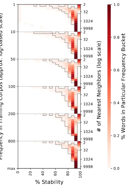
Figure 2: Stability of GloVe on the PTB. Stability is measured across ten randomized embedding spaces trained on the training data of the PTB (determined us-ing language modelus-ing splits (Mikolov et al.,2010)). Each word is placed in a frequency bucket (left y-axis) and stability is determined using a varying number of nearest neighbors for each frequency bucket (right y-axis). Each row is normalized, and boxes with more than 0.01 of the row’s mass are outlined.
tion (e.g., Garimella et al., 2017), where the top ten results are considered in the final evaluation metric. To give some intuition for how changing the number of nearest neighbors affects our stabil-ity metric, consider Figure 2. This graph shows how the stability of GloVe changes with the fre-quency of the word and the number of neighbors used to calculate stability; please see the figure caption for a more detailed explanation of how this graph is structured. Within each frequency bucket, the stability is consistent across varying numbers of neighbors. Ten nearest neighbors per-forms approximately as well as a higher number of nearest neighbors (e.g., 100). We see this pat-tern for low frequency words as well as for high frequency words. Because the performance does not change substantially by increasing the num-ber of nearest neighbors, it is computationally less intensive to use a small number of nearest
neigh-bors. We choose ten nearest neighbors as our met-ric throughout the rest of the paper.
4 Factors Influencing Stability
As we saw in Figure1, embeddings are sometimes surprisingly unstable. To understand the factors behind the (in)stability of word embeddings, we build a regression model that aims to predict the stability of a word given: (1) properties related to the word itself; (2) properties of the data used to train the embeddings; and (3) properties of the al-gorithm used to construct these embeddings. Us-ing this regression model, we draw observations about factors that play a role in the stability of word embeddings.
4.1 Methodology
We use ridge regression to model these various factors (Hoerl and Kennard, 1970). Ridge re-gression regularizes the magnitude of the model weights, producing a more interpretable model than non-regularized linear regression. This regu-larization mitigates the effects of multicollinearity (when two features are highly correlated). Specif-ically, given N ground-truth data points with M extracted features per data point, letxn ∈ R1×M
be the features for samplenand lety∈R1×N be
the set of labels. Then, ridge regression learns a set of weightsw∈R1×M by minimizing the least squares function withl2regularization, whereλis a regularization constant:
L(w) = 1 2
N
X
n=1
(yn−w>xn)2+λ
2||w||
2
We set λ = 1. In addition to ridge regression, we tried non-regularized linear regression. We ob-tained comparable results, but many of the weights were very large or very small, making them hard to interpret.
The goodness of fit of a regression model is measured using the coefficient of determination R2. This measures how much variance in the de-pendent variableyis captured by the independent variablesx. A model that always predicts the ex-pected value ofy, regardless of the input features, will receive anR2score of 0. The highest possible R2 score is 1, and theR2score can be negative.
words across various combinations of two embed-ding spaces. Specifically, given a wordW and two embedding spaces A and B, we encode proper-ties of the word W, as well as properties of the
datasetsand thealgorithmsused to train the
em-bedding spacesAandB. The target value associ-ated with this features is the stability of the word W across embedding spacesAandB. We repeat this process for more than 2,500 words, several datasets, and three embedding algorithms.
Specifically, we consider all the words present in all seven of the data domains we are using (see Section4.3), 2,521 words in total. Using the ture categories described below, we generate a fea-ture vector for each unique word, dataset, algo-rithm, and dimension size, resulting in a total of 27,794,025 training instances. To get good aver-age estimates for each embedding algorithm, we train each embedding space five times, random-ized differently each time (this does not apply to PPMI, which has no random component). We then train a ridge regression model on these in-stances. The model is trained to predict the stabil-ity of wordW across embedding spacesAandB (whereAandB are not necessarily trained using the same algorithm, parameters, or training data). Because we are using this model to learn associa-tions between certain features and stability, no test data is necessary. The emphasis is on the model it-self, not on the model’s performance on a specific task.
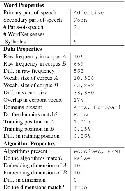
We describe next each of the three main cate-gories of factors examined in the model. An ex-ample of these features is given in Table2. 4.2 Word Properties
We encode several features that capture attributes of the wordW. First, we use the primary and sec-ondary part-of-speech (POS) of the word. Both of these are represented as bags-of-words of all possible POS, and are determined by looking at the primary (most frequent) and secondary (sec-ond most frequent) POS of the word in the Brown corpus3(Francis and Kucera,1979). If the word is not present in the Brown corpus, then all of these POS features are set to zero.
To get a coarse-grained representation of the
3Here, we use the universal tagset, which consists of twelve possible POS: adjective, adposition, adverb, conjunc-tion, determiner / article, noun, numeral, particle, pronoun, verb, punctuation mark, and other (Petrov et al.,2012).
Word Properties
Primary part-of-speech Adjective
Secondary part-of-speech Noun
# Parts-of-speech 2
# WordNet senses 3
Syllables 5
Data Properties
Raw frequency in corpusA 106
Raw frequency in corpusB 669
Diff. in raw frequency 563
Vocab. size of corpusA 10,508
Vocab. size of corpusB 43,888
Diff. in vocab. size 33,380
Overlap in corpora vocab. 17%
Domains present Arts, Europarl
Do the domains match? False
Training position inA 1.02%
Training position inB 0.15%
Diff. in training position 0.86%
Algorithm Properties
Algorithms present word2vec, PPMI
Do the algorithms match? False
Embedding dimension ofA 100
Embedding dimension ofB 100
Diff. in dimension 0
[image:4.595.309.524.60.388.2]Do the dimensions match? True
Table 2: Consider the wordinternational in two em-bedding spaces. Suppose emem-bedding spaceAis trained
using word2vec (embedding dimension 100) on the NYT Arts domain, and embedding spaceB is trained using PPMI (embedding dimension 100) on Europarl. This table summarizes the resulting features for this word across the two embedding spaces.
polysemy of the word, we consider the number of different POS present. For a finer-grained repre-sentation, we use the number of different Word-Net senses associated with the word (Miller,1995; Fellbaum,1998).
We also consider the number of syllables in a word, determined using the CMU Pronuncing Dic-tionary (Weide, 1998). If the word is not present in the dictionary, then this is set to zero.
4.3 Data Properties
Vocab. Num. Tokens / Dataset Sentences Size Vocab. Size
NYT US 13,923 5,787 64.37
NYT NY 36,792 11,182 80.41
NYT Business 21,048 7,212 75.96
NYT Arts 28,161 10,508 65.29
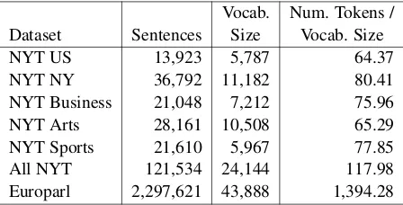
[image:5.595.75.299.62.176.2]NYT Sports 21,610 5,967 77.85 All NYT 121,534 24,144 117.98 Europarl 2,297,621 43,888 1,394.28
Table 3: Dataset statistics.
domains 1-5 (denoted “All NYT”), and (7) All of English Europarl. Table 3 shows statistics about these datasets. The first five domains are chosen because they are the top five most common cate-gories of news articles present in the NYT corpus. They are smaller than “All NYT” and Europarl, and they have a narrow topical focus. The “All NYT” domain is more diverse topically and larger than the first five domains. Finally, the Europarl domain is the largest domain, and it is focused on a single topic (European Parliamentary politics). These varying datasets allow us to consider how data-dependent properties affect stability.
We use several features related to domain. First, we consider the raw frequency of wordW in both the domain of data used for embedding space A and the domain of data for space B. To make our regression model symmetric, we effectively encode three features: the higher raw frequency (between the two), the lower raw frequency, and the absolute difference in raw frequency.
We also consider the vocabulary size of each corpus (again, symmetrically) and the percent overlap between corpora vocabulary, as well as the domain of each of the two corpora, represented as a bag-of-words of domains. Finally, we con-sider whether the two corpora are from the same domain.
Our final data-level features explore the role of curriculum learning in stability. It has been posited that the order of the training data affects the performance of certain algorithms, and previ-ous work has shown that for some neural network-based tasks, a good training data order (curricu-lum learning strategy) can improve performance (Bengio et al., 2009). Curriculum learning has been previously explored for word2vec, where it has been found that optimizing training data order can lead to small improvements on common NLP tasks (Tsvetkov et al.,2016). Of the embedding
algorithms we consider, curriculum learning only affects word2vec. Because GloVe and PPMI use the data to learn a complete matrix before build-ing embeddbuild-ings, the order of the trainbuild-ing data will not affect their performance. To measure the ef-fects of training data order, we include as features the first appearance of wordW in the dataset for embedding spaceAand the first appearance ofW in the dataset for embedding spaceB(represented as percentages of the total number of training sen-tences)4. We further include the absolute differ-ence between these percentages.
4.4 Algorithm Properties
In addition to word and data properties, we encode features about the embedding algorithms. These include the different algorithms being used, as well as the different parameter settings of these algorithms. Here, we consider three embedding algorithms, word2vec, GloVe, and PPMI. The choice of algorithm is represented in our feature vector as a bag-of-words.
PPMI creates embeddings by first building a positive pointwise mutual information word-context matrix, and then reducing the dimension-ality of this matrix using SVD (Bullinaria and Levy,2007). A more recent word embedding al-gorithm, word2vec (skip-gram model) (Mikolov et al., 2013b) uses a shallow neural network to learn word embeddings by predicting context words. Another recent method for creating word embeddings, GloVe, is based on factoring a matrix of ratios of co-occurrence probabilities ( Penning-ton et al.,2014).
For each algorithm, we choose common param-eter settings. Forword2vec, two of the parameters that need to be chosen are window size and mini-mum count. Window size refers to the maximini-mum distance between the current word and the pre-dicted word (e.g., how many neighboring words to consider for each target word). Any word appear-ing less than the minimum count number of times in the corpus is discarded and not considered in the
word2vec algorithm. For both of these features,
we choose standard parameter settings, namely, a window size of 5 and a minimum count of 5. For GloVe, we also choose standard parameters. We
Feature Weight Lower training data position of wordW -1.52
Higher training data position ofW -1.49
Primary POS = Numeral 1.12
Primary POS = Other -1.08
Primary POS = Punctuation mark -1.02 Overlap between corpora vocab. 1.01 Primary POS = Adjective -0.92 Primary POS = Adposition -0.92 Do the two domains match? 0.91
Primary POS = Verb -0.88
Primary POS = Conjunction -0.84
Primary POS = Noun -0.81
Primary POS = Adverb -0.79 Do the two algorithms match? 0.78 Secondary POS = Pronoun 0.62 Primary POS = Determiner -0.48 Primary POS = Particle -0.44 Secondary POS = Particle 0.36 Secondary POS = Other 0.28 Primary POS = Pronoun -0.26 Secondary POS = Verb -0.25 Number ofword2vecembeddings -0.21 Secondary POS = Adverb 0.15 Secondary POS = Determiner 0.14 Number of NYT Arts Domain -0.14 Number of NYT All Domain 0.14 Number of GloVe embeddings 0.13
[image:6.595.77.283.62.421.2]Number of syllables -0.11
Table 4: Regression weights with a magnitude greater than 0.1, sorted by magnitude.
use 50 iterations of the algorithm for embedding dimensions less than 300, and 100 iterations for higher dimensions.
We also add a feature reflecting the embedding dimension, namely one of five embedding dimen-sions: 50, 100, 200, 400, or 800.
5 Lessons Learned: What Contributes to the Stability of an Embedding
Overall, the regression model achieves a coeffi-cient of determination (R2) score of 0.301 on the training data, which indicates that the regression has learned a linear model that reasonably fits the training data given. Using the regression model, we can analyze the weights corresponding to each of the features being considered, shown in Table4. These weights are difficult to interpret, because features have different distributions and ranges. However, we make several general observations about the stability of word embeddings.
Observation 1. Curriculum learning is
impor-100 10
1 0.1 0.01 0
Position in Training Data (%, log scale)
100 75 50 25
10 5
2 0
% Stability (log scale)
0.0 0.1 0.2 0.3 0.4 0.5
% Vocabulary
(a)word2vec
100 10
1 0.1 0.01 0
Position in Training Data (%, log scale)
100 75 50 25
10 5
2 0
% Stability (log scale)
0.0 0.6 1.2 1.8 2.4 3.0 3.6
% Vocabulary
[image:6.595.83.283.64.426.2](b) GloVe
Figure 3: Stability of both word2vec and GloVe as properties of the starting word position in the training data of the PTB. Stability is measured across ten ran-domized embedding spaces trained on the training data of the PTB (determined using language modeling splits
(Mikolov et al.,2010)). Boxes with more than 0.02%
of the total vocabulary mass are outlined.
tant. This is evident because the top two features (by magnitude) of the regression model capture where the word first appears in the training data. Figure3shows trends between training data posi-tion and stability in the PTB. This figure contrasts
word2vecwith GloVe (which is order invariant).
To further understand the effect of curriculum learning on the model, we train a regression model with all of the features except the curriculum learning features. This model achieves an R2 score of 0.291 (compared to the full model’s score of 0.301). This indicates that curriculum learning is a factor in stability.
[image:6.595.310.534.65.415.2]aver-Primary POS Avg. Stability
Numeral 47%
Verb 31%
Determiner 31%
Adjective 31%
Noun 30%
Adverb 29%
Pronoun 29%
Conjunction 28%
Particle 26%
Adposition 25%
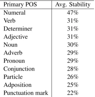
[image:7.595.100.264.62.229.2]Punctuation mark 22%
Table 5: Percent stability broken down by part-of-speech, ordered by decreasing stability.
age stabilities for each primary POS. Here we see that the most stable POS are numerals, verbs, and determiners, while the least stable POS are punc-tuation marks, adpositions, and particles.
Observation 3. Stability within domains is greater than stability across domains. Table4 shows that many of the top factors are domain-related. Figure4 shows the results of the regres-sion model broken down by domain. This figure shows the highest stabilities appearing on the di-agonal of the matrix, where the two embedding spaces both belong to the same domain. The sta-bilities are substantially lower off the diagonal.
Figure 4 also shows that “All NYT” general-izes across the other NYT domains better than Europarl, but not as well as in-domain data (“All NYT” encompasses data from US, NY, Business, Arts, and Sports). This is true even though Eu-roparl is much larger than “All NYT”.
Observation 4. Overall, GloVe is the most sta-ble embedding algorithm. This is particularly apparent when only in-domain data is considered, as in Figure 5. PPMI achieves similar stability, whileword2veclags considerably behind.
To further compare word2vec and GloVe, we look at how the stability of word2vec changes with the frequency of the word and the number of neighbors used to calculate stability. This is shown in Figure6and is directly comparable to Figure2. Surprisingly, the stability ofword2vecvaries sub-stantially with the frequency of the word. For lower-frequency words, as the number of near-est neighbors increases, the stability increases ap-proximately exponentially. For high-frequency words, the lowest and highest number of nearest
NYT US NYT NY NYT Business
NYT Arts
NYT Sports All NYT Europarl
NYT US NYT NY NYT Business NYT Arts NYT Sports All NYT Europarl
18 4.4 21 3.7 4.7 20 2.6 4 2.9 18 2.7 3.6 3 2.6 19
6 11 7.8 6.4 6.1 27 2.6 4 3.2 2.5 2.4 7 30
0
15
30
45
60
75
[image:7.595.310.530.64.226.2]% Stability
Figure 4: Percent stability broken down by domain.
w2v PPMI GloVe
w2v
PPMI
GloVe
29
6.6
52
8.2
11
65
0
15
30
45
60
75
[image:7.595.350.481.270.371.2]% Stability
Figure 5: Percent stability broken down between algo-rithm (in-domain data only).
neighbors show the greatest stability. This is dif-ferent than GloVe, where stability remains reason-ably constant across word frequencies, as shown in Figure2. The behavior we see here agrees with the conclusion of (Mimno and Thompson,2017), who find that GloVe exhibits more well-behaved geometry thanword2vec.
Observation 5. Frequency is not a major factor in stability. To better understand the role that fre-quency plays in stability, we run separate ablation experiments comparing regression models with frequency features to regression models without frequency features. Our current model (using raw frequency) achieves anR2 score of 0.301. Com-parably, a model using the same features, but with normalized instead of raw frequency, achieves a score of 0.303. Removing frequency from either regression model gives a score of 0.301. This indi-cates that frequency is not a major factor in stabil-ity, though normalized frequency is a larger factor than raw frequency.
100
80
60
40
20
0
% Stability
110
50
100
200
800
max
Frequency in Training Corpus (approx. log-based scale)
0.2 0.4 0.6 0.8 1.0
% Words in Particular Frequency Bucket
9998 1024 32 2 9998 1024 32 2 9998 1024 32 2 9998 1024 32 2 9998 1024 32 2 9998 1024 32 2
[image:8.595.290.533.63.224.2]# of Nearest Neighbors (log scale)
Figure 6: Stability ofword2vecon the PTB. Stability is measured across ten randomized embedding spaces trained on the training data of the PTB (determined us-ing language modelus-ing splits (Mikolov et al.,2010)). Each word is placed in a frequency bucket (left y-axis) and stability is determined using a varying number of nearest neighbors for each frequency bucket (right y-axis). Each row is normalized, and boxes with more than 0.01 of the row’s mass are outlined.
a model with only normalized frequency features has an R2 score of 0.0059. This indicates that while frequency is not a major factor in stability, it is also not negligible. As we pointed out in the in-troduction, frequency does correlate with stability (Figure1). However, in the presence of all of these other features, frequency becomes a minor factor.
6 Impact of Stability on Downstream Tasks
Word embeddings are used extensively as the first stage of neural networks throughout NLP. Typi-cally, embeddings are initalized based on a vector trained withword2vec or GloVe and then further modified as part of training for the target task. We study two downstream tasks to see whether stabil-ity impacts performance.
Since we are interested in seeing the impact of
0 10 20 30 40 50 60 70 80 90 100
Word 2 Stability (%)
100 90 80 70 60 50 40 30 20 10 0
Word 1 Stability (%)
0.0 0.1 0.2 0.3 0.4 0.5
[image:8.595.79.292.69.373.2]Average Absolute Error
Figure 7: Absolute error for word similarity.
word vector stability, we choose tasks that have an intuitive evaluation at the word level: word simi-larity and POS tagging.
6.1 Word Similarity
To model word similarity, we use 300-dimensional
word2vecembedding spaces trained on the PTB.
For each pair of words, we take the cosine simi-larity between those words averaged over ten ran-domly initialized embedding spaces.
We consider three datasets for evaluating word similarity: WS353 (353 pairs) (Finkelstein et al., 2001), MTurk287 (287 pairs) (Radinsky et al., 2011), and MTurk771 (771 pairs) (Halawi et al., 2012). For each dataset, we normalize the simi-larity to be in the range[0,1], and we take the
ab-solute difference between our predicted value and the ground-truth value. Figure7shows the results broken down by stability of the two words (we al-ways consider Word 1 to be the more stable word in the pair). Word similarity pairs where one of the words is not present in the PTB are omitted.
We find that these word similarity datasets do not contain a balanced distribution of words with respect to stability; there are substantially more unstable words than there are stable words. How-ever, we still see a slight trend: As the combined stability of the two words increases, the average absolute error decreases, as reflected by the lighter color of the cells in Figure7 while moving away from the (0,0) data point.
6.2 Part-of-Speech Tagging
0 10 20 30 40 50 60 70 80 90 100
% Stability
max 4000 1000 250 60 15 0
Frequency
0.0 0.1 0.2 0.3 0.4 0.5
Avg. POS Tagging Error
(a) POS error probability with fixed vectors.
0 10 20 30 40 50 60 70 80 90 100
% Stability
max 4000 1000 250 60 15 0
Frequency
0.0 0.1 0.2 0.3 0.4 0.5
Avg. POS Tagging Error
(b) POS error probability when vectors may shift in training.
0 10 20 30 40 50 60 70 80 90 100
% Stability
max 4000 1000 250 60 15 0
Frequency
0.0 0.2 0.4 0.6 0.8 1.0
Similarity (0 to 1)
[image:9.595.72.287.65.336.2](c) Cosine similarity between original word vectors and shifted word vectors.
Figure 8: Results for POS tagging. (a) and (b) show average POS tagging error divided by the number of to-kens (darker is more errors) while either keeping word vectors fixed or not during training. (c) shows word vector shift, measured as cosine similarity between ini-tial and final vectors. In all graphs, words are bucketed by frequency and stability.
128-dimensional word embeddings withword2vec
using different random seeds. The LSTM has a single layer and 50-dimensional hidden vectors. Outputs are passed through a tanh layer before classification. To train, we use SGD with a learn-ing rate of 0.1, an input noise rate of 0.1, and re-current dropout of 0.4.
This simple model is not state-of-the-art, scor-ing 95.5% on the development set, but the word vectors are a central part of the model, provid-ing a clear signal of their impact. For each word, we group tokens based on stability and frequency.
Figure8shows the results.5 Fixing the word vec-tors provides a clearer pattern in the results, but also leads to much worse performance: 85.0% on the development set. Based on these results, it seems that training appears to compensate for sta-bility. This hypothesis is supported by Figure8c, which shows the similarity between the original word vectors and the shifted word vectors pro-duced by the training. In general, lower stability words are shifted more during training.
Understanding how the LSTM is changing the input embeddings is useful information for tasks with limited data, and it could allow us to im-prove embeddings and LSTM training for these low-resource tasks.
7 Conclusion and Recommendations
Word embeddings are surprisingly variable, even for relatively high frequency words. Using a re-gression model, we show that domain and part-of-speech are key factors of instability. Downstream experiments show that stability impacts tasks us-ing embeddus-ing-based features, though allowus-ing embeddings to shift during training can reduce this effect. In order to use the most stable embed-ding spaces for future tasks, we recommend ei-ther using GloVe or learning a good curriculum
for word2vectraining data. We also recommend
using in-domain embeddings whenever possible. The code used in the experiments described in this paper is publicly available from http: //lit.eecs.umich.edu/downloads.html.
Acknowledgments
We would like to thank Ben King and David Ju-rgens for helpful discussions about this paper, as well as our anonymous reviewers for useful feed-back. This material is based in part upon work supported by the National Science Foundation (NSF #1344257) and the Michigan Institute for Data Science (MIDAS). Any opinions, findings, and conclusions or recommendations expressed in this material are those of the authors and do not necessarily reflect the views of the NSF or MI-DAS.
References
Maria Antoniak and David Mimno. 2018. Eval-uating the stability of embedding-based word
similarities. Transactions of the Association for
Computational Linguistics (TACL) 6:107–119.
https://transacl.org/ojs/index.php/ tacl/article/view/1202.
Yoshua Bengio, J´erˆome Louradour, Ronan Collobert, and Jason Weston. 2009. Curriculum learning. In Proceedings of the International Conference on
Ma-chine Learning (ICML). pages 41–48. https://
dl.acm.org/citation.cfm?id=1553380.
John A Bullinaria and Joseph P Levy. 2007. Ex-tracting semantic representations from word
co-occurrence statistics: A computational study.
Behavior Research Methods 39(3):510–526.
https://link.springer.com/article/ 10.3758/BF03193020.
Manaal Faruqui, Jesse Dodge, Sujay K Jauhar, Chris Dyer, Eduard Hovy, and Noah A Smith. 2015.
Retrofitting word vectors to semantic lexicons. In
Proceedings of the Conference of the North Amer-ican Chapter of the Association for Computa-tional Linguistics: Human Language
Technolo-gies (NAACL: HLT). pages 1606–1615. http:
//www.aclweb.org/anthology/N15-1184.
Christiane Fellbaum. 1998. WordNet. Wiley Online Library. https:// onlinelibrary.wiley.com/doi/full/ 10.1002/9781405198431.wbeal1285.
Lev Finkelstein, Evgeniy Gabrilovich, Yossi Ma-tias, Ehud Rivlin, Zach Solan, Gadi Wolfman, and Eytan Ruppin. 2001. Placing search in
context: The concept revisited. In
Proceed-ings of the International Conference on World
Wide Web (WWW). pages 406–414. https://
dl.acm.org/citation.cfm?id=372094.
W Nelson Francis and Henry Kucera. 1979. Brown corpus manual. Brown University2.
Nikhil Garg, Londa Schiebinger, Dan Jurafsky, and James Zou. 2018. Word embeddings quan-tify 100 years of gender and ethnic
stereo-types. Proceedings of the National Academy of
Sciences (PNAS)https://doi.org/10.1073/
pnas.1720347115.
Aparna Garimella, Carmen Banea, and Rada Mi-halcea. 2017. Demographic-aware word
associa-tions. InProceedings of the International
Confer-ence on Empirical Methods in Natural Language
Processing (EMNLP). pages 2285–2295. http:
//www.aclweb.org/anthology/D17-1242.
Guy Halawi, Gideon Dror, Evgeniy Gabrilovich, and Yehuda Koren. 2012. Large-scale
learn-ing of word relatedness with constraints. In
Proceedings of the International Conference on
Knowledge Discovery and Data Mining (SIGKDD).
pages 1406–1414. https://dl.acm.org/ citation.cfm?id=2339751.
Johannes Hellrich and Udo Hahn. 2016. Bad company-Neighborhoods in neural embedding spaces
con-sidered harmful. In Proceedings of the
Inter-national Conference on Computational
Linguis-tics (COLING). pages 2785–2796. http://
www.aclweb.org/anthology/C16-1262.
Arthur E Hoerl and Robert W Kennard. 1970. Ridge
regression: Biased estimation for
nonorthog-onal problems. Technometrics 12(1):55–67.
https://amstat.tandfonline.com/doi/ abs/10.1080/00401706.1970.10488634.
Tom Kenter and Maarten De Rijke. 2015. Short
text similarity with word embeddings. In
Pro-ceedings of the 24th ACM International on Con-ference on Information and Knowledge
Manage-ment (CIKM). pages 1411–1420. https://
dl.acm.org/citation.cfm?id=2806475. Philipp Koehn. 2005. Europarl: A parallel corpus for
statistical machine translation. InMachine
Transla-tion Summit X. volume 5, pages 79–86.
Omer Levy, Yoav Goldberg, and Ido Dagan. 2015. Im-proving distributional similarity with lessons learned
from word embeddings.Transactions of the
Associ-ation for ComputAssoci-ational Linguistics (TACL)3:211–
225. https://www.transacl.org/ojs/ index.php/tacl/article/view/570.
Mitchell P Marcus, Mary Ann Marcinkiewicz, and Beatrice Santorini. 1993. Building a large
anno-tated corpus of English: The Penn treebank.
Com-putational Linguistics19(2):313–330. https://
dl.acm.org/citation.cfm?id=972475. Diana McCarthy and Roberto Navigli. 2007.
Semeval-2007 task 10: English lexical substitution task.
In Proceedings of the International Workshop on
Semantic Evaluations (SemEval). pages 48–53.
https://dl.acm.org/citation.cfm?id= 1621483.
Tomas Mikolov, Martin Karafi´at, Lukas Burget, Jan Cernock`y, and Sanjeev Khudanpur. 2010.
Recurrent neural network based language model.
In Interspeech. volume 2, page 3. https:
//www.isca-speech.org/archive/ interspeech 2010/i10 1045.html. Tomas Mikolov, Quoc V Le, and Ilya Sutskever. 2013a.
Exploiting similarities among languages for
ma-chine translation. arXiv preprint arXiv:1309.4168
https://arxiv.org/abs/1309.4168.
Tomas Mikolov, Ilya Sutskever, Kai Chen, Greg S Corrado, and Jeff Dean. 2013b. Distributed representations of words and phrases and their
compositionality. InAdvances in Neural
Informa-tion Processing Systems (NIPS). pages 3111–3119.
George A Miller. 1995. WordNet: A lexical
database for English. Communications of the
ACM 38(11):39–41. https://dl.acm.org/ citation.cfm?id=219748.
David Mimno and Laure Thompson. 2017.The strange
geometry of skip-gram with negative sampling. In
Proceedings of the Conference on Empirical
Meth-ods in Natural Language Processing (EMNLP).
pages 2863–2868. http://www.aclweb.org/ anthology/D17-1308.
Graham Neubig, Chris Dyer, Yoav Goldberg, Austin Matthews, Waleed Ammar, Antonios Anastasopou-los, Miguel Ballesteros, David Chiang, Daniel Clothiaux, Trevor Cohn, Kevin Duh, Manaal Faruqui, Cynthia Gan, Dan Garrette, Yangfeng Ji, Lingpeng Kong, Adhiguna Kuncoro, Gaurav Ku-mar, Chaitanya Malaviya, Paul Michel, Yusuke Oda, Matthew Richardson, Naomi Saphra, Swabha Swayamdipta, and Pengcheng Yin. 2017. DyNet:
The dynamic neural network toolkit. arXiv preprint
arXiv:1701.03980 https://arxiv.org/abs/
1701.03980.
Denis Newman-Griffis and Eric Fosler-Lussier. 2017. Second-order word embeddings
from nearest neighbor topological
fea-tures. arXiv preprint arXiv:1705.08488
https://arxiv.org/abs/1705.08488.
Jeffrey Pennington, Richard Socher, and Christopher Manning. 2014. GloVe: Global vectors for word
representation. In Proceedings of the Conference
on Empirical Methods in Natural Language
Pro-cessing (EMNLP). pages 1532–1543. http://
www.aclweb.org/anthology/D14-1162.
Slav Petrov, Dipanjan Das, and Ryan McDon-ald. 2012. A universal part-of-speech tagset.
Proceedings of The International
Confer-ence on Language Resources and
Evalu-ation (LREC) pages 2089–2096. http:
//www.lrec-conf.org/proceedings/ lrec2012/pdf/274 Paper.pdf.
Kira Radinsky, Eugene Agichtein, Evgeniy Gabrilovich, and Shaul Markovitch. 2011. A
word at a time: Computing word
related-ness using temporal semantic analysis. In
Proceedings of the International Conference
on World Wide Web (WWW). pages 337–346.
https://dl.acm.org/citation.cfm?id= 1963455.
Evan Sandhaus. 2008. The New York Times
annotated corpus. Linguistic Data
Consor-tium, Philadelphia 6(12):e26752. https://
catalog.ldc.upenn.edu/ldc2008t19.
Luchen Tan, Haotian Zhang, Charles LA Clarke, and Mark D Smucker. 2015. Lexical compari-son between Wikipedia and Twitter corpora by
us-ing word embeddus-ings. InAssocation for
Computa-tional Linguistics (ACL). pages 657–661. http:
//www.aclweb.org/anthology/P15-2108.
Yulia Tsvetkov, Manaal Faruqui, Wang Ling, Brian MacWhinney, and Chris Dyer. 2016. Learning the curriculum with Bayesian optimization for
task-specific word representation learning.
Associa-tion for ComputaAssocia-tional Linguistics (ACL) pages
130–139. http://anthology.aclweb.org/ P/P16/P16-1013.pdf.
Robert L Weide. 1998. The CMU pronouncing
dictionary http://www.speech.cs.cmu.edu/