Proceedings of NAACL-HLT 2019, pages 635–640 635
Combining Sentiment Lexica with a
Multi-View Variational Autoencoder
Alexander Hoyle@ Lawrence Wolf-SonkinS Hanna WallachZ
Ryan CotterellH Isabelle AugensteinP
@University College London, London, UK
SDepartment of Computer Science, Johns Hopkins University, Baltimore, USA ZMicrosoft Research, New York City, USA
HDepartment of Computer Science and Technology, University of Cambridge, Cambridge, UK
PDepartment of Computer Science, University of Copenhagen, Copenhagen, Denmark
[email protected], [email protected] [email protected], [email protected], [email protected]
Abstract
When assigning quantitative labels to a dataset, different methodologies may rely on different scales. In particular, when assigning polarities to words in a sentiment lexicon, annotators may use binary, categorical, or continuous labels. Naturally, it is of interest to unify these labels from disparate scales to both achieve maximal coverage over words and to create a single, more robust sentiment lexicon while retaining scale coherence. We introduce a generative model of sentiment lexica to combine disparate scales into a common latent representation. We realize this model with a novel multi-view variational autoencoder (VAE), called SentiVAE. We evaluate our approach via a downstream text classification task involving nine English-Language sen-timent analysis datasets; our representation outperforms six individual sentiment lexica, as well as a straightforward combination thereof.
1 Introduction
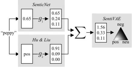
[image:1.595.306.526.262.375.2]Sentiment lexica provide an easy way to automat-ically label texts with polarity values, and are also frequently transformed into features for supervised models, including neural networks (Palogiannidi et al., 2016; Ma et al., 2018). Indeed, given their utility, a veritable cottage industry has emerged focusing on the design of sentiment lexica. In prac-tice, using any single lexicon, unless specifically and carefully designed for the particular domain of interest, has several downsides. For example, any lexicon will typically have low coverage compared to the language’s entire vocabulary, and may have misspecified labels for the domain. In many cases, it may therefore be desirable to combine multiple sentiment lexica into a single representation. Indeed, some research on unifying
Figure 1: A depiction of the “encoder” portion of Sen-tiVAE. The wordpeppyhas polarity values of 0.65 and
posin the SenticNet and Hu-Liu lexica, respectively. These values are “encoded” into two three-dimensional vectors, which are then summed and added to(1,1,1) (not shown) to form the parameters of a Dirichlet over the latent representation of the word’s polarity value.
such lexica has emerged (Emerson and Declerck, 2014; Altrabsheh et al., 2017), borrowing ideas from crowdsourcing (Raykar et al., 2010; Hovy et al., 2013). However, this is a non-trivial task, because lexica can use binary, categorical, or continuous scales to quantify polarity—in addition to different interpretations for each—and thus cannot easily be combined. In Fig. 1, we show an example of the same word labeled using different lexica to illustrate the nature of the challenge.
lex-Lexicon Source N Dom
SentiWordNet WordNet 14107 [−1,1]2
MPQA Newswire 4397 {0,1} SenticNet — 100000 [−1,1] Hu-Liu Product reviews 6790 {0,1}
GI — 4206 {0,1}
VADER Social media 7489 {0, . . . ,8}10
Table 1: Descriptive statistics for the sentiment lexica. N: vocabulary size. Dom: Domain of polarity values.
ica, we are able to derive a common latent represen-tation of the words’ polarities. The resulting model is spiritually related to a multi-view learning ap-proach (Sun, 2013), where each view corresponds to a different lexicon. Experimentally, we use SentiVAE to combine six commonly used English-language sentiment lexica with disparate scales.
We evaluate the resulting representation via a text classification task involving nine English-language sentiment analysis datasets. For each dataset, we transform each text into an average polarity value using either our representation, one of the six commonly used sentiment lexica, or a straightforward combination thereof. We then train a classifier to predict the overall sentiment of each text from its average polarity value. We find that our representation outperforms the individual lex-ica, as well as the straightforward combination for some datasets. Our representation is particularly efficacious for datasets from domains that are not well-supported by standard sentiment lexica.1
The existing research that is most closely re-lated to our work is SentiMerge (Emerson and De-clerck, 2014), a Bayesian approach for aligning sentiment lexica with different continuous scales. SentiMerge consists of two steps: (i) aligning the lexica via rescaling, and (ii) combining the rescaled lexica using a Gaussian distribution. The authors perform token-level evaluation using a single senti-ment analysis dataset where each token is labeled with its contextually dependent sentiment. Because SentiMerge can only combine lexica with continu-ous scales, we do not include it in our evaluation.
2 Sentiment Lexica and Scales
We use the following commonly used English-language sentiment lexica: SentiWordNet (Bac-cianella et al., 2010), MPQA (Wilson et al., 2005), SenticNet 5 (Cambria et al., 2014), Hu-Liu (Hu and
1Our representation and code are available athttps://
github.com/ahoho/SentiVAE.
Liu, 2004), GI (Stone et al., 1962), and VADER (Hutto and Gilbert, 2014). Descriptive statistics for each lexicon are shown in Tab. 1. Each word in SentiWordNet is labeled with two real values, each in the interval[0,1], corresponding to the strength of positive and negative sentiment (e.g., the label (0 0)is neutral, while the label(1 0)is maximally positive). Each word in VADER is labeled by ten different human evaluators, with each evaluator pro-viding a polarity value on a nine-point scale (where the midpoint is neutral), yielding a 10-dimensional label. MPQA, Hu-Liu, and GI all use binary scales. Lastly, each word in SenticNet is labeled with a real value in the interval[−1,1], where 0 is neutral.
3 SentiVAE
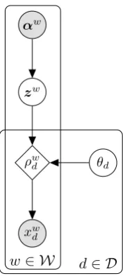
We first describe a figurative generative process for a single sentiment lexicond∈ D, whereDis a set of sentiment lexica. Imagine there is a true (latent) polarity value zw associated with each word w
in the lexicon’s vocabulary. When the lexicon’s creator labels that word according to their chosen scale (e.g., thumbs-up or thumbs-down, a real value in the interval[0,1]), they deterministically transform this true value to their chosen scale via a function f(·;θd).2 Sometimes, noise is introduced during this labeling process, corrupting the label as it leaves the ethereal realm and producing the (observed) polarity labelxwd. They then add this potentially noisy label to the lexicon. Given a lexicon of observed polarity labels, the latent polarity values can be inferred using a VAE. The original VAE posits a generative model of ob-served dataX and latent variablesZ:P(X,Z) =
P(X | Z)P(Z). Inference ofZthen proceeds by
approximating the (intractable) posteriorP(Z | X) with a Gaussian distribution, factorized over the in-dividual latent variables. A parameterized encoder function compressesX intoZ, while a parameter-ized decoder function reconstructsX fromZ.
SentiVAE extends the original VAE model to combine multiple lexica with disparate scales, pro-ducing a common latent representation of the polar-ity value for each word in the combined vocabulary.
Generative process. Given a set of sentiment lexicaD with a combined vocabulary W, Senti-VAE posits a common latent representationzw of the polarity value for each wordw∈ W, wherezw
is a three-dimensional categorical distribution over
αw
zw
ρw
d θd
xwd
w∈ W d∈ D
Figure 2: Generative model for SentiVAE.
the sentimentspositive,negative, andneutral. The generative process starts by drawing each latent polarity valuezwfrom a three-dimensional Dirichlet prior, parameterized byαw = (1,1,1):
zw∼Dir(αw). (1)
If the word is uncontroversial,3 we spur this prior somewhat using the number of lexica in which the word appears c(w). Specifically, we add c(w) to the parameter for the sentiment associated with that word in the lexica, e.g.,
αSUPERB= (1 +c(SUPERB),1,1). This has the
ef-fect of regularizing the inferred latent polarity value toward the desired distribution over sentiments.
Having generatedzw, the process proceeds by “decoding” zw into each lexicon’s chosen scale. First, for each lexicon d ∈ D, zw is determinis-tically transformed via neural network f(·;θd) with a single 32-dimensional hidden layer, parameterized by lexicon-specific weightsθd:
ρwd =f(zw;θd). (2)
The transformed valueρwd is then used to generate the (observed) polarity labelxwd for that lexicon:
xwd ∼Pd(xwd |ρwd). (3)
The dimensionality ofρwd and the emission distribu-tionPdare lexicon-specific. For SentiWordNet,Pd
3
We say that a word is uncontroversial if there is strong agreement across the sentiment lexica in which it appears. Even without this spurring, the inferred latent representation typically separates into the three sentiment classes, but perfor-mance on our text classification task is somewhat diminished.
Dataset Source N Classes
IMDB Movies 25000 2
Yelp Product reviews 100000 5 / 3
SemEval Twitter 7668 3
MultiDom Product reviews 6500 2
ACL Scientific reviews 248 5 / 3
[image:3.595.137.226.59.259.2]ICLR Scientific reviews 2166 10 / 3
Table 2: Descriptive statistics for the training portions of the sentiment analysis datasets.N: number of texts.
is a two-dimensional Gaussian with meanρwd and a diagonal covariance matrix equal to0.01I; for VADER,Pdconsists of ten nine-dimensional cate-gorical distributions, collectively parameterized by
ρwd; for MPQA, Hu-Liu, and GI,Pdis a Bernoulli distribution, parameterized by ρwd; and for Sen-ticNet,Pdis a univariate Gaussian with mean and variance each an element in a two-dimensionalρwd.
Inference. Inference involves forming the pos-terior distribution over the latent polarity values
Z given the observed polarity labelsX. Because computing the normalizing constant P(X) is in-tractable, we instead approximate the posterior with a family of distributionsQλ(Z), indexed by
variational parametersλ. Specifically, we use
Qλ(Z) = Y
w∈W
Qβw(zw) = Y
w∈W
Dir(βw). (4)
To construct βw, we first define a neural net-workg(·;φd), with a single 32-dimensional hid-den layer, which “encodes” xwd into a three-dimensional vector. The output of this neural net-work is then transformed via a softmax as follows:
ωwd =softmax g(xwd;φd)
(5)
βw = 1 +X d∈D
ωdw. (6)
The intuition behind βw can be understood by appealing to the “pseudocount” interpretation of Dirichlet parameters. Each lexicon contributes ex-actly one pseudocount, divided among positive,
negative, andneutral, to what would otherwise be a symmetric, uniform Dirichlet distribution. As a consequence of this construction, words that ap-pear in more lexica will have more concentrated Dirichlets. Intuitively, this property is appealing.
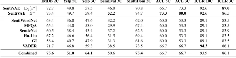
IMDB 2C Yelp 5C Yelp 3C SemEval 3C MultiDom 2C ACL 5C ACL 3C ICLR 10C ICLR 3C
SentiVAE EQ[zw] 72.7 49.8 57.5 46.0 70.8 66.7 73.3 92.6 87.0 SentiVAE βw 73.4 49.7 59.4 52.2 74.7 73.3 80.0 92.6 86.5
SentiWordNet 63.4 36.0 47.6 32.2 62.0 60.0 53.3 89.1 83.5 MPQA 65.4 44.0 53.0 29.9 67.4 60.0 53.3 89.1 83.5 SenticNet 60.5 38.4 43.4 37.2 62.3 60.0 53.3 89.1 83.9 Hu-Liu 67.2 46.6 56.4 31.5 69.4 60.0 53.3 89.1 83.5 GI 58.4 40.7 47.9 31.3 61.6 60.0 53.3 89.1 83.5 VADER 71.7 46.8 59.3 38.5 73.5 66.7 66.7 94.3 86.1
[image:4.595.71.525.68.181.2]Combined 75.6 51.0 64.1 50.6 75.4 66.7 66.7 93.9 86.1
Table 3: Classification accuracies for our representation, six lexica, and a straightforward combination thereof.
et al., 2013) using Adam (Kingma and Ba, 2015) in the Pyro framework (Bingham et al., 2018). The standard reparameterization trick used in the origi-nal VAE does not apply to models with Dirichlet-distributed latent variables, so we use the general-ized reparameterization trick of Ruiz et al. (2016).
4 Experiments and Results
To evaluate our approach, we first use SentiVAE to combine the six lexica described in §2. For each wordwin the combined vocabulary, we ob-tain an estimate of zw by taking the mean of
Qβw(zw) = Dir(βw)—i.e., by normalizing βw.
We compare this representation to using βw di-rectly, becauseβwcontains information about Sen-tiVAE’s certainty about the word’s latent polar-ity value. We evaluate our common latent rep-resentation via a text classification task involving nine English-language sentiment analysis datasets: IMDB (Maas et al., 2011), Yelp (Zhang et al., 2015), SemEval 2017 Task 4 (SemEval, Rosen-thal et al. (2017)), multi-domain sentiment analysis (MultiDom, Blitzer et al. (2007)), and PeerRead (Kang et al., 2018) with splits ACL 2017 and ICLR 2017 (Kang et al., 2018). Each dataset consists of multiple texts (e.g., tweets, articles), each labeled with an overall sentiment (e.g.,positive). Descrip-tive statistics for each dataset are shown in Tab. 2. For the datasets with more than three sentiment la-bels, we consider two versions—the original and a version with only three (bucketed) sentiment labels.
For each dataset, we transform each text into an average polarity value using either our represen-tation, one of the six lexica,4or a straightforward combination thereof, where the polarity value for
4
We bucket the upper four and lower four points of VADER’s nine-point scale, to yield a three-point scale. With-out this bucketing, our representation With-outperforms VADER on four of the nine datasets. We do not bucket VADER when using it in SentiVAE or in the straightforward combination.
each word in the (combined) vocabulary is a 16-dimensional vector that consists of a concatenation of polarity values. (Unlike SentiVAE, this concate-nation does not yield a single sentiment lexicon that retains scale coherence, while achieving maxi-mal coverage over words.) Specifically, we replace each token with its corresponding polarity value, and then average the these values (Go et al., 2009;
¨
Ozdemir and Bergler, 2015; Kiritchenko et al., 2014). We then use the training portion of the dataset to learn a logistic regression classifier to predict the overall sentiment of each text from its average polarity value. Finally, we use the testing portion to compute the accuracy of the classifier.
Results. The results in Tab. 3 show that our rep-resentation usingβw outperforms the individual lexica for all but one dataset, and that our repre-sentation using the mean ofQβw(zw)outperforms
them for six datasets. This is likely because Senti-VAE has a richer representation of sentiment than any individual lexicon, and it has greater coverage over words (see Tab. 4). The results in Tab. 5 sup-port the former reason: even when we limit the words in our representation to match those in an individual lexicon, our representation still outper-forms the individual lexicon. Unsurprisingly, our representation especially outperforms lexica with unidimensional scales. We also find that our rep-resentation outperforms the straightforward com-bination for datasets from domains that are not well supported by the individual lexica (see Tabs. 1 and 2 for lexicon and dataset sources, respectively). By combining lexica from different domains, our representation captures a general notion of senti-ment that is not tailored to any specific domain.
5 Conclusion
IMDB SemEval Multi ICLR
SentiVAE 70 64 81 71
SentiWordNet 15 14 24 16
MPQA 10 7 18 9
SenticNet 40 39 53 45
Hu-Liu 7 5 13 5
GI 8 7 15 6
[image:5.595.84.280.208.322.2]VADER 7 6 13 5
Table 4: Coverage over words (percentage) by lexicon for the training portions of four of the nine datasets.
IMDB 2C SemEval 3C
SV Lex SV Lex
SentiVAE 74.7 – 72.4 –
SentiWordNet 70.6 63.4 67.4 55.1
MPQA 73.5 66.6 62.6 51.8
SenticNet 74.4 60.9 72.1 59.5
Hu-Liu 73.6 68.4 59.1 51.1
GI 71.4 59.3 63.8 54.0
VADER 73.6 73.1 60.9 58.7
Table 5: Classification accuracies for a 10% validation portion of two of the datasets. The first row, labeled SentiVAE, contains the classification accuracy for our representation usingβw. Subsequent (lexicon-specific) rows compare our representation (SV), restricted to the vocabulary of that lexicon, to the lexicon itself (Lex).
latent representation, and realized this model with a novel multi-view variational autoencoder, called SentiVAE. We then used SentiVAE to combine six commonly used English-language sentiment lex-ica with binary, categorlex-ical, and continuous scales. Via a downstream text classification task involving nine English-language sentiment analysis datasets, we found that our representation outperforms the individual lexica, as well as a straightforward com-bination thereof. We also found that our represen-tation is particularly efficacious for datasets from domains that are not well-supported by standard sentiment lexica. Finally, we note that our approach is more general than SentiMerge (Emerson and De-clerck, 2014). While SentiMerge can only combine sentiment lexica with continuous scales, SentiVAE is designed to combine lexica with disparate scales.
Acknowledgements
We would like to thank to Adam Forbes for the de-sign of Fig. 1. We further acknowledge the support of the NVIDIA Corporation with the donation of the Titan Xp GPU used to conduct this research.
References
Nabeela Altrabsheh, Mazen El-Masri, and Hanady Mansour. 2017. Combining Sentiment Lexicons of Arabic Terms. InAMCIS. Association for Informa-tion Systems.
Stefano Baccianella, Andrea Esuli, and Fabrizio Sebas-tiani. 2010. SentiWordNet 3.0: An Enhanced Lex-ical Resource for Sentiment Analysis and Opinion Mining. 10(2010):2200–2204.
Eli Bingham, Jonathan P. Chen, Martin Jankowiak, Fritz Obermeyer, Neeraj Pradhan, Theofanis Kar-aletsos, Rohit Singh, Paul A. Szerlip, Paul Horsfall, and Noah D. Goodman. 2018. Pyro: Deep Universal Probabilistic Programming. CoRR, abs/1810.09538.
David M. Blei, Alp Kucukelbir, and Jon D. McAuliffe. 2017. Variational inference: A review for statisti-cians. Journal of the American Statistical Associa-tion, 112:859–877.
John Blitzer, Mark Dredze, and Fernando Pereira. 2007. Biographies, Bollywood, Boom-boxes and Blenders: Domain Adaptation for Sentiment Classification. In
Proceedings of the 45th Annual Meeting of the As-sociation of Computational Linguistics, pages 440– 447, Prague, Czech Republic. Association for Com-putational Linguistics.
Erik Cambria, Daniel Olsher, and Dheeraj Rajagopal. 2014. SenticNet 3: A Common and Common-sense Knowledge Base for Cognition-driven Sen-timent Analysis. In Proceedings of the Twenty-Eighth AAAI Conference on Artificial Intelligence, AAAI’14, pages 1515–1521. AAAI Press.
Guy Emerson and Thierry Declerck. 2014. Sen-tiMerge: Combining Sentiment Lexicons in a Bayesian Framework. In Proceedings of Work-shop on Lexical and Grammatical Resources for Language Processing, pages 30–38. Association for Computational Linguistics and Dublin City Univer-sity.
Alec Go, Richa Bhayani, and Lei Huang. 2009. Twitter Sentiment Classification using Distant Supervision.
Processing, pages 1–6.
Matthew D. Hoffman, David M. Blei, Chong Wang, and John William Paisley. 2013. Stochastic varia-tional inference. Journal of Machine Learning Re-search, 14(1):1303–1347.
Dirk Hovy, Taylor Berg-Kirkpatrick, Ashish Vaswani, and Eduard H. Hovy. 2013. Learning Whom to Trust with MACE. InProceedings of the 2013 Con-ference of the North American Chapter of the Asso-ciation for Computational Linguistics: Human Lan-guage Technologies, pages 1120–1130. Association for Computational Linguistics.
ACM SIGKDD International Conference on Knowl-edge Discovery and Data Mining, pages 168–177. ACM.
C. J. Hutto and Eric Gilbert. 2014. VADER: A Parsi-monious Rule-Based Model for Sentiment Analysis of Social Media Text. InEighth International Con-ference on Weblogs and Social Media (ICWSM-14).
Dongyeop Kang, Waleed Ammar, Bhavana Dalvi, Madeleine van Zuylen, Sebastian Kohlmeier, Ed-uard H. Hovy, and Roy Schwartz. 2018. A Dataset of Peer Reviews (PeerRead): Collection, Insights and NLP Applications. InProceedings of the 2018 Conference of the North American Chapter of the Association for Computational Linguistics: Human Language Technologies, Volume 1 (Long Papers), pages 1647–1661. Association for Computational Linguistics.
Diederik P. Kingma and Jimmy Ba. 2015. Adam: A method for stochastic optimization. InInternational Conference on Learning Representations (ICLR).
Diederik P. Kingma and Max Welling. 2014. Auto-Encoding Variational Bayes. InProceedings of the Second International Conference on Learning Rep-resentations (ICLR).
Svetlana Kiritchenko, Xiaodan Zhu, and Saif M. Mo-hammad. 2014. Sentiment Analysis of Short Infor-mal Texts. Journal of Machine Learning Research, 50:723–762.
Yukun Ma, Haiyun Peng, and Erik Cambria. 2018. Tar-geted Aspect-Based Sentiment Analysis via Embed-ding Commonsense Knowledge into an Attentive LSTM. InAAAI, pages 5876–5883. AAAI Press.
Andrew L. Maas, Raymond E. Daly, Peter T. Pham, Dan Huang, Andrew Y. Ng, and Christopher Potts. 2011. Learning Word Vectors for Sentiment Analy-sis. InProceedings of the 49th Annual Meeting of the Association for Computational Linguistics: Hu-man Language Technologies, pages 142–150, Port-land, Oregon, USA. Association for Computational Linguistics.
Canberk ¨Ozdemir and Sabine Bergler. 2015. A Com-parative Study of Different Sentiment Lexica for Sentiment Analysis of Tweets. InProceedings of the International Conference Recent Advances in Natu-ral Language Processing, pages 488–496. INCOMA Ltd. Shoumen, BULGARIA.
Elisavet Palogiannidi, Athanasia Kolovou, Fenia Christopoulou, Filippos Kokkinos, Elias Iosif, Niko-laos Malandrakis, Haris Papageorgiou, Shrikanth Narayanan, and Alexandros Potamianos. 2016. Tweester at SemEval-2016 Task 4: Sentiment Anal-ysis in Twitter Using Semantic-Affective Model Adaptation. In Proceedings of the 10th Interna-tional Workshop on Semantic Evaluation (SemEval-2016), pages 155–163. The Association for Com-puter Linguistics.
Vikas C. Raykar, Shipeng Yu, Linda H. Zhao, Ger-ardo Hermosillo Valadez, Charles Florin, Luca Bo-goni, and Linda Moy. 2010. Learning From Crowds.
Journal of Machine Learning Research, 11:1297– 1322.
Sara Rosenthal, Noura Farra, and Preslav Nakov. 2017. SemEval-2017 Task 4: Sentiment Analysis in Twit-ter. In Proceedings of the 11th International Workshop on Semantic Evaluation (SemEval-2017), pages 502–518, Vancouver, Canada. Association for Computational Linguistics.
Francisco R. Ruiz, Michalis K. Titsias, and David M. Blei. 2016. The Generalized Reparameterization Gradient. InAdvances in Neural Information Pro-cessing Systems, pages 460–468.
Philip J. Stone, Robert F. Bales, J. Zvi Namenwirth, and Daniel M. Ogilvie. 1962. The general inquirer: A computer system for content analysis and retrieval based on the sentence as a unit of information. Be-havioral Science, 7(4):484–498.
Shiliang Sun. 2013. A Survey on Multi-view Learning.
Neural Computing and Applications, 23(7-8):2031– 2038.
Theresa Wilson, Janyce Wiebe, and Paul Hoffmann. 2005. Recognizing Contextual Polarity in Phrase-Level Sentiment Analysis. In Proceedings of Hu-man Language Technology Conference and Confer-ence on Empirical Methods in Natural Language Processing, pages 347–354, Vancouver, British Columbia, Canada. Association for Computational Linguistics.