Cognitive agents and machine learning by example : representation with conceptual graphs

warwick.ac.uk/lib-publications

Gkiokas, Alexandros and Cristea, Alexandra I. (2018) Cognitive agents and machine learning

by example : representation with conceptual graphs. Computational Intelligence

. doi:10.1111/coin.12167 Permanent WRAP URL:

http://wrap.warwick.ac.uk/98279

Copyright and reuse:

The Warwick Research Archive Portal (WRAP) makes this work by researchers of the University of Warwick available open access under the following conditions. Copyright © and all moral rights to the version of the paper presented here belong to the individual author(s) and/or other copyright owners. To the extent reasonable and practicable the material made available in WRAP has been checked for eligibility before being made available.

Copies of full items can be used for personal research or study, educational, or not-for profit purposes without prior permission or charge. Provided that the authors, title and full bibliographic details are credited, a hyperlink and/or URL is given for the original metadata page and the content is not changed in any way.

Publisher’s statement:

"This is the peer reviewed version of the following Gkiokas, Alexandros and Cristea,

Alexandra I. (2018) Cognitive agents and machine learning by example : representation with conceptual graphs. Computational Intelligence . doi:10.1111/coin.12167 (In Press)

which has been published in final form https://doi.org/10.1111/coin.12167 . This article may be used for non-commercial purposes in accordance with Wiley Terms and Conditions for Self-Archiving."

A note on versions:

The version presented here may differ from the published version or, version of record, if you wish to cite this item you are advised to consult the publisher’s version. Please see the ‘permanent WRAP URL’ above for details on accessing the published version and note that access may require a subscription.

Cognitive Agents and Machine Learning by Example: Representation with

Conceptual Graphs

ALEXANDROSGKIOKAS, ALEXANDRAI. CRISTEA

Computer Science Department, University of Warwick,CV3 7AL, Coventry, United Kingdom

AsMachine LearningandArtificial Intelligenceprogress, more complex tasks can be addressed, quite often by cascading or combining existing models and technologies, known as the bottom-up design. Some of those tasks are addressed by agents, which attempt to simulate or emulate higher cognitive abilities that cover a broad range of functions; hence those agents are namedcognitive agents. We formulate, implement and evaluate such a cognitive agent, which combineslearning by examplewith machine learning. The mechanisms, algorithms and theories to be merged when training a cognitive agent to read and learn how to represent knowledge, have not, to the best of our knowledge, been defined by the current state-of-the-art research. The task oflearning to represent knowledge is known assemantic parsing, and we demonstrate that it is an ability that may be attained by cognitive agents using machine learning, and the knowledge acquired can be represented by usingconceptual graphs. By doing so, we create a cognitive agent that simulates properties of ’learning by example’, whilst performing semantic parsing with good accuracy. Due to the unique and unconventional design of this agent, we first present the model, and then gauge its performance, showcasing its strengths and weaknesses.

Key words:Learning by Example, Machine Learning, Cognitive Agents, Semantic Parsing, Conceptual Graphs.

i

1. INTRODUCTION

The task of reading a sentence and representing it using an ontology model is

called semantic parsing (Popescu et al., 2003) a process which uses semantics in

order to translate text to a knowledge representation structure. This process is

nor-mally algorithmic, based upon heuristics, statistics or other rules (Tang and Mooney,

2001; Shi and Mihalcea, 2005; Wong and Mooney, 2006), or in more recent

re-search, relies on Deep learning (Andor et al., 2016; Weiss et al., 2015; Zhang and

McDonald, 2012) .Such a process might simulate the mechanism through which we

acquire knowledge and information (Vlachos and Clark, 2014; Vlachos, 2012). A

cognitive agent simulates the functions which enable humans to perform semantic

parsing, rather than implementing semantic parsing as a machine-oriented

mecha-nism. Therefore it is sound to presume that a cognitive agent capable of performing

such a function with relative ease, would be one step closer to becoming able to

autonomously learn indefinitely.

Hence, a major target for an intelligent cognitive agent is the ability to learn

how to represent knowledge fromextracted information, and in this use-case, from

raw text (Craven et al., 1999). The criteria, as set by (Lawniczak and Di Stefano,

2010) are perception, reasoning with and judgement of information or knowledge,

as well as the most important achievement, the ability tolearn new knowledgefrom

information.

This ability may be allowing forsimulative biomimicry, if built upon biologically

the input text and symbols onto a knowledge representation (KR) structure, which

correctly describes all currently knownsemiotic informationabout that input. Doing

so can involve the usage of semantics, statistics, annotated meta-data related to

grammatical properties, ontologies, and many other characteristics and attributes.

Hereinafter, we describe and analyse an agent which combines different AI

mod-els, in order to achieve the goal of learning how to correctly represent information

onto conceptual graphs. The goal is to attain semantic parsing, by teaching the agent

how to perform such a task. The algorithms involved in performing semantic parsing

are not based on any prior knowledge. Instead, the agent first learns by examples and

observation, then self-analyses the learnt material, and is finally tested on unknown

material.

The work described hereinafter addresses some of Bach’sSynthetic Intelligence

requirements (Bach, 2009), e.g., perception, experience, cognition and emotion (via

reinforcement) and Haikonen’s (Haikonen, 2012, 2009) cognitive intelligence topics

such as meaning and representation and their relation to information, association and

memory, and a rudimentary form of reasoning (discussed in Section 2.1).

The unique novelty in our approach is that we avoid previously used rigid

ap-proaches, rule-based models, heuristics and templates, (Tang and Mooney, 2001; Shi

and Mihalcea, 2005; Pradhan et al., 2004; Zhong et al., 2011; Poon and Domingos,

2009) which albeit performing well, are severely limited to the domains, languages,

or even to the input size. On the contrary, we describe, evaluate and provide evidence

that a cognitive agent based upon machine learning models, can provide robust

and adaptive semantic parsing, by learning by example, regardless of the domain.

learning with artificial neural sub-controllers, data-mining, semantics and statistics.

We have designed it in a manner which enables it to learn from examples the user

provides, and self-organises and controls its internal experience and knowledge, in

order to enable accurate and continuous learning, whilst being able to be retrained

and updated. This agent starts in a blank/tabula rasastate. When trained by a user, it

is able to recreate the semantic parsing process, thus performing the task in the same

manner as the trainer.

Moreover, previous research in semantic parsing and other related fields rely

on feature vectors, and not on the actual symbols (tokens,words) (Clarke, 2015;

Grefenstette et al., 2014; Pradhan et al., 2004). This is due to the computational

power required, memory space needed to process individual tokens and the increase

in execution time, when working with raw information. Thus the norm for the past

decade or so, has been to work on text using feature vectors and vector spaces,

rather than directly on the actual text, with only a handful exceptions where a direct

representations was used (Liang and Potts, 2015; Wong and Mooney, 2006).

Current more recent research in semantic parsing, using Deep Learning and other

types of AI models, still rely on feature vectors (Grefenstette et al., 2014; Clarke,

2015). These researches vary different models, architectures, designs and algorithms

on the aforementioned vectors. On the other hand, non-vector related research uses

statistical approaches (Wong and Mooney, 2006) and relies on word-alignment and

other well-formatted rules. Reinforcement learning andimitation-basedapproaches

(Vlachos and Clark, 2014; Andreas et al., 2013; Vlachos, 2012) use machine learning

as an action-selection mechanism dealing with features, rather than as a

Recentstate-of-the-art made significant breakthrough in accuracy, attributed to

deep learning. The most recent breakthrough is from Google (Andor et al., 2016;

Weiss et al., 2015; Zhang and McDonald, 2012) and the use ofTensorFlow(Abadi

et al., 2016) library as used by SyntaxNet (Petrov, 2016). Google relied mostly

on POS tagging (the Parsey McParseface POS tagger) rather than Semantics, yet

achieved the best F1 scores to date (F1 results range from 94.44% on news data,

95.40% on question-answers and 90.17% on web data).

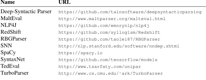
Other state-of-the-artis the research and platform by thespaCy(Honnibal and

Johnson, 2015) start-up in Germany. Current software, tools and platforms

consid-ered state-of-the-art are shown in Table 1 (State of the Art NLU Software Tools);

for a full list and analysis Choi et al (Choi et al., 2015) have gauged performance,

accuracy, speed, etc., yet some platforms have been renamed, and some appear to be

un-maintained or deprecated since then.

[Table 1 about here.]

Our main contribution is thus that we provide a radical new approach to

seman-tic parsing, where the agent learns a whole temporal-spatial sequence on how to

construct knowledge representations of the input.

In the above context, the agent treats the construction of the CG as a

tempo-ral process, e.g., a Shift-Reduce operation (Sagae, 2009; Sagae and Lavie, 2006;

Shieber, 1983) whilst the spatial aspect of the processing focuses on operations

on the graph being constructed. Such an approach, to the best of our knowledge,

Markovian staterepresented by the graph itself. As such, a symbolic KR (the CG) is

being learnt by a learning mechanism.

Prior research in using conceptual graphs for semantic parsing, compared to

Meaning Representation Languages (MRL) or other KR schemes, is sparse and

inconclusive (Zhong et al., 2011; Montes-y G´omez et al., 2002). Moreover, the latter

research relies solely on heuristics, or semi-supervised learning. Instead, we support

the notion that heuristics should be replaced by machine learning, to eliminate the

necessity of prior knowledge of the domain and hard-coded rules or templates.

How-ever, the notion of using CG to extract knowledge, as well as reason with it

(Kamsu-Foguem and Chapurlat, 2006) isn’t new. Manipulation of knowledge graphs in

real-life applications has been researched in the past (Ruiz et al., 2014; Kamsu-Foguem

et al., 2013), and as such it stands to reason that usage of CG in cognitive agents

could enable better human-agent interaction, especially forknowledge transference.

The Machine-Learning based cognitive agent is further compared with the most

representative and successful heuristic and semi-supervised state of the art solutions,

to clarify and illustrate its strengths and weaknesses.

2. LEARNING MODEL

2.1. Theoretical Model

Figure 1 (Agent Schema) demonstrates a high level of the components of the

agent1,and how they interact with each-other (Gkiokas, 2016).

[Figure 1 about here.]

The agent uses KR to store knowledge acquired from raw information. The KR

model that does the actual representation of knowledge is the conceptual graph (CG)

model of Sowa (1999). Conceptual graphs are finite connected bipartite graphs with

entities partitioned as either concepts or relations (Chein and Mugnier, 2008).

Con-ceptual graphs were chosen because they are simplistic and minimal models without

an excess of meta-data. Other advantages are the simplification of the representation

and relations through labelled edges, their expressiveness, which is similar to natural

language, and their accuracy and highly structural information (Rasli et al., 2014;

Zhong et al., 2011). Furthermore, other researchers (Croitoru et al., 2007) state

that conceptual graphs are intuitive and semantically sound means of knowledge

representation. Most importantly, conceptual graphs have been demonstrated to offer

a computationally tractable and sound way of representing text and natural language

(Montes-y G´omez et al., 2002). Within the cognitive agent’s memory, we describe a

conceptual graphGt = (Vt, Et)at a moment in timet, as shown in (1), with nodes

V = (Ct, Rt)being either concepts or relations, and using edges (E) between node

classes, to form a bipartite graph. This model is implemented as an adjacency list

for graphGtwhich also describes a statest.

Gt= (Ct, Rt, Et). (1)

We have used an adjacency list, as it has O(|V| + |E|) storage complexity,

O(1)vertex and edge addition, andO(|V|)query complexity (Cormen et al., 2001).

Using an adjacency matrix would offer faster queries, but it has larger memory

stores thousands of conceptual graphs in its memory, we chose theadjacency list, as

it has the fastest addition and most conservative memory requirements. Indeed, these

operations occur very frequently when learning graphs, since the agent manipulates

an empty graph into a populated one, by adding nodes and edges. We do not remove

vertexes or edges, and thus anincidence listwould not be beneficial, as neither would

be anincidence matrix(Coxeter, 1973).

In order to learn the construction of a conceptual graph, the cognitive agent uses

reinforcement learning (Sutton and Barto, 1998) a neural-temporal learning

mech-anism, which we have implemented using the Q-Learning algorithm (Sutton and

Barto, 1998, equation 6.6) - one of the most frequently used algorithms due to its

per-formance. We chose Reinforcement Learning because it is a biologically plausible

mathematical representation of behaviouristic Psychology learning, by simulating

how agents learn by associating a cumulative reward with their actions (Watkins,

1989; Sutton, 1984; Galef Jr, 1988). Furthermore, using Reinforcement Learning

allows us to represent and handle symbolic representations (e.g., the graphs) directly

on a ML algorithm in aMarkoviansense (Howard, 1970; Bellman, 1957).

At the highest and most abstract level, the agent observes examples provided by

the user, decomposes them, learns by their decomposition, and then becomes able

to (a) recreate them, or (b) use them to approximate how to performhighly similar

tasks. Figure 2 (Agent Observation and Recreation) demonstrates that high level

approach in simplistic terms.

[Figure 2 about here.]

policy value of taking action at in state st. The reward R is obtained only at the

terminal state and is back-propagated to the previous states. The constant α is the

learning rate, and constant γ is the discount factor of the next policy’s value; both

constantsαandγhave a range between 0 and 1.

[Figure 3 about here.]

The rewarding cycle, as shown in Figure 3 (Agent Reward), is not continuous

and takes place once when the agent has finished performing the task. In this case

theenvironment is in fact the Conceptual Graph being manipulated, and the reward

is associated to a specific input and output.

A low learning rate tends to ignore updates, whereas a high learning rate

con-siders the most recent updates. Similarly, a low discount rate makes the algorithm

opportunistic with respect to the most recent rewards, whereas a conservative-long

term approach requires a high discount value (Even-Dar and Mansour, 2004). After

trial and error and through empirical testing we decided to useα= 0.7andγ = 0.3,

the reason being that due to the way the cognitive agent learns, by being presented

examples only once, we prefer fast learning of the most recent reward. Because the

same episode will not be re-iterated multiple times (as it is the case withprobabilistic

Q-learning, or when re-experiencing same or similar episodes), faster learning

im-plies less time spent on training, a notion similarly described inOne-Shot Imitation

learning(Duan et al., 2017) for Robotics.

Q(st, at)=Q(st, at) +α[R(t)+γ·max

a Q(st+1, a)−Q(st, at)]. (2)

learn-ing can be used directly on symbolic information and the KR byproduct, as the

state st denotes a KR structure at a moment in time: the conceptual graph Gt of

that instance. Using theMarkov Decision Process(MDP) employed by Q-Learning

to describe the process (named an episode) of creating a conceptual graph, is also

the basis upon which the agent learns how to perform the projection operation of

information onto KR. Thus, the agent processes the actual text, structures and labels,

rather than the features of the input. This approach affectswhat the agent is learning;

not features or meta-data from vectorised information or vector space models, but the

actual representation, as it is being created from the input information.

The agent aims to accumulate background knowledge (conceptual graphs) and

experience (policies - episodes) when trained, in order to maximise its accuracy and

overall performance. It is employingclassification methods(see Sections 2.3.2, 2.3.3

and 2.3.4), which are combined as sub-controllers of the main reinforcement learning

algorithm. The forefathers of reinforcement learning (Sutton and Barto, 1998)

men-tioned that an ensemble of learning and other function approximation methods are

necessary, in order to be able to reuse policies. The states and actions, the building

blocks of reinforcement learning, are learnt via Q policies. By learning the correct

policies about the projection of text onto conceptual graphs, the approximation of

states and actions enables reusability of previous experiences (episodic and

non-episodic), when presented with new input (see Section 6).

In reinforcement learning an episode~et_{is a sequence ofstatess}

tjoined together

by their actions at, where t is a time-step that describes a moment in time, thus

creating a MDP. Each episode is made up of a variable number of states and has a

~

et:{(st=1, at=1),(st=2, at=2),· · · ,(st=n, at=n)}. (3)

Each state describes the transition and projection of symbolic information(text)

towards a conceptual graph. The state is described here in a Markovian manner, by

a set oftokenisedwordsTt, and the current conceptual graphGt, for the time-stept

(see definition 4).

st: (

Tt :{w1, w2,· · · , wn}

Gt:{Ct, Rt, Et}

)

. (4)

As the agent projects information (e.g., tokens, words, symbols) asnodesonto

the graph Gt, these tokens are removed from the next state’s st+1 token set Tt+1.

Thus, the token set is a stack from which words are removed as the episode

pro-gresses, and the graph is populated with nodes, it is in fact ashift-reduce(Shieber,

1983) operation. When the token setTtbecomes empty, the agent has to connect the

nodes of graphGt, by using edges. Once the agent is certain that no more edges must

be created, it terminates the episode, by producing a terminal state. Theconceptual

graphof that terminal state is the final product of the projection:the representation

of the information given as input.

An action at can be the decision to convert a token to aconcept orrelation, as

conceptual graphs are bipartite graphs. The decision to take actionatis what creates

new states, the transitional link from st to st+1 in the episode ~et. In addition to

creating nodes, an action can also be the decision to createedgesbetween concepts

[Figure 4 about here.]

The Figure 4 shows howShift-Reduceis used in the MDP to populate the graph

with nodes, and then how it is used to create edges between the nodes. This process is

deterministic(and therefore we use the deterministic version of Q-Learning) because

the agent can determine the result of its action at any given moment. Furthermore,

the MDP has no hidden states or partial hidden states, albeit the semiotics of a state

are not assumed to be all known.

The actions are created by the agent, and can be generated byrandom, semantic,

probabilistic algorithms, or classified via neural networks,as those are the models

and algorithms most often used in recent related research (Choi et al., 2015; Andor

et al., 2016; Weiss et al., 2015; Clarke, 2015; Zhang and McDonald, 2012;

Grefen-stette et al., 2014; Vlachos and Clark, 2014; Andreas et al., 2013; Vlachos, 2012;

Zhong et al., 2011; Poon and Domingos, 2009; Shi and Mihalcea, 2005; Pradhan

et al., 2004; Tang and Mooney, 2001). Each of the described approaches, models

and algorithms is described below, and evaluated in Section 6.

In the literature (Sutton and Barto, 1998) actions are created and then evaluated

via a fitness function. As actions directly affect the next state and therefore the

produced outcome, a good action generation mechanism is crucial in a cognitive

agent and it is highly beneficial to avoid searching; instead it is preferred to

approxi-mate new actions based on previous ones. We examine all individual action creation

mechanisms in Sections 2.3.1, 2.3.2, 2.3.3 and 2.3.4.

Cascading various algorithms was done empirically, as well as by relying on

overall accuracy. The methods tested (and described hereinafter) were based on

previous research using Heuristics, Probabilities, Semantics and Machine Learning.

During training, the graph G and the associated input sentence are given as a

paradigm or example, which the agent observes and analyses, in order to infer the

episode and learn from it. Once the agent has recreated an episode for that graph, it

presumes that the example is correct, and thus reinforces it with a positive reward,

hence reinforcing the episode that created that graph.

As part of the training process (see section 3.1), a decomposition algorithm

disassembles an existing graph G into an episode~et_{, and its corresponding states}

and actions. The graph is part of the training data, and has already been created

by a human user as the example from which to learn. The actions are inferred by

observing the graph changes between states: word to node conversion and graph

edge creation. The decomposition algorithm is a naive heuristic, but is required in

order to infer the associated states and actions; its output is a pair of st, at, part of

the episode used to train the agent. During testing,the agent may be presented with

known, unknown, or partially known input. When the agent is givenknown input, it

stays on-Policy and simply outputs what Q-Learning dictates (see formula 2). For

partially known input, the classification mechanisms are responsible for creating

new actions by reusing previous episodes. The classification mechanisms depend on

reusing previous Q(st, at) policies, either directly or indirectly. In the event where

unknown input is given, the agent has to explore and thus discover new policies, by

2.2. Input pre-processing

When the agent is given a sentence as input, that input is tokenised, using

stan-dard white-space tokenizing, and certain English particles are removed (e.g.: ”a”,

”an”, ”the”), as well as common symbols such as commas, question-marks, and

full-stops. This is done in order to offer a ’cleaner’ input to the agent, as it is

rec-ommended by (Jurafsky and Martin, 2000). Furthermore, apart-of-speechprocessor

obtains the tags for each tokenised word in the sentence (Tsuruoka et al., 2011). In

addition to the aforementioned pre-processing, aVector Space Model(Turney et al.,

2010) is built as a sparse matrix, and indexes all input sentences, so thatattributional

semanticscan be used, to find input sentences similar to the ones stored in the agent’s

memory. However, no rules or templates are applied, the input is not pre-annotated

with semantics, ontologies, entities, or in any other way.

2.3. Action Decision

The importance of correct actions needstobe emphasised: incorrect actions lead

to incorrect states, which eventually create incorrect conceptual graphs. The

accu-racy of the terminal state and its corresponding conceptual graph is what dictates the

overall performance of the agent.The agent learns how to create the actual

represen-tation, by learning to perform the correct sequence ofactionsfor each corresponding

state.Thus it does notclassify or categorisea conceptual graph; it creates correct or

incorrect terminalgraphs. It is those graphs we used to reward the agent, and also

to infer how accurateit is, in comparison to the expected graph output. We discuss

accuracy metrics in Section 6.1, using Sørensen coefficient (12) and Jaccard index

The cognitive agent has a variety of action creation mechanisms at its disposal,

and some are used in a cascading or preferential manner (meaning, one algorithm

takes precedence over another), whereas other action creation mechanisms (i.e.,

neu-ral networks) are used as standalone. We have implemented and evaluated various

action-selection mechanisms from previous research, ranging from Relational

Se-mantics (Fellbaum, 1998) to a statistical approach, a naive Bayesian and others. The

action-decision mechanisms are used only when testing the agent; during training,

the actions are inferred from the observedexamples.

An explanation of each algorithm follows. We use a variety, not only to test

which works better, but to compare to other research, which relies on similar

algo-rithms.

2.3.1. Random Action. A random action is based upon a uniform random

distri-bution, and utilises the Mersenne twister (Matsumoto and Nishimura, 1998)

pseudo-random generator (PRNG). The Mersenne twister is the most widely used PRNG and

it offers a fast and secure implementation for random integers. In the action-decision

deployment scenario, it randomly decides if a word is aconceptor arelation, and if

two nodes should be connected by anedge.

2.3.2. Semantic Action. A semantic action uses WordNet (Fellbaum, 1998) to

obtain hypernyms, hyponyms and synonyms as graphs, which it then traverses, in

order to detect if two queried words aresemanticallyconnected, and what their

se-mantic similarity is. We chose WordNet, as it is the only dictionary-based framework

widely used for discovering semantic relations; it has also been evaluated and tested

sentences. Other languages would require both a WordNet database to be used, and

a POS tagger capable of processing that language.

Quantifying the semantic similarity, denoted byδ[n,n0_], is done using the formula

(5), as below.

δ[n,n0_]=w_s i

k=layers(si)

X

k=0

t[n,n0_]

1 +β d[n,n0_]

. (5)

The nodesnandn’representwords,tokensorlabels, which become the queries

to WordNet. When a graph (representing a hyponym, hypernym or synonym tree)

is processed, the distance travelled is stored int[n,n0_], whereas the traversal direction

d[n,n0_](forwards or backwards) is alleviated by the constantβ(empirically set to 0.1).

The min-max normalised sense weightwsi(set by WordNet) biases towards the most

frequent senses, which always appear first, according to the way they are sorted in

WordNet dictionaries, from the most frequent to the least frequent. By using this

semantic similarity, the agent may decide to recreate a known actionat, which was

operating on noden, because it is very similar to noden’, for which a policyQ(st, at)

already exists.

2.3.3. Probabilistic Action. The cognitive agent, after being trained with

exam-ples, analyses its episodic memory and all policies acquired. By data mining its

own episodic memory statistics, it acquires frequencies of events and observations,

such as the rate of token to node conversion, or edges existing between nodes.

By obtaining statistics from observing the frequency of events, the agent is able to

calculate empirical binomial probabilities. Probabilities are calculated by querying

the probability of an edge existing for a node tuple, denoted as P(∃(e[n,n0_])) the

equation 6). The opposite also holds true: 6 ∃(e[n,n0_]) denotes the fact that such an

edgehas not been observed to existbut could have been created due to the presence

ofnandn0. Thus, formula (6) describes the empirical probability of an edge existing,

with respect to the total observations for that edge and thenodes that it can connect.

P(∃(e[n,n0_])) =

P

∃(e[n,n0_])

P _∃

(e[n,n0_])+P 6 ∃(e_[n,n0_])

. (6)

When computing edge probabilities, we may use either the token value (the label)

or the POS Tag of the token (its syntactic attribute). A combinatorial probability may

also be used, in the event that both edge probabilities are known. All probabilities

recorded have arangebetween 0 and 1, and are recorded foredgesandnodes. Token

to node probability (equation 7) is recorded for both tokens and POS tags, i.e.,

measuring how frequently a specific tag (or token/word) is classified as a concept

or relation.

P(Concept) = #of Events(t=Concept)

#of Observations(t) . (7)

In the above formula (7), the number of events where a token twas being

clas-sified as a concept, are divided by the number of total observations made about t.

Exactly the same rule applies for calculating relation probabilities. In this formula,t

can be either a token, or a token’s part-of-speech tag. Token distance is a probability

value based on the observation of distance events (e.g., how far were two tokens

2.3.4. Neural Actions. Twomulti-layer feed forward artificial neural networks

(ANN) are created and trained after thedata-miningphase. One network is trained

using POS Tags and token distance, the other is trained using POS tags, tokens and

token distance. The reason for doing this is that P(token) is not always available,

whereas P(P OS) is always available (as computed by formula (7)). After being

trained, and after performing data-mining on the action/policy observations, the

probability values can be calculated for every edge observed. We do not train the

ANN on token-to-node action selection, because probabilistic actions perform a

highly accurate node recognition (as further discussed in section 6).

The probability values for edges (see equation (6)) and the scaled and normalised

token distance between the tokens within the input sentence, are the actual ANN

in-put data. The architecture of the networks has been optimised by using thecascading

algorithm(Nissen, 2003), and was further optimised, by using early stopping(Yao

et al., 2007) through cross validation of the mean-square error. Optimisation was

necessary as the problem of over-fitting became an issue, mostly due to the usage of

noise in large training sets. Empirical hyper-parameter optimisation, albeit a topic

on its own accord, directly affects the agent’s output and as such we examined

how different parameters and approaches could be used to yield the best possible

neural-based action selection. Furthermore, we used training data sub-sampling and

random shuffling, in order to ensure correct representational efficiency. The selection

of the neural network parameters (hidden neurons) is a big challenge, with over 20

years of research in the area (Sheela and Deepa, 2013; Hagan et al., 1996), and no

definite answer. Here, we used an anecdotal formula (Stackexchange, 2015) which

neurons (see eq. 8), where Nh is the number of hidden neurons needed, Ni is the

number of input neurons, and No is the number of output neurons, whilst Ns is

the number of training samples. The constant alphais normally said to be a value

between 5 and 10, but through trial and error we established that a value of 12 was

more suitable for our intents and purposes, as it avoided overfitting.

Nh =

Ns

alpha∗(Ni+No)

. (8)

Neural action controllers can be said to act as filters or classifiers, which decide

if an edge should be created or not. They act as sub-controllers, processing the

extracted probabilities from the data-mining done by the agent, when iterating its

episodic memory.

2.4. State Classification

Similar states are classified using only the original input sentence. This is

per-formed via the use of a Vector Space Model (Turney et al., 2010), which has the

ability to find very similar input in the agent’s memory. This model allows the agent

to assume that highly similar input may have similar output graphs. Classification

was done by training an ANN to take into account the similarity between states,

using themin-maxnormalised VSM similarity from equation (9) as the input value

which affects the action-decision mechanism. In the equation,mis the vector space,

andndenotes the vectorised input sentence, where pn, tm are the matrix coefficient

Am,n =              

p1t1 p1t2 p1t3 . . . p1tm

p2t1 p2t2 p2t3 . . . p2tm

p3t1 p3t2 p3t3 . . . p3tm

..

. ... ... . .. ...

pnt1 pnt2 pnt3 . . . pntm               . (9)

3. AGENT ALGORITHMS

3.1. Training

During training, the agent learns how to project input onto conceptual graphs.

An inference algorithm breaks down conceptual graphs to their nodes and edges,

and then infers node actions, by observing which words were converted to what

node types; it then finds the edges which connected those nodes, thus inferring

edge actions. The algorithm (1) is inspired byprogramming by example(Lieberman,

2001); in essence, it is neuro-dynamic programming (Bertsekas and Tsitsiklis, 1995),

which creates an MDP, in the form of an episode~et.

The training is done in batches, and thus results in many episodes and their

corresponding conceptual graphs, populating the agent’s memory. Each batch size

depends upon the actual data-set used to train the agent (see Section 4). Every time

the agent is trained, it is done without it having any a-priori knowledge about the

domain or the data-set, with the only exception being the POS tag annotation by

laPOS (Tsuruoka et al., 2011) (see Sections 2.3.3 and 2.3.4).

Every episode acquired during training is positively rewarded, as the agent

ad-Algorithm 1Batch Training Loop

tuples =load(trainset)

for tuple[graph, text]∈tuples do

episode=array[st, at] for word∈tuple.text do

at =f indN odeInGraph(word, paradigm.graph)

episode.add(st, at)

gt=st

addN ode(gt, at)

st+1 =gt

Remove(st+1, word)

for edge∈tuple.graph do

at =f indEdgeInGraph(gt) if st¬terminal then

episode.add(st, at)

gt =st

addEdge(gt, at)

st+1 =gt

U pdateP olicies(episode,1.0)

vantages (Nehaniv and Dautenhahn, 2007) but also some pitfalls. Admittedly some

limitations do exist: since this agent learns from the user, should the user provide

erroneous examples, the agent will simply learn them. Ambiguity and contradictory

paradigms also create dissonance within the agent’s memory, and in some cases

can severely hinder the agent’s performance. A phenomenon, which, as known, is

inherent from the imitative ability of animals and humans. Dissonance is filtered via

statistics, but this approach also affects special cases such as patterns where general

probabilities do not apply.

Furthermore, because the focus is Natural Language (NL), a common issue often

encountered is that of ambiguity (Gorrell, 2006), which is related to both the

syntac-tic and semansyntac-tic properties of NL. That ambiguity can (and often does) createnoise

memory. Because the agent does not attribute importance to the information source,

or the frequency that a specific sample may appear, e.g., all samples are given equal

policy weights in the memory, hence an exception to a rule, i.e., an outlier might

influence the overall agent memory. A scoring or bias system, could potentially

address this issue; we’ve used classical probabilities in order to filter out the outliers,

but admittedly more sophisticated approaches such as feature selection and detection

may increase accuracy. Perhaps, most interesting of all,judgementorscoringof the

training source (e.g., person or resource) could provide a more robust agent, but the

complexity of such a system would increase, and would have to be unsupervised

since the agent would have to be capable of adjusting policies in its memory.

3.2. Data-Mining

The agentdata-mines(Algorithm 2) its own episodic memory after being trained,

in order to deduce and calculate probability values, as described in section 2.3.3, and

the agent updates look-up tables for those probability values. Themodus operandiis

straightforward: the agent will create all possible permutations of tokens into nodes,

and then observe which ones actually exist in a given episode, as actions in the known

Q(st, at)policies. Similarly, it creates edge permutations for existing nodes within

an episode’s graph, and then observes which ones did exist. This creates amapping

of the possibleaction search space for a given episode input, which the agent then

uses to update the probability values for tokens, POS Tags, and token distances.

The actual size and values recorded depend on the data-set used to train the agent.

Hence, larger data-sets create larger and potentially more accurate probability

6.5), which is then used either by theProbability Actionmechanism (section 2.3.3),

or the artificial neural network action mechanism (section 2.3.4).

Algorithm 2Data-Mining edges

for episode∈memory do

sterminal =episode.end()

gt=sterminal

for relation∈gt do for concept∈gt do

action=Edge(relation, concept)

if action∈episode then

Record(P R(relation, concept, T rue)

else

Record(P R(relation, concept, F alse)

for concept∈gt do for relation∈gt do

action=Edge(relation, concept)

if action∈episode then

Record(P R(relation, concept, T rue)

else

Record(P R(relation, concept, F alse)

3.3. Testing

Testing is done after the agent has been trained, and it has data-mined its episodic

memory space. Thus, testing assumes that the agent is trained on some subset that

is representational of the information given when being tested, and that some kind

of action-decision mechanism exists (e.g., neural, random, semantic, etc). If the

pro-duced conceptual graph of the terminal state isequivalent(identical or isomorphic)

to the one associated with the tuple’s input, then the agent self-rewards its decisions

positively, else the episode is regarded as erroneous and is therefore rewarded

Algorithm 3Testing loop

policies=load(M emory) examples=load(P aradigms)

for test∈examples do

graph=test.graph input=test.text st=new(input) if st 6∈policiesthen

episode=new(empty)

while at =Decide(st) do

st =inf er(input, at)

episode.add(st, at)

st+1 =calculateN ext(st, at)

st =st+1 terminal =st

if terminal.graph≡graph then

U pdateP olicies(episode,1.0)

elseIfterminal.graph6≡graph U pdateP olicies(episode,−1.0)

else

while ∃ Q(st, at)

∧st¬T erminal do

Online(Q(st, at))

4. CONCEPTUAL GRAPH DATA-SETS

The domain data used in this paper is taken from health related news articles,

scientific discoveriesandlifestyle articles,and has been published on GitHub2_{. The}

reason for our selection is that, whilst allowing for reasonable complexity

(em-pirically observed during construction and annotation of the data-set), in terms of

unknown words and more complex graph structures, such articles tend at the same

time to be quite straightforward and factual, containing state-of-fact or discovery,

thereby being less ambiguous in their description. Using factual or statement

ori-ented sentences isn’t a requirement, but evidence suggests that this type of text input

is more structured and less ambiguous, for example Google’s Syntaxnet (Andor

et al., 2016; Weiss et al., 2015) which provided the best to dateF1scores of 94.44%

on news data and 95.40% on question-answer data, but only 90.17% on Web data.

This type of performance is consistent across various studies (Andor et al., 2016;

Weiss et al., 2015; Zhang et al., 2014; Martins et al., 2013). Our intention therefore

was to test with varying degrees of sentence complexity (small, medium and large

sentences) without dealing with Web-related data.

The articles were collected from a variety of on-line resources (RSS feeds) from

BBC, Sky News, USA Today, Science Daily and Knox News. Both the title and actual

content of the RSS feeds were used to create the data-set. The titles were used

to create smaller graphs, whereas the article contents were used to expand on the

same topic and create larger and more complex graphs. The content is also further

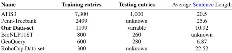
partitioned into many graphs, by using full-stops as the delimiter. In total, the

data-set has 1199 entries, and each entry is a tuple: a text sentence and its corresponding

conceptual graph. The dataset size was limited by the fact that it had to be generated

manually. However, the total data-set size was deemed fit for these experiments, as

other datasets in use were of similar or smaller size (see Table 2 - Commonly used

Data-sets).

[Table 2 about here.]

The data-set has a variety of entries: some are short sentences (and thereby small

graphs) and some are long and complex. All subsets were created randomlyin the

same fashion, by shuffling tuple entries and then randomly choosing the ones with a

set and a testing set. The larger subsets also contain entries from the smaller subsets,

but the agent is never tested with different sets in the same experiment, to avoid

encountering these overlapping entries. The average length of a sentence increases

from set to set, from 5 words per input up to 30 words per input. Figure 5 (Graph

Example) shows an example of a simple CG.

[Figure 5 about here.]

The most commonly used data-sets for testing similar tasks in the literature (e.g.,

semantic parsing) are displayed in Table 2. As can be seen, only two sets are larger

than our set. However, these sets cannot be directly compared, for reasons as follows.

ATIS3 (Hemphill et al., 1990), which is significantly larger, having evolved over

the course of decades, offers transcribed utterances dissimilar to scientific news

and feeds. It aims to provide a question-answer scenario, that is not applicable to

our cognitive agent scenario. Similarly, the Penn-Treebank 3 (Marcus et al., 1993)

containsWall Street Journal stories, with syntactic annotation. They are not

appro-priate for our agent, as they contain abbreviations, US-English, stock names and

symbols, etc. TheRoboCupdata-set (Chen and Mooney, 2008; David L. Chen, 2010)

organises the data inMeaning Representation Language (MRL)logical form tuples,

containing phrases used in theRoboCupsoccer championship, quite dissimilar from

our domain. The BioNLP11ST (by the BioNL Shared Task organisation) is a

data-set focusing on co-reference, entity relations and gene renaming. The last and largest

difference is that all aforementioned data-sets use either MRL, logical formulae, or

other similar KR structures. With the exception of (Campbell and Musen, 1992) who

conceptual graph data-set currently exists. Still, even with these differences, the

comparison to the data-sets in Table 2 serves to demonstrate that our data-set size is

comparable with other datasets in current use,however, the average word length per

sentence is smaller than what is often used. The reason for that is mostly related to

practicality; the CG dataset was created for the purpose of testing this agent, and as

such the effect of large and complex sentences is already known and established from

previous research (Choi et al., 2015). What we are mostly interesting is not gauging

how well the agent compares to other research, but if it performs its intended tasks,

which are however comparable to other research. As seen later in Section 6, the agent

does stay on par with other related NL research.

[Figure 6 about here.]

However it is important to note that our data-set partitioning is biased towards

smaller average sentences, with the overall average size being 8 words per sentence,

as shown in Figure 6 (Dataset Characteristics). The variation observed in accuracy

(later discussed in Section 6), is mostly attributed to that wide range of changing

sub-set datasets being tested.

We hypothesise that whilst the complexity of the tuple entries is not entirely

dependent upon the input word count, it is a good indicator, as the larger the input

in words/tokens, the larger the search space becomes for the agent, and hence the

solution to the input is more difficult. Other simple complexity measures include

the node to edge ratio, the average path length of a graph, all indicators of the

such as betweenness, radius, closeness, clusterization (Wright, 1977; Barooah and

Hespanha, 2007) as those were outside ofthescope of our work.

The average VSM (Vector Space Model) similarity is yet another metric, which

indicates how attributionally similaris the topmost similar episode in the memory

of the agent, to the one being produced (Turney et al., 2010). We average the

top-most VSM similarity for all inputs, in order to establish if the agent has already

processed some input which is similar. The implication is that subsets with higher

VSM similarity would be easier for the agent to evaluate, as its acquired policies

during training wouldmost likely be applicableto the given input when testing.

5. EXPERIMENTAL METHODOLOGY

Experimentation is done by first training the cognitive agent, using one of the

training subsets, and then testing it with the corresponding testing subset, following

the principles of Simulated Experiments (Winsberg, 2003). This approach ensures

that tuple entries in the training set will never be present in the testing set. Each

experiment was done using a random subset of the dataset, and the memory of the

agent is deleted across different experiments,so that we can average the accuracy and

account for randomness and noise. The experimental methodology remains constant

for all experiments, and a variety of meta-data is logged, in order to infer accuracy,

performance, and monitor algorithm usage. Moreover, instead of training the agent

on the same training-set, we use random samples of the training set, which are

mutu-ally exclusive. Ensuring consistent performance is done not only by randomising the

and its respective testing set (Cavazzuti, 2012). This approach known asRandomized

Complete Block Design(Higgins, 2003; Winer et al., 1971) organises in small blocks

of experiments similar input-length sub-sets randomly picked, and proceeds to repeat

each one ten times, and then averages their performance.

5.1. Training

The training methodology is as follows: (i) delete the agent’s previous memory,

(ii) instruct the agent to load the training set, (iii) train the agent, (iv) perform

data-mining, (v) save all memory (policies, probabilities, etc.) on the disk. The training

phase is entirely separated from the testing phase. The agent is trained incrementally,

by observing and analysing one paradigm at a time.

5.2. Testing

The testing methodology is as follows: (i) load its memory (from training), (ii) do

testing phase, (iii) log every produced graph, (iv) log VSM similarity, (v) log graph

node-edge ratio, word input length, and other metrics, (v) log amount of random,

probabilistic, semantic and neural actions. At the end of each testing experiment, a

script is run which extracts certain metrics obtained during execution.

Those metrics are averaged to evaluate: (i) average node similarity, (ii) average

edge similarity, (iii) average graph similarity, (iv) average input length. The total

number of experiments used 12 blocks of random subsets executing each one 10

6. RESULTS

6.1. Overall Agent Performance

Due to the nature of conceptual graphs using sets of relations, concepts and

edges, it is justifiable to treat graph similarity as a problem of set matching. As

our implementation of conceptual graphs usesadjacency lists(see equation (1)) we

have identified and used two different methods to calculate graph similarity: the

Similarity Coefficient (Rijsbergen, 1979) also known as Sørensen index or Dice’s

coefficient (see equation (10)) and the Jaccard Index (Real and Vargas, 1996) or

Jaccard coefficient (see equation (11)), which compute the similarity between two

setsAandB.

S(A∼B) = 2|A∩B |

|A|+|B |. (10)

J(A∼B) = |A∩B |

|A|+|B | − |A∩B |. (11)

Both similarity coefficientsserve the purpose of measuring how similar the agent’s

output, e.g., a produced graph G is, to the ideal or target output graph G0. The

difference between Sørensen and Jaccard coefficients is that Sørensen ignores the

amount of different items in the set, whereas Jaccard penalises the set difference,

thus resulting in a smaller similarity value if the two sets contain many different

items.

When establishing the agent accuracy, a norm widely used in binary

classifica-tion is theF1score (Brodersen et al., 2010). However, this score is not directly

appli-cable to our work, due to the fact that the notions ofprecisionandrecall(Brodersen

generation of CG as output. The Jaccard coefficient is a more strict measure which

ideally would be used, however the Dice-Sørensen coefficient has the same form

as the F1 score (Intan et al., 2015, p. 158) and therefore functions as the primary

accuracy quantifier. It is also important to note that similarity is respective to the first

graph in Dice-Sørensen: the formula quantifies only how similar Gis to G0 and its

parameters are non-anadrome.

We use the term average graph similarity, referring to the similarity coefficient

of thetargetoutput graph and theactualgraph for both (10) and (11), a value scaled

and normalised between zero and one. Using a similarity coefficient withconcepts,

relations and edges from the graphs G and G0 provides the basis upon which we

have computed the agent’s performance.

For Sørensen coefficient we weighted nodesVG = (C, R)of both classes equally

to edges, in order to avoid biasing the final value favourably towards nodes. Equal

importance is thus attributed to all entities of the graph, and hence to all actions of

the agent, due to the fact that agent actionsatconstruct the final graph.

S(G∼G0) = 1

2 · S(CG ∼CG0) +S(RG ∼RG0)

+S(EG ∼EG0)

2 . (12)

The Jaccard coefficient is used differently: each set C, R and E uses its size as a

ratio, thus the final value not only penalises different items in sets, but if a set is

larger, then it weighs more in the final score.

J(G∼G0) = |CG | ·J(CG, CG0)+ |RG| ·J(RG, RG0)+|EG | ·J(EG, EG0)

|CG |+|RG|+|EG |

.

(13)

Boolean terms and as a percentile. The opposite also holds true, two graphs which

have no common nodes or edges will have agraph similarityof 0.

Figure 7 shows how Sørensen and Jaccard accuracy for all experiments change,

with respect to different data-sets. As the average sentence length (input) decreases,

the agent becomes much more accurate. As expected, the subset with the smallest

input was able to reproduce most accurately the output, whilst the subsets with

a higher count of words and thus complexity, had significantly lower accuracy.

Sørensen/F1core and Jaccard have a very narrow distribution curve for the average

accuracy of all experiment subsets. However, we report the average accuracy for the

largest data-set (the one containing the most complex and large input) in Table 3.

[Figure 7 about here.]

The first observation is that the overall accuracy and graph similarity are not

linearly related; in fact quite the contrary appears to take place, where small edge

similarity fluctuations have a disproportionate effect on the graphaccuracy. Due to

the fact that node accuracy remains constantly high and above 95% for all

exper-iments, we can only attribute this drop to the decrease in edge accuracy; it is

in-fact the only metric which seems to decrease, as input complexity increases, hence

influencing the graph similarity. The implication of this effect is important, as it

signifies that edge accuracy is what hinders the overall agent accuracy, albeit a small

but noticable decline in node accuracy could also affect edge accuracy.

In order to further examine the effect of node and edge accuracy, we logged the

percentage of node and edge actions (out of the total actions) for every experiment.

were 44.39%. This ratio could further augment the negative effect incorrect edges

have on correct output: for example 88.65% of edge similarity could in fact play

a more significant role in the output, when more edge actions than node actions

are performed. Thus the Jaccard index we implemented (shown in equation (13))

weighing edges, appears to have a sharper decline, very similar to that of the edge

similarity decline, whilst node similarity remains highly accurate.

6.2. Complexity and Accuracy

As Figure 7(Agent accuracy)shows, the agent was able toconsistently provide

anF1 Score of 92.78% for the entire data-set (e.g., all sentence input sizes).

Taking into account the fact that the data-sets in the right side of the plot in Figure

(6)have increasing complexity(see Section 4),this indicates that the cognitive agent

manages to stay on par with previous related research (Zhong et al., 2011), and

demonstrates the ability to construct complex conceptual graphs.

In Figure 8 we have used the logged data from our experiments: Sørensen

co-efficient, Jaccard index, graph node-edge ratio, average graph path length and edge

search space. We performed Principal Component Analysis (Wold et al., 1987) (PCA)

on: (a) the similarity coefficients(Sørensen and Jaccard) asAccuracy (PCA), and (b)

the word input length and edge search space as Input Complexity (PCA), thereby

representing the overall similarity with respect to edge search space and word input

changes. In order to plot multiple dimensional data, we have projected the most

significant Eigenvectors on a single (lower) dimension: one dimension for Accuracy

(PCA), and one dimension for graph Input complexity (PCA). Thus the

search space, and the ”accuracy” metric is the compressed row of the PCA from

theJaccard and Sørensendata columns. This was done for all experimental results,

as seen in Figure 8, whilst identifying how complexity affects accuracy and agent

performance. In Figure 8, the graph path-size (how ”deep” a graph is), the graph

node-edge ratio |_|V_E|_|, and the synthetic (PCA) ”complexity” metric are shown, as a

Q-normalised 3D surface. The right plot in Figure 8 shows the 4th dimension as a

colour heatmap, the ”accuracy”, and how graph attributes and complexity relate to

graph accuracy.

[Figure 8 about here.]

The first observation (see Figure 8) is that complexity is directly related to agent

accuracy. Another, less obvious factor that seems to influence agent accuracy is a

small node-edgeratio |_|V_E|_|, which implies that sparsely connected graphs are harder

to construct, compared to dense or fully connected graphs. An untested hypothesis

which would explain this phenomenon, is that sparse graphs tend to branch in a

variety of different ways, thus making sub-pattern recognition harder. Observing

Figure 8 clearly demonstrates that graphs which are ”column-like”, i.e., have few

branches, are a lot easier to construct. The last important observation is that albeit

graph path-size increases as complexity increases (which is to be expected), it does

not have a detrimental effect on graph construction.

6.3. Data-mining Results

Using Data-Miningto perform probability value extraction via graph

a complete mappingof the action search space, but it is not a random sub-sampling

either: it is a mapping of all possible actions related to a specific input. We did

not use boot-strapping, random sub-sampling or other techniques to acquire data for

training the ANN, because smaller training sets were empirically found togeneralise

too much, and offer little advantages over simple probabilistic algorithms. Thus, we

arrived to the conclusion that, although a permutation mapping of a large action

space was time-consuming, it warrantedmore representationalprobability samples,

due to the fact that data-mining provided considerably larger frequency/probability

samples. Furthermore, the conclusion was further supported by the fact that ANNs

trained with larger training data outperformed every other algorithm, as discussed in

Section 6.4.

[Figure 9 about here.]

We also examined the distribution of the data-mined data after training. Figure 9

depicts the data-mined probability histograms. The first histogramP r(edge[T oken])

shows the probability (see equation (6)) of an edge connecting two tokens, based

on their label, e.g., their token value. It has an unusual distribution, with a mean

x= 0.27and standard distributionσ= 0.37, evident by the high frequency samples

at the extremes. This is not a sampling error but indicates that most observed events

were either correct, or incorrect, due to edges created using token probabilities.

Because most samples have near-zero probability, the agent learnt which edges to

avoid based on tokens values alone. The middle histogram P r(Edge[P OST ag])is

the probability (see equation (6)) of an edge based on Part-of-Speech tags. It has

probability’s distribution implies that POS tags offer a rather general approach to

calculating edges, and more often than not, do not offer a high degree of certainty

for an action at. The bottom histogram is not a probability, but the normalised and

scaled (0 to 1) values of token distance within a sentence, which have been observed

to become connected by an edge. We data-mined it because it aids the agent by

correctly inferring if an edge, which would otherwise be highly probable to exist,

should be in fact filtered out, due to an extreme distance of the two tokens inside the

sentence. It has a mean ofx= 0.04and a standard deviation ofσ= 0.55.

[Figure 10 about here.]

In Figure 10 we used the data shown as histograms previously in Figure 9, and

plotted it in three dimensions. The top leftpoint-cloudis the representation in space

of all 30,960 samples taken from low-value and high value actions. The visual

demonstration showcases the correlation of the samples to theentire action search

space, not taking into account the affinely extended real number system and its

implications, but assuming discrete integral values. The uppermost left plot in Figure

10 shows that in the entire search space, only a small amount has been sampled,

when using graph permutation actions from the episodic memory of the agent. The

topmost right plot in Figure 10 is a three-dimensional grid surface, which connects

the points, and thus generalises the data, by using theQ-normfunction for all

data-points. The bottom left plot contains the three dimensional Convex Hull (Chazelle,

1993) of the points, superimposed on the cloud. The bottom right plot contains the

same Convex Hull, superimposed on the normalised data grid surface. All plots in

Figure 9), the edge probability based on POS tags (second histogram in Figure 9)

for the Y axis, and the normalised token distance (third histogram in Figure 9) as

theZ axis. One evident conclusion from Figure 10 is that the samples are not large,

when taking into to the actual search space, yet they provide enough representational

value to allow the agent to become sufficient. Considering that the search space may

become larger, as more tokens (words) are introduced, the constraining factors are

the fixed set of POS Tags, and the fact that token distances are scaled and normalised.

The second conclusion related to this form of data-mining via action

permuta-tions, is that the data appears to be non-linearly separable, due to the fact that the

convex hull visually appears to intersect closely clustered data-points (Toussaint,

1983); we did not however use any applicable methodology (Elizondo, 2006) to

verify this observation. This observation justifies the usage of a multi-layered ANN,

as it is beneficial when compared to other algorithms, since it allows to efficiently

map and classify data collected from data-mining post-training ashigh value actions.

6.4. Algorithm Comparison

We compared the various action algorithms employed within the cognitive agent.

The baseline performance measured as a ”random walk” was the random action

controller (Section 2.3.1). All other action selection controllers were tested either

isolated (e.g., the only action selection mechanism active) or fused together, in a

cascading mode, starting from probabilistic, to semantic and random, or semantic

to probabilistic and random. The neural action controller was tested in combination

the best cascade of the remaining controllers was probabilistic, to semantic and

random.

Cascading Semantic with probabilistic, and probabilistic with semantic showed

that preferential execution of probabilistic before falling back to Semantic was

sig-nificantly better as average graph similarity. Probabilistic execution was optimised,

by combining probabilities and by using them in a preferential manner, where

to-ken probability was chosen over POS tag probability. An explanation for this

phe-nomenon is the debate of generality over granularity; probabilities based on POS tags

are presumed to be generalising action decisions, whereas token-based probabilities

offer a much more granular approach, but are not always available, since the agent

may be given unknown tokens or unseen tokens. Semantic action selection, when run

semi-isolated (using only a random selector as a fall-back), showed a marginally

bet-ter than random accuracy. As aforementioned, VSM similarity only shows thatsome

episodes are similar up to a certain degree, and because the Semantics algorithm

relies on finding VSM-similar episodes, it most often was unusable. Furthermore,

smaller data-sets have a low average VSM similarity, thus feature vectoring was not

of much use to the agent. Other data-sets had higher average VSM similarity, but

also a higher graph complexity.

A comparison of the probabilistic and neural controllers provides some insight as

to why neural-based approaches may in fact be more suitable than statistical-based

approaches in the field of cognitive agents. The neural controller is trained using

probability values and scaled distance values, but it develops the ability to filter,

classify and differentiate good from bad actions, whereas the probabilistic controller

controller uses both probability values and scaled/normalised arithmetic values, it

outperforms the empirical probability controller. We have optimised and tried

nu-merous experiments with probability-based controllers, including a naive Bayesian

filter; however, we found that a large multilayer feed-forward neural network always

provided better results.

6.5. Artificial Neural Networks as Action Controllers

Due to the nature of neural networks, and more specifically their random weight

initialisation, variable performance was observed. Shuffling training data, and using

Batch Training, combined with the optimisation techniques mentioned in Section

(2.3.4), we proceeded to optimise ANNs, due to strong indications that they would

outperform other algorithms. Initially, the ANNs were not consistent throughout

experiments, and were trained on-the-fly, right after data-mining. This induced a

very generalised classification of actions, which proved inefficient and inaccurate.

Eventually we accumulated data during multiple data-mining passes and gained a

larger training sample for the ANN.

What Figure 11 demonstrates, is the progression from a small and generalising

ANN, which used a small training sample, towards a fine tuned (and large) ANN,

which used a highly representational training sample. The X axes represent the

POS Tag probability values, the Z axes represent the token/node distance within

a sentence (normalised and scaled to -1 and 1) and the Y axes show the token

edge probabilities (formula (6)). That is the same data acquired during data-mining

(Section 3.2, 6.3, Figure 10), with the action value superimposed as a colour. The

green are correctactions, and redincorrectactions. The early ANN was small (less

than 10 neurons) and used a small training sample, but as the agent kept data-mining,

larger training samples were acquired. The steepness of the angle in the ANN shows

the token distance sampling, whereas the spikes and crevices show particular areas

of extreme token distance samples. The final ANN was quite large (300 neurons)

and with 3 layers, of which one is a hidden layer.

[Figure 11 about here.]

We proceeded to train multiple neural networks, and used the best optimised one

for all experiments, regardless of the data-set. ThebestANNs for our purpose were

empirically selected, not only via the hyper-parametrisation techniques

aforemen-tioned, but though cross-validation by experimentation using various data-sets as

input. We avoided over-training by using early stopping (Yao et al., 2007), whilst

retaining good generalisation. Due to the nature of optimising hyper-parameters and

ANN architecture, it is plausible that the reported accuracy may further be improved.

The optimal neural network was selected out of a group of many networks,

because it provided consistently the best results across all data-sets with which it

was tested. Continuous updating of the probabilities look-up table enabled us to

create a very large training sample set for the ANNs. Furthermore, by iterating the

episodic memory of the agent, and trying all sorts of permutations as operations on

graphs, and then filtering the known high Q-value actions, we were able to create

an accurate map of high value actions and associate them with input and episodes.

(Y axis) and only a small fraction of high probability POS Tag edges (X axis) are

associated withhigh valueQ(st, at)policies.

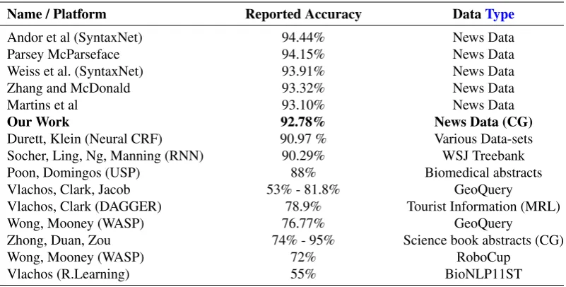
6.6. Comparison to State-of-the-Art

In order to determine how well the cognitive agent performed, in comparison to

some of the most recent and related research, we have used the reported accuracy by

their respective authors, as shown in Table (3).

[Table 3 about here.]

Most of the results provided in Table (3) are obtained by using annotated or

formatted data. This needs to be emphasised, as we did not annotate data (with the

exception of the POS-tagging), nor did we use utterances, question-answer

scenar-ios, bi-grams or tri-grams. Our data was partitioned, with input text lengthranging

from 4 to 30 words, as resulted from the harvested data sets. Choi et al mention that

most parsers have a UAS accuracy of 93.49 to 95.5 for sentences under 10 terms,

which declines to 81.66 and 86.61 for sentences larger than 50 terms. Examining

Table (3), (Zhong et al., 2011) used a manual template model, and reported 85%

to 88% accuracy on concept entities, and 74% to 95% accuracy on relations

(pos-sesive, function, broader, style, content). Our average entity accuracy was higher

(96.90%). Moreover, Zhong et al. do not mention conceptual graph accuracy, nor do

they provide information about their datasets, or the edge accuracy. In comparison,

our cognitive agent combines unsupervised learning (reinforcement learning via

examples), with semi-supervised learning (for the ANN), and self-supervised