Identifying efficient solutions via simulation : myopic multi objective budget allocation for the bi objective case

https://doi.org/10.1007/s00291-019-00561-0

R E G U L A R A R T I C L E

Identifying efficient solutions via simulation: myopic

multi-objective budget allocation for the bi-objective case

Juergen Branke1 _{·Wen Zhang}1

Received: 10 July 2018 / Accepted: 1 August 2019 © The Author(s) 2019

Abstract

Simulation optimisation offers great opportunities in the design and optimisation of complex systems. In the presence of multiple objectives, there is usually no single solution that performs best on all objectives. Instead, there are several Pareto-optimal (efficient) solutions with different trade-offs which cannot be improved in any objective without sacrificing performance in another objective. For the case where alternatives are evaluated on multiple stochastic criteria, and the performance of an alternative can only be estimated via simulation, we consider the problem of efficiently identifying the Pareto-optimal designs out of a (small) given set of alternatives. We present a simple myopic budget allocation algorithm for multi-objective problems and propose several variants for different settings. In particular, this myopic method only allocates one simulation sample to one alternative in each iteration. This paper shows how the algorithm works in bi-objective problems under different settings. Empirical tests show that our algorithm can significantly reduce the necessary simulation budget.

Keywords Multi-objective·Myopic·Ranking and selection·Simulation optimisation

1 Introduction

Simulation optimisation aims to efficiently identify the best possible alternative, where best is defined as best expected performance. Since an alternative’s true performance is unknown and can only be evaluated by stochastic simulation, it is usually neces-sary to average over several simulation runs in order to obtain accurate performance

J. Branke and W. Zhang have contributed equally to the manuscript.

B

[email protected]

Wen Zhang

[email protected]

estimates. Ranking and Selection (R&S) methods aim to allocate simulation samples more efficiently, and this research area has received substantial interest in recent years (Chau et al.2014).

However, many real-world simulation optimisation problems require the consider-ation of multiple conflicting objectives. In this case, there is usually no single solution that performs best in all objectives, but a set of Pareto-optimal solutions with different trade-offs. A solution is calledPareto-optimalorefficientif there is no other solution that performs better in all objectives. For instance, different staffing levels at a call centre will incur different costs and different customer waiting times, and a solution is Pareto optimal, if there is no better solution that has lower cost as well as lower cus-tomer waiting times. In the presence of multiple stochastic criteria, the R&S problem becomes a multi-objective ranking and selection (MORS) problem where the goal is to identify the set of Pareto-optimal solutions.

Although plenty of research has been published on single-objective R&S, there is little research on MORS. In this paper, we summarise and extend our work on the sim-ple, yet powerful Myopic Multi-Objective Budget Allocation (M-MOBA) framework originally introduced in Branke and Zhang (2015), Branke et al. (2016). M-MOBA is myopic and only allocates simulation samples to one alternative in each iteration. It is therefore easy to compute and avoid some of the approximations necessary for other methods. We show how this framework can be adapted to different bi-objective problem settings.

Besides summarising our previous work on this topic, this paper makes the follow-ing novel contributions:

1. In addition to the original M-MOBA method which uses probability of correct selection as performance criterion, and the variant using hypervolume change originally proposed in Branke et al. (2016), we introduce a new variant that can take into account an indifference zone.

2. We propose a variant that allows different objectives to be sampled independently and demonstrate empirically that this can substantially improve efficiency. This may be relevant in problems where the different criteria are determined by different simulation tools.

3. We provide a more thorough empirical evaluation of our approach. 4. We provide a comprehensive review on the existing literature on MORS.

Our paper is organised as follows. Section2reviews the relevant literature of rank-ing and selection. Section3formalises the problem and describes the assumptions. Section4describes the proposed M-MOBA procedure and its variants. The results of the empirical evaluation can be found in Sect.5. The paper concludes in Sect.6with a summary and some suggestions for future work.

2 Literature review

Section2.1introduces the major single-objective R&S methods, whereas Sect.2.2

which aims mostly at maximising cumulative reward (Gittins and Glazebrook2011), or the case of correlated beliefs where information about one alternative also tells us something about other, “similar” alternatives (e.g. Shahriari et al.2016). For a good overview on multi-objective simulation optimisation, see also (Hunter et al.2019).

2.1 Overview of ranking and selection

2.1.1 Performance measures

The literature considers a variety of goals in R&S. The simplest goal is to maximise the probability of correct selection (PCS). For a minimisation problem, the true PCS is defined mathematically as

PCS=P(μxs ≤μx∗),

whereμx∗ is the mean performance of the true best solutionx∗andμxs is the mean performance of the selected solutionxs.

In the experiments, we report on the estimated PCS. For Q replications of an experiment, the PCS can be estimated as

P(CS)=

Qc Q

,

where Qcis the number of replications for which the method correctly identified the best alternative.

If two alternatives have almost identical performance, even a large number of sam-ples may not be able to correctly identify the better one, and anyway the decision maker (DM) might not care about very small differences. So it seems natural to introduce an indifference zone, the smallest differenceδ that deserves to be discerned. Then, the goal is to maximise the Probability of Good Selection (PGS), which is the probability that the selected alternative is not worse by more thanδcompared to the true best. For a minimisation problem,

PGS=P(μxs ≤μx∗+δ),

where μx∗ is the mean performance of true best solution x∗ and μxs is the mean performance of the selected solutionxs. The estimated PGS can be defined similar to

the estimated PCS.

Table 1 Five main basic approaches to R&S and some exemplary references

Objectives

PCS EOC PGS

Indifference zone Frequentist – Chick and Wu (2005) Kim and Nelson

(2006) Lee and Nelson (2015)

Bayesian Frazier (2014) – –

OCBA Frequentist Chen and Lee

(2010)

– –

Bayesian Chen and Lee

(2010)

He et al. (2007) Branke et al. (2005)

EVI Bayesian Chick and Inoue

(2001)

Chick and Inoue (2001)

–

Small EVI Bayesian Chick et al. (2010) Chick et al. (2010)

Frazier et al. (2008) Ryzhov et al. (2012)

-Racing Bayesian Birattari et al.

(2010)

– –

2.1.2 Major R&S methods

Sampling each alternative an equal number of times is inefficient since it will waste a lot of simulation runs on the obviously inferior alternatives. The state-of-the-art R&S procedures allocate the sampling budget sequentially, based on observations made so far. There are two categories of statistical models for R&S, frequentist and Bayesian. Frequentist models construct estimates based purely on the observed simulation out-put. This view generally assumes that there are some unknown, but fixed underlying parameters for a population. In contrast, the Bayesian approach assumes prior knowl-edge about the performance of each alternative and regards the unknown performance as a random variable whose distribution encodes our own uncertainty about the exact value (Chau et al.2014). The five main basic approaches to R&S are summarised in Table1.

– The indifference-zone methods such as KN++(Kim and Nelson2006) which aim at identifying an alternative that is not worse by more thanδcompared to the true best. KN++maintains a set of possibly best solutions and drops solutions from this set when it detects clear evidence that an alternative is unlikely to be best. The procedure iterates until only one solution remains.

– The expected value of information (EVI) procedure (Chick and Inoue2001) which maximises the expected value of information in the next samples.

– The small-sample EVI procedures that include the Knowledge Gradient (KG) method (Frazier et al.2008) and the myopic method proposed in Chick et al. (2010). In each iteration, these methods only allocate samples to one alternative. – The optimal computing budget allocation (OCBA) (Chen1996) approach which,

a comprehensive introduction of OCBA method, see Fu et al. (2007, 2008) and Chen and Lee (2010).

– The racing method such as F-race that is based on the nonparametric Friedman’s two-way analysis of variance by ranks (Birattari et al.2010). Similar to KN++, racing methods drop alternatives from sampling that are unlikely to be the best based on the observations so far, until only one alternative remains. However, racing methods have no performance guarantee.

As summarised by Chau et al. (2014), the indifference-zone method is generally from a frequentist view although (Frazier2014) proposed a Bayesian-inspired method to correct the indifference-zone method’s tendency to over-deliver, i.e. produce better performance than what is actually required at the expense of many more samples. EVI is a Bayesian statistical model-based approach, and OCBA can be adapted to both frequentist and Bayesian models (Chen and Lee2010). A comparison of the performance of indifference-zone, EVI and OCBA methods can be found in Branke et al. (2007).

2.2 Overview of multi-objective ranking and selection

2.2.1 MORS performance measures

In the presence of multiple, conflicting objectives, it is difficult to decide which alter-native is best. For a minimisation problem, a solutionyis calleddominatedby another solutionx(denoted byx≺y), ifμx,hμy,hfor all objectives andμx,h< μy,hfor

at least one. A design not dominated by any other design is called Pareto optimal, and the objective in Multi-Objective Ranking and Selection (MORS) is usually to find the set of Pareto-optimal solutions. The image of the Pareto-optimal set in objective space is often called the Pareto front.

Similar to the single-objective R&S problem, one of the most widely used goals is PCS, which is defined as correctly identifying the entire set, and only this set, of Pareto-optimal solutions (see also Sect.2.2.2for details). It is not entirely obvious how to define an indifference zone for multiple objectives, but one attempt has been made in Teng et al. (2010) which for a minimisation problem defines a solutionxto be non-dominated ify|μy,h ≤ μx,h+δh∀h ∧ ∃h : μy,h < μx,h+δh and PGS

known to be fully compliant to Pareto dominance, i.e. whenever a set A dominates another set B(every solution in B is dominated by at least one solution in A), then the measure yields a strictly better quality value for the former (Zitzler et al.2003). For a comprehensive literature review of the hypervolume measurement, see Bader and Zitzler (2011). We have proposed to use hypervolume difference in the context of R&S (Branke et al.2016), which will be discussed in more detail in Sect.4.3.

2.2.2 MORS methods

Compared with single-objective R&S, the literature on MORS is relatively limited. One of the most widely used approaches is converting performance over multiple objectives into a scalar measure using costs or multiple attribute utility theory (MAUT) (Keeney and Raiffa 1993). By combining with an indifference-zone R&S method, (Morrice et al.1998) provide a MAUT approach to MORS. Butler et al. (2001) show applications for the procedure and conducts sensitivity analysis for the weights via Monte Carlo simulation. Morrice and Butler (2006) have also extended the approach to model constraints using value functions. Although Butler et al. (2001) use a mechanism to assess the relative importance of each criterion, an accurate model of the DM’s preferences is difficult to construct in practice.

Instead of using a single utility function, Branke and Gamer (2007) use a distri-bution of linear utility functions, and aims to minimise the expected opportunity cost over this distribution of weights using a variant of OCBA (He et al.2007). Frazier and Kazachkov (2011) develop a similar procedure based on the KG policy. Mat-tila and Virtanen (2015) question the interpretation of the probability distributions assumed in Branke and Gamer (2007) and Frazier and Kazachkov (2011) and instead propose methods that only rely on constraints for the weights which can be more easily derived from DM preference statements. They propose two MORS approaches. The first is based on OCBA (Chen1996) which aims at identifying solutions that are absolutely non-dominated, i.e. solutions which, if they are evaluated with their least favourable weight combination, are better than all other solutions evaluated with their most favourable weight combination. The other one is based on multi-objective optimal computing budget allocation (MOCBA) (Lee et al.2010b) introduced below and aims at identifying solutions that are pairwise non-dominated with respect to all feasible weight combinations.

Most MORS procedures are only considering Pareto dominance and aim at max-imising the probability of exactly identifying the set of Pareto-optimal solutions. Examples include the MOCBA proposed in Lee et al. (2010b), which is a multi-objective version of the OCBA algorithm. MOCBA has also been extended to allow for other measures of selection quality such as EOC (Lee et al.2007,2010a), and PGS (Teng et al.2010).

There are few approaches based on racing. Zhang et al. (2013) present a multi-objective S-Race algorithm which attempts to eliminate alternatives as soon as there is sufficient statistical evidence of them being dominated (worse in all objectives compared to another solution). However, S-Race has limitations including type II errors not being strictly controlled, unnecessary computational cost on comparing non-dominated models and the sign test employed not being an optimal test procedure. Zhang et al. (2015,2017) overcome these limitations by introducing a multi-objective racing algorithm based on the Sequential Probability Ratio Test (SPRT) with an indif-ference zone. The approach uses pairwise tests and makes no assumptions about the sample distributions. The approach in Wan and Wang (2017) uses a generalised sequen-tial probability ratio test (GSPRT) that allows to test composite hypotheses and is able to guarantee a user-specified PCS.

Finally, another possibility of solving MORS is to regard one performance measure as primary objective and the rest as stochastic constraints. The general aim is then to efficiently identify the system having the best objective function value from among those systems whose constraint values are above a specified threshold (Hunter and Pasupathy2013). Research in this category includes (Andradottir and Kim2010), in which they provide indifference-zone frameworks with statistical performance guar-antee consisting of two phases: identification and removal of infeasible systems, and removal of systems whose primary performance measure is dominated by that of other feasible systems. These phases can be executed sequentially or simultaneously. Park and Kim (2011) propose a penalty function with memory which determines a penalty value for a solution based on the history of feasibility checks on the solution and converts the problem into a series of new optimisation problems without stochastic constraints. Hunter and Pasupathy (2013) present the first complete characterisation of the optimal sampling plan relying on the large deviation framework, a consis-tent estimator for the optimal allocation and a corresponding sequential algorithm. Pujowidianto et al. (2012) and Pasupathy et al. (2014) focus on asymptotic theory in the context of stochastically constrained simulation optimisation problems on large finite (many thousands) sets of alternatives and provide a sampling framework called SCORE (Sampling Criteria for Optimisation using Rate Estimators) that approximates the optimal simulation budget allocation.

3 Assumptions and problem formulation

We consider the problem of efficiently identifying the Pareto optimal designs out of a given set of alternatives, for the case where alternatives are evaluated on multiple stochastic criteria. Throughout this paper, we assume the performance of each design in each objective follows a normal distribution and the samples in the two objectives are independent. The problem of MORS can be formulated as follows.

GivenHobjectives and a set ofmdesigns with the true unknown performance of each designiin objectivehbeing denoted byμi,h. The performance of each design

mean and variance of alternativei, which can only be estimated using the simulation outputsXi hn. We assume that

{Xi hn :n =1,2, . . .} ii d

∼N (μi,h, σi2,h),fori=1,2, . . . ,mandh=1,2, . . .H.

Letni be the number of samples taken for alternativeiso far,x¯i,h the sample mean

andσˆ_i2_,hthe sample variance. Then, we will get an observed Pareto set based on the N =_ini simulations so far. Asniincreases,x¯i,handσˆi2,hwill be updated and the

observed Pareto front may change accordingly. If alternativeiis to receive anotherτi

sample, letYi =(Yi hn)denote the data to be collected in the next stage of sampling,

yi =(yi hn)be the realisation ofYiandy¯i_,hthe average of the new samples in objective h, then the new overall sample mean in each objective can be calculated as

¯

zi,h=

nix¯i,h+τiy¯i,h ni+τi .

(1)

Before the new samples are observed, the sample average that will arise after sampling, denoted as Zi,h, is a random variable, and we can use the predictive distribution for

the new samples (DeGroot2005) and get

Zi,h∼St(x¯i,h,ni∗(ni+τi)/(τi ∗ ˆσi2,h),ni−1)

where St(μ, κ, ν)denotes the student distribution with mean μ, precisionκ andν degrees of freedom.

As discussed in Sect.2.2.1, there are different performance criteria in MORS. For the example of PCS, a correct selection occurs when the selected set of alternatives, S(Y), is the true Pareto setP, i.e.

PC S=P(S(Y)=P)

Then, given a total simulation budgetNt, the MORS problem is to determine the

optimal allocation of theNtsamples to the designs such that PCS is maximised

maximise

ni

PC S

subject to

m

i=1

ni ≤Nt.

4 M-MOBA procedure

Fig. 1 acsolely dominates other

alternatives

a1

ac

a2

a3

b1

b2

b3

f1

f2

c1

in each iteration of sample allocation, we only allocate samples to the alternative that is expected to provide the maximum value of information.

In the following sections, we will present first the original M-MOBA procedure based on the PCS criterion, and then explain how the idea may be extended to incor-porate an indifference zone, to work with hypervolume as performance criterion, as well as a variant that allows sampling the different objectives independently.

Throughout this paper, the allocation rules are explained by assuming that there are two objectives for each alternative so that the Pareto set and the dominance relationship can be visualised in a two-dimensional coordinate system. Extending the basic ideas to more than two objectives should be possible but is left for future work.

4.1 M-MOBA PCS procedure

We will first consider the problem with PCS measurement. M-MOBA, in each iteration, will only allocate one sample to one alternative—the alternative that has the highest probability of changing the observed Pareto set. This algorithm has first been proposed in Branke and Zhang (2015) and serves as basis of all other extended versions we will present later.

Assume that after an initialn0samples for each alternative, the current Pareto set consists of a set of alternativesai,i =1,2, . . . ,k1. We will consider each alternative acin turn and estimate the expected value of information, i.e. the probability that the

Pareto set will change if one additional sample is allocated toac. If the particular

alternative under consideration is removed, some previously dominated alternatives may become Pareto optimal, denoted bybj, withj =1,2, . . . ,k2. We further denote

the newly formed Pareto set when the particular alternative under consideration is removed aspr, withr =1,2, . . . ,k3. For each alternativeai, there are three possible

situations and each of them will be explained as follows.

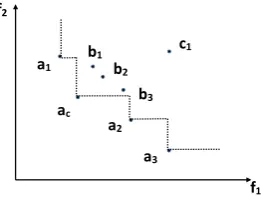
The first situation is depicted in Fig.1, whereacis on the observed Pareto set

com-posed of pointsa1,ac,a2,a3and indicated by the dashed line. Alternativesa1andb1 are the nearest neighbours ofacin the direction of objective f1, and alternativesb3 anda2are the nearest neighbours ofacin the direction of objective f2. We want to

cal-culate the probability that the current Pareto set will change if we allocateτadditional simulation samples toac. If we only allocate samples toac, all other alternatives can

Fig. 2 The Pareto set will change if and only if the estimated mean of alternativeac

will fall outside the shaded area a1

ac

a2

a3

c1

b1

b2

b3

f1

f2

(l1,l2) (u1,l2)

(l1,u2)

(u1,u2)

1. dominates one of the previously non-dominated solutions (a1,a2,a3in Fig.2) 2. becomes dominated itself, or

3. exposes a previously dominated solution (b1,b2,b3in Fig.2).

In the example in Fig.2, a change happens if the new mean estimate falls outside the shaded area.

Since we assume that the samples in the two objectives are independent, we can cal-culate the probability foracto remain in the shaded area separately for each objective,

and multiply them to get the probabilityPthat the new mean estimate foracremains

in the shaded area, and 1−P is the probability that with one additional sample,ac

will move out of the area and hence a new observed Pareto front will be obtained. Let us denote the two objective values of nearest neighbours ofacas(l1,u1)and(l2,u2), i.e.

l1=max{ ¯xpr,1<x¯ac,1|r=1,2, . . . ,k3} l2=max{ ¯xpr,2<x¯ac,2|r=1,2, . . . ,k3} u1=min{ ¯xpr,1>x¯ac,1|r =1,2, . . . ,k3} u2=min{ ¯xpr,2>x¯ac,2|r =1,2, . . . ,k3}

then the probabilityPis

u2

l2 u1

l1

φac,1(x)·φac,2(y)dxdy (2)

where φac,h is the predictive probability distribution of the new location of ac in dimensionh.

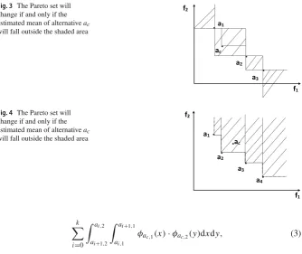
Ifacdoes not expose any new solutions if it is removed, then the Pareto set will only

change if the new estimated mean will become dominated, or dominates a previously non-dominated alternative. Figure3shows an example, with the area in whichacmay

fall without causing a change highlighted.

Assume there arekPareto-optimal alternatives afterachas been removed and they

are sorted from small to large based on f1, with an additional virtual 0th solution at

Fig. 3 The Pareto set will change if and only if the estimated mean of alternativeac

will fall outside the shaded area

a1

ac

f1

f2

a2

a3

Fig. 4 The Pareto set will change if and only if the estimated mean of alternativeac

will fall outside the shaded area a1

a2

a3

a4

ac

f1

f2

k

i=0 ai,2

ai+1,2 ai+1,1

ai,1

φac,1(x)·φac,2(y)dxdy, (3)

where alternativeiwith objective values(ai,1,ai,2)is Pareto optimal ifacis removed.

When ac is not in the Pareto set, a change happens if and only if ac becomes

non-dominated. An example is shown in Fig.4.

In this scenario, the shaded area is defined by all current Pareto optimal alternatives. Similar to the above scenario, if there arekPareto-optimal alternatives, the probability P can be computed as

k

i=1

_∞

ai,2 ai+1,1

ai,1

φac,1(x)·φac,2(y)dxdy (4)

where alternativei is Pareto optimal andak+1,1= ∞.

Based on the above analysis, we can formulate the small-sample multi-objective budget allocation procedure as summarised in Algorithm1.

4.2 M-MOBA indifference-zone procedure

ALGORITHM 1:Procedure M-MOBA PCS

1: Specify a first-stage sample sizen0=5, and a number of samplesτ=1 to allocate per subsequent

stage. Specify stopping rule parameters

2: SampleXi hn,i=1, . . . ,m;h=1, . . . ,H;n=1, . . . ,n0independently, and initialise the

number of samplesni←n0

3: Determine the sample statisticsx¯i,handσˆi2,h, and the observed Pareto front

4:whilestopping rule not satisfieddo

5: For each alternativei, calculate the probabilityPithat the new samples will lead to a change in

the Pareto set

6: Allocateτsamples to the alternative that has the largestPi

7: Update sample statisticsni,x¯i,handσˆi2,hand observe a new Pareto front

8:end while

9: Select alternatives on the observed Pareto front

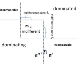
Fig. 5 Indifference-zone definition of Teng et al. (2010) and dominance of a solution relative to solutionm

m

n n’ n’’

Indifference zone δx In

diff

e

re

nc

e zone

δ

y

incomparable

dominang

dominated

indifferent

incomparable

Sect. 2.2.1, one way to deal with this is to introduce an indifference zone, and use the probability of good selection as performance criterion. However, it is not obvi-ous how to define an indifference zone in the case of multiple objectives. In the following, we introduce a new concept of indifference zone and good selection, and develop a corresponding M-MOBA indifference zone (M-MOBA IZ) algo-rithm.

Teng et al. (2010) have proposed an indifference-zone concept for multi-objective problems as follows. A DM is indifferent between system j and system i in objective h, denoted by μj,h μi,h if and only if |δi j h| ≤ δh, where δi j h =

μj,h −μi,h and δh is the indifference zone of the hth objective. Based on this

definition, any solution located within the indifference-zone area of solution m is indifferent to m and so the dominance relationship can be visualised as shown in Fig. 5. PGS has been defined as the probability that exactly all the solutions that are not dominated by any other solution have been identified correctly. How-ever, with this definition small differences can still switch a solution between being in the desired set or not. For example, in the scenario shown in Fig. 5, if solu-tion n is observed as n, it will be incomparable to m, while if it is observed as n it will dominate m. Thus, an algorithm optimising under this definition is likely to spend a lot of simulation samples to distinguish the domination relation-ship between m andn, even if such a small difference may not be relevant to the DM.

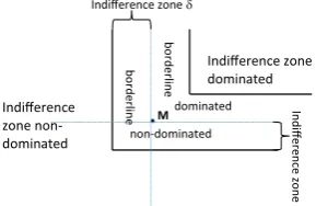
Fig. 6 M-MOBA IZ indifference-zone definition

M

Indifference zone dominated

Indifference zone non-dominated

bo

rd

e

rli

ne

bo

rd

e

rli

ne

dominated

non-dominated

In

d

ifferen

ce zon

e

Indifference zone

4.2.1 New definition of indifference zone and good selection

The key idea of our new indifference-zone definition is to extend the number of cat-egories. Instead of a system being either dominated or non-dominated, we introduce the categories of “indifference-zone dominated”, “borderline non-dominated”, “bor-derline dominated” and “indifference-zone non-dominated” as illustrated by Fig.6. A system is

– indifference-zone dominatedif there is another solution that is at leastδhbetter in

each objectiveh,

– borderline dominated, if it would become non-dominated by improving each objectivehbyδh,

– borderline non-dominated, if it is non-dominated, but would become dominated by worsening each objectivehbyδh,

– indifference-zone non-dominatedif it remains non-dominated even if each objec-tivehis worsened byδh.

More formally,

– solutioni indifference zone dominates solution j, denoted byi ≺I Z j, ifμi,h<

μj,h−δh,∀h =1,2, . . . ,H,

– solutioni borderline dominates solution j, denoted byi I Z j, ifμi,h < μj,h,

∀h=1,2, . . . ,H and∃h∈ {1,2, . . . ,H},|δi j h|δh.

Therefore, a solution j is categorised as

– indifference-zone dominatedif∃i∈ {1,2, . . . ,m},i ≺I Z j,

– borderline dominatedifi ∈ {1,2, . . . ,m},i ≺I Z j and∃i ∈ {1,2, . . . ,m}, i I Z j,

– borderline non-dominatedif i ∈ {1,2, . . . ,m},i ≺I Z j,i ∈ {1,2, . . . ,n}, i I Z jand∃i ∈ {1,2, . . . ,m},h∈ {1,2, . . . ,H}μi,h > μj,h−δh,

– indifference-zone non-dominatedifi ∈ {1,2, . . . ,m},i ≺I Z j ori I Z j and

i∈ {1,2, . . . ,m},h∈ {1,2, . . . ,H}μi,h> μj,h−δh.

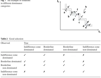
For example, in Fig.7, we have a set of indifference-zone non-dominated solutions a,b,c, which are still Pareto optimal if both objectives increase by a small amount

Fig. 7 An example of solutions in different dominance categories

a b

c d

h

e f

f1

f2

g a’

g’ c’ b’

d’ e’ f’ h’

Table 2 Good selection

Observed True

Indifference-zone dominated

Borderline dominated

Borderline non-dominated

Indifference-zone non-dominated

Indifference-zone dominated

✓ ✓ ✗ ✗

Borderline dominated ✓ ✓ ✓ ✗

Borderline non-dominated

✗ ✓ ✓ ✓

Indifference-zone non-dominated

✗ ✗ ✓ ✓

would still be Pareto dominated even if both objectives are improved byδ, whileg is borderline dominated as it would become non-dominated decreasing its objective values byδ.

Based on the above definitions, we propose a definition of “good selection”. Ifciis

the “true” category of alternativei, we still count the solution as correctly classified if based on the observed objective values, the category is “similar” to the true category, as defined in Table2. For example, we accept if a borderline dominated solution is classified as borderline non-dominated or as dominated, but we do not accept if it is classified as indifference-zone non-dominated. This solves the issue of classifyingn in Fig.5, as there is a tolerance for classification in adjacent categories.

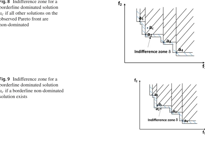
4.2.2 M-MOBA IZ procedure

We use the above definition of PGS to design an M-MOBA procedure that can work with indifference zones (M-MOBA IZ). Similar to the original M-MOBA, we will calculate the probability that a solution, if re-sampled, will change its category by more than one grade. Similar to the M-MOBA PCS procedure, we discuss the calculation of the probability based on the current domination situation of each alternative.

For a solution that is indifference-zone dominated or borderline dominated: – For a solution that is indifference-zone dominated, the area thatacneeds to move

Fig. 8 Indifference zone for a borderline dominated solution

acif all other solutions on the

observed Pareto front are non-dominated

a1

a2

a3

a4

ac

f1

f2

Indifference zone

Fig. 9 Indifference zone for a borderline dominated solution

acif a borderline non-dominated

solution exists a1

a2 a3

a4 ac

f1 f2

Indifference zone

– For a solution that is borderline dominated, if all other solutions on the observed Pareto front are indifference-zone non-dominated, an example for the area thatac

needs to move out is shown in Fig.8, i.e. the original area plus the striped area that allowsacto become borderline non-dominated.

– For a solution that is borderline dominated, if a solution on the observed Pareto front is borderline non-dominated, the area thatacneeds to leave is the area discussed

above plus the small rectangle around the borderline non-dominated solution. For example, if solutiona2shown in Fig.9is borderline non-dominated (with respect toac), the area with indifference zone foracis the shaded part.

For a solution that is on the observed Pareto front and no new solutions become indifference-zone non-dominated or borderline non-dominated when this solution is removed:

– For an indifference-zone non-dominated solution, if all solutions on the observed Pareto front are indifference-zone non-dominated, the area thatacneeds to move

out of is exemplified in Fig.3and the probabilityPcan be calculated with Eq. (3). – For an indifference-zone non-dominated solution, if a solution on the observed Pareto front is borderline non-dominated, the area thatacneeds to move out is the

area in Fig.3plus the stripe areas around the borderline non-dominated solution. Furthermore, if two borderline non-dominated solutions are neighbours on the Pareto front, the small square area between the two stripe areas also needs to be added. For example, in Fig.10,a1anda2are both borderline non-dominated (due toa4anda5, respectively), the areaacthat needs to leave in order to bring a change

is the shaded part shown in Fig.10.

Fig. 10 Indifference zone for an indifference-zone

non-dominated solution if a borderline non-dominated solution exists

a1

ac

f1 f2

a2

a3 a4

a5

Indifference zone

Fig. 11 Indifference zone for a borderline non-dominated solution if all solutions on the observed Pareto front are indifference-zone non-dominated

a1

ac

a2

a3

f1

f2

Indifference zone

Fig. 12 Indifference zone for a borderline non-dominated solution if a borderline

non-dominated solution exists a1

ac

f1

f2

a2

a3

a4

a5

Indifference zone

to move out is shown in Fig,11, which is the original shaded area from Fig.3plus a stripe area on the upper right side.

– For a borderline non-dominated solution, if a solution on the observed Pareto front is borderline non-dominated, the shaded area thatacneeds to leave is the area

discussed in Fig.10plus the stripe area on the upper right side. For example, similar to the situation in Fig.10wherea1anda2are both borderline non-dominated, the area thatacneeds to leave in order to bring a change is the shaded part shown in

Fig.12.

For a solution that is on the observed Pareto front and new solutions become indifference-zone non-dominated or borderline non-dominated when this solution is removed:

Fig. 13 Indifference zone for a solution that, if removed, reveals a set of non-dominated solutions

a1

ac

a2

a3

b1

b2

b3

f1

f2

Indifference zone

c1

Fig. 14 Cells created to compute probability of change

a1

ac

b1

f1

f2

c1

area can be extended accordingly. For example, in Fig.13, sincea2is borderline non-dominated, the area thatacneeds to leave is as the figure shows.

– If the new Pareto-optimal solution after the solution under consideration is removed is borderline non-dominated, the situation is so complex that we have not found a good method to summarise. For this situation, we use a brute-force method that divides the whole plane into different cells based on each solution’s objective values and the indifference zone in each objective accordingly, and checks for each cell whether it would change the current Pareto front in case the currently considered solution were to fall into this cell. For example, if we have four solutions in total as in Fig.14, the number of cells that need to be considered is(4∗3)2=144. Please note that for the sake of clear demonstration, the domination relationship in this figure does not exactly conform to the situation that new Pareto-optimal solution after the solution under consideration is removed is borderline non-dominated.

4.3 M-MOBA hypervolume procedure

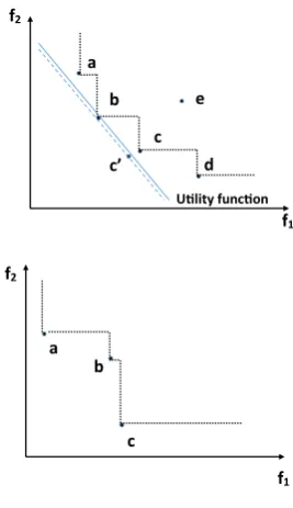
Fig. 15 Even though all dominance relations are correct if solutioncis observed asc, the DM may pick the wrong solution

a

b

f1

f2

c

d c’

e

Ulity funcon

Fig. 16 Solutionsaandcare more likely to be preferred by a DM

a b

f1

f2

c

by a DM than solutionb, since they are much better thanbin one objective but just a little worse in the other objective. So, misclassifyingb is probably not as bad as misclassifyingaandc, but PCS does not make this distinction.

Given these drawbacks of the PCS measure for multi-objective problems, we pro-posehypervolume difference(HVD) as an alternative measure.

LetΛdenote the Lebesgue measure, then the hypervolume (HV) is defined as

H V(B,R):=Λ ⎛ ⎝

y∈B

{y| y≺y≺R} ⎞

⎠_, B⊆Rm (5)

where B is a set of solutions and R ∈ Rm denotes a reference point that is usually user defined and chosen such that it is dominated by all other solutions. Figure17

shows a set of five alternatives in 2-objective space. Three of the solutions are Pareto-optimal, and the HV is the shaded area, defined by the Pareto-optimal solutions and the reference pointR. The dominated solutions do not contribute to the HV. HV is a standard metric to judge the performance in multi-objective optimisation. It rewards solutions close to the true Pareto front, as well as a good spread of solutions along the true Pareto front (Beume et al.2007).

But for the case of ranking and selection where evaluations are stochastic, we need a metric that penalises over-estimation as well as under-estimation of objective values, and thus propose the hypervolume difference (HVD). Given two sets of Pareto-optimal solutionsAandB,

Fig. 17 Hypervolume of a set of solutions

a

b

c

d

R

f1

e f2

Fig. 18 Hypervolume difference

of two sets of solutions a

b

c

d

R

a’

f1

b’

d’ e

c’ f2

Fig. 19 Hypervolume difference penalises any deviation from the

true front _a

b

f1

f2

c d c’

e

Figure18provides an example for the proposed HVD.

HVD is able to overcome the drawbacks of PCS-based metrics discussed above. For the scenario shown in Fig.15, HVD will penalise deviations from the true fitness values of Pareto-optimal solutions, even if all dominance relations are correct, see Fig.19. And for the scenario shown in Fig.16, while PCS fails to reflect the higher importance ofaandc, hypervolume does pay more attention to these solutions. This is illustrated in Fig.20: If distorting solutionsaandbby the same distance and direction, the HVD between the new and old Pareto front made by a distortion toais larger than by the same distortion tob.

Fig. 20 Hypervolume change caused by different solutions is different

a b

f1

f2

c b’

Hypervolume change caused by b

c’

Hypervolume change caused by c

Fig. 21 Effect of choosing reference point

a

b

f1

f2

d c

R

Following the general M-MOBA framework, we will sample where we expect the sample will lead to the biggest change in HV, i.e. where the expected HVD between the Pareto fronts before and after sampling is maximal.

4.3.1 Mathematical calculation of the expected HV change

Calculating the expected HV change requires to break down the calculation into differ-ent cells, but for each cell, we can find a closed form expression. Then, these expected changes can be added up to result in the overall expected HV change. In the following, we will explain the computation for one particular cell, with other cells computed analogously. Some examples for how a move of one solution will influence the HVD can be found in Branke et al. (2016).

Consider Fig. 22, where all solutions on the current Pareto front are labelled a1, . . . ,ak, with coordinatesai,h for alternativei and objectiveh, and the solutions

are sorted in increasing order of objective 1. For technical reasons, let us define a0,1 = −∞,a0,2 = ar,2,ak+1,1 = ar,1,ak+1,2 = −∞. We consider another sample for design ac, and the calculation for one particular cell that is outlined

in bold and defined by upper right corner u with coordinates (u1,u2) and lower left corner l with coordinates (l1,l2). Let us assume that these two corners are defined by the Pareto-optimal solutions ap and aq, by u = (ap+1,1,aq−1,2) and l=(ap,1,aq,2).

Fig. 22 Different cells that need to be considered when calculating the expected HV

change from re-sampling a1

R f2 f1 a2 a4 ac a’c l u b1 b2 b3 b4 (p) (q) u2 l2 u1 l1 ⎡

⎣₍ap₊1_,1−x)(ap_,2−y)+

p<i<q

(ai₊1_,1−ai_,1)(ai_,2

−y)]·φc,1(x)·φc,2(y)dxdy (7)

whereφc,his the predictive probability distribution of the new location ofxcin

dimen-sionh.

For efficient computation, we derive a closed form for calculating the expected HV change in one cell. Letφ(x;μ, κ, ν)denote the distribution ofμ+√1_κT_ν, whereT_ν is a random variable with standardt distribution withνdegrees of freedom, i.e. the t distribution we estimate for the new location of an alternative’s mean values after having taken another sample, with meanμ, precisionκandνdegrees of freedom. The cumulative density function is then

(x;μ, κ, ν)= t(

√

κ(x−μ);ν) (8)

with t(x;ν)the cumulative standardt-distribution, and the probability density

func-tion is

φ(x;μ, κ, ν)=√κ·φt(

√

κ(x−μ);ν)=

κ νπ

Γ (ν+1

2 )

Γ (ν

2)

·

1+κ(x−μ) 2

ν

−ν+1 2

(9)

withφt(x;ν)the standard t-distribution. The HV change, due to the point we are

considering moving to a new position(x,y), is always a function in the formax y+ bx+cy+d. The constant coefficientsa,b,c,dare different in different areas, and some of the coefficients could be 0 sometimes. The contribution of the area[l1,u1]×[l2,u2] (e.g. the small cell highlighted in Fig.22) to the expectation of the HV change is

u1

l1 u2

l2

(ax y+bx+cy+d)·φi,1(x)·φi,2(y)dxdy

=a u1

l1

xφi,1(x)dx u2

l2

yφi,2(y)dy+b· i,2(y)|_lu₂2· u1

l1

xφi,1(x)dx

+c· i_,1(x)|u_l11 · u2

l2

where φi,h(x) = φ(x;μi,h, κi,h, νi), i,h(x) = (x;μi,h, κi,h, νi),μi h = ¯xi,h,

κi,h = ni(ni +τi)/τiσˆ_i2_,h and νi = ni −1. On the right-hand side of Eq. (10),

the most critical part is solving the integrals, and it can be done by calculating the corresponding indefinite integral, which is

xφ(x;μ, κ, ν)dx=

(x−μ)φ(x;μ, κ, ν)dx+μ (x;μ, κ, ν)dx

=ψ(x;μ, κ, ν)+μ (x;μ, κ, ν)

(11)

with

ψ(x;μ, κ, ν):=

(x−μ)φ(x;μ, κ, ν)dx

=

ν κπ ·

Γ (ν+1

2 )

(1−ν)Γ (ν₂)

1+κ(x−μ) 2

ν

1−ν

2

=ν+κ(x−μ)2

(1−ν)√κ φ(x;μ, κ, ν).

(12)

In the rest of this section, for convenience, we will denoteψ(x;μi h, κi h, νi)asψi h(x).

Using the above results and gathering the terms with same integrals, Eq. (10) can be rewritten as

u1

l1 u2

l2

(ax y+bx+cy+d)·φi_,1(x)·φi_,2(y)dxdy

=ai,1(x)|u_l11i,2(y)|u_l22 +(b+aμi,2)i,1(x)|u_l11 i,2(y)|_lu₂2

+(c+aμi_,1) i_,1(x)|u_l11i_,2(y)|u_l22+(aμi_,1μi_,2+bμi_,1

+cμi,2+d) i,1(x)|ul11 i,2(y)|

u2

l2,

(13)

where is the integral ofψ.

For example, considering the integral (7), we will have

a =1, b= −ap,2, c= −ap₊1_,1−

p<i<q

(ai₊1_,1−ai_,1), d =ap₊1_,1ap_,2+

p<i<q

(ai₊1_,1−ai_,1)ai_,2,

and then, we can substitute them, in addition to

μc,h= ¯xc,h, κc,h =nc(nc+τc)/τcσˆc2,h, νc=nc−1,

whereh =1 or 2, into Eq. (13) to solve the integral (7).

sample to alternativeiand allocateτ samples to the alternativei that has the largest expected hypervolume change.

4.4 M-MOBA procedure for differential sampling between the objectives

Sometimes, objectives can be evaluated independently, e.g. if different simulation models are used to evaluate different criteria. In this case, in order to further improve the efficiency of sampling, it is possible to regard the sampling allocation process for each objective independently. This independent sampling procedure can be employed with different measures and without loss of generality we use PCS in this paper. Instead of evaluating all objectives of an alternative simultaneously as in the M-MOBA PCS procedure, we will evaluate only one objective of one alternative in each iteration. We calculatePiusing the same methods as in M-MOBA PCS, and allocate the simulation

sample to the solution and objective that has the biggest probability to change the cur-rent Pareto front. For comparison purposes, for a 2-objective problem, we assume the M-MOBA PCS procedure will allocate one sample for each objective of a solution in every iteration, while the M-MOBA Differential Sampling PCS (M-MOBA DS PCS) procedure will only allocate one sample to the selected objective. Empirical results in Sect.5show that by allowing to evaluate objectives independently, the efficiency of the algorithm may be improved substantially. This would be even more the case if evalu-ating different objectives would take different times or involve different costs, because it would allow the algorithm to focus on the cheaper objectives. Different costs could be easily integrated into M-MOBA DS PCS by using the quotient of probability of change and computational cost to decide which solution and objective to evaluate next.

5 Empirical results and analysis

In this section, we present empirical experiments using different M-MOBA methods and compare their performance with Equal allocation (which simply allocates an equal number of samples to each alternative) according to different performance measures. For each method, each design is sampled n0 = 5 times during initialisation, and additional samples are allocated one at a time (τ = 1) until a pre-set budget has been used up. All results are averaged over 1000 runs. We report the performance of M-MOBA PCS, M-MOBA IZ, M-MOBA HV and M-MOBA DS PCS.

Table 3 True expected performance in each objective, SD in all cases is 5

Index Obj. 1 Obj. 2

0 1 2

1 3 1

2 5 5

Fig. 23 Comparison of P(CS) for different algorithms on the 3-alternative case

5.1 M-MOBA PCS procedure

In an earlier paper (Branke and Zhang2015), we compared the performance of M-MOBA PCS with MOCBA (Chen and Lee2010) by using two configurations from Chen and Lee (2010). In Branke and Zhang (2015), as we did not have access to an implementation of MOCBA at the time, we just compared with results read approx-imately from figures provided in Chen and Lee (2010). For this paper, Dr. Haobin Li has kindly provided us with his code of MOCBA, and so we are able to compare MOCBA PCS and M-MOBA directly and under identical settings.

In the first benchmark problem, there are three designs and each of them is evaluated according to two objectives. Objective values of the designs are shown in Table3.

The resulting P(CS) over the budget allocated is shown in Fig.23. As can be seen, our algorithm obtains a significantly higher P(CS) than Equal allocation with the same simulation budget. M-MOBA PCS performs very similar to MOCBA on this problem. The second configuration has 16 alternatives, and the objective values of each design are shown in Table4and visualised in Fig.24.

Table 4 Standard configuration with 16 alternatives and two objectives. Standard deviation for all designs is 2 in each objective

Index Obj. 1 Obj. 2 Index Obj. 1 Obj. 2

1 0.5 5.5 9 4.8 5.5

2 1.9 4.2 10 5.2 5

3 2.8 3.3 11 5.9 4.1

4 3 3 12 6.3 3.8

5 3.9 2.1 13 6.7 7.2

6 4.3 1.8 14 7 7

7 4.6 1.5 15 7.9 6.1

8 3.8 6.3 16 9 9

Fig. 24 Standard configuration with 16 alternatives

Fig. 25 Comparison of P(CS) for different algorithms on the 16-alternative case

Fig. 26 Similar solution configuration with 13 alternatives

Table 5 Configuration with 13 alternatives and two objectives. Standard deviation for all designs is 1.5 in each objective

Index Obj. 1 Obj. 2 Index Obj. 1 Obj. 2 Index Obj. 1 Obj. 2

1 1 8 6 3 7 11 2.6 3.9

2 2 5 7 3.05 2.2 12 2 7

3 3.5 5.01 8 1.5 6 13 2.5 6

4 3 2 9 2.1 5.2

5 2.5 8 10 2.5 4

Fig. 27 Similar solution configuration PCS performance comparison

5.2 M-MOBA IZ procedure

Fig. 28 Similar solution configuration PGS performance comparison

Fig. 29 Allocation of samples to different alternatives for 13 similar alternatives configuration

Fig. 30 Comparison of relative hypervolume difference for standard configuration with 16 alternatives

Table 6 Borderline configuration with ten alternatives and two objectives. Standard deviation for all designs is 2 in each objective

Index Obj. 1 Obj. 2 Index Obj. 1 Obj. 2

1 1 5 6 4 2.1

2 5 1 7 2.1 4

3 3 3 8 5.5 5

4 3.1 2 9 3.5 5

5 2 3.1 10 6 6

5.3 M-MOBA HV procedure

In Branke et al. (2016), we tested three configurations, and compared them with two other methods, the M-MOBA PCS (Branke and Zhang2015) and Equal allocation. The test results in this section are taken from Branke et al. (2016) and are repeated here for completeness. The first configuration is still the 16 alternatives configuration proposed by Chen and Lee (2010). Figure30reports the reduction in the HV difference as the number of samples allocated increases. It can be seen that the M-MOBA-HV method works much better than both the Equal and M-MOBA PCS methods in terms of HVD between the selected and true Pareto set. Although M-MOBA PCS has been shown to identify the Pareto-optimal solutions much more quickly than Equal allocation on this problem (Branke and Zhang2015), in terms of HVD it is actually only slightly better than Equal allocation.

Fig. 31 Borderline configuration with ten alternatives

Fig. 32 Comparison of relative hypervolume difference of borderline configuration

The result is shown in Fig.32. Again, M-MOBA-HV works very well. The PCS-based version of M-MOBA now is even worse than Equal allocation. To investigate this further, Fig.33shows the percentage of samples allocated to a particular design. M-MOBA PCS allocates quite a few samples to the borderline designs 3, 6 and 7, because it aims to improve the probability of correct selection, and for these designs the classification is most difficult. For a decision maker, however, these designs are probably less relevant. M-MOBA-HV instead focuses on the designs 1, 2, 4 and 5, which are the Pareto-optimal solutions probably most relevant to a decision maker. Thus, it creates reliable performance estimates where it is most relevant.

Fig. 33 Allocation of samples to the different alternatives for borderline configuration

Table 7 Similar solution configuration with eight alternatives and two objectives. Standard deviation for all designs is 2 in each objective

Index Obj. 1 Obj. 2

1 1 5

2 5 1

3 3.2 2.1

4 3 2

5 2 3.1

6 6 4

7 5 5

8 4 6

Fig. 34 Similar solution configuration with eight alternatives

2 in the sense that M-MOBA-HV works best, and the PCS-based M-MOBA is worse than Equal allocation. Again, Fig.36provides further detail on the distribution of samples onto the different alternatives.

Fig. 35 Comparison of relative hypervolume difference of similar solution configuration

Fig. 36 Allocation of samples to the different alternatives for similar solution configuration

Fig. 37 Hypervolume difference depending on the number of samples taken, averaged over 1000 random configurations

0 50 100 150 200 250 300 350 400

budget 5

10 15 20

relative hypervolume difference

Equal M-MOBA HV M-MOBA PCS

dimension. Algorithms are tested once on each of the 1000 random configurations, and results are averaged over these 1000 runs.

Fig. 38 P(CS) depending on the number of samples taken, averaged over 1000 random configurations

0 50 100 150 200 250 300 350 400

budget

0.3 0.35 0.4 0.45 0.5 0.55 0.6 0.65 0.7 0.75 0.8

P(CS)

Equal M-MOBA HV M-MOBA PCS

Table 8 Time required per sample allocation

Number of alternatives Best Worst Average

10 0.079110s 0.093693s 0.083943s

20 0.099771s 0.11613s 0.106111s

50 0.239546s 0.399704s 0.259820s

100 0.497097s 0.585236s 0.515388s

not care about some borderline solutions, as these solutions do not contribute to the HV. The experiment on randomly generated configurations reinforces our intuition that the selection of the algorithm should depend on the chosen performance measure. Finally, the timings reported in Table8approximate the time it takes to perform one sample allocation with M-MOBA HV (the slowest of the algorithm variants proposed in this paper). We report the shortest, longest and average wall-clock time of 100 times running with MATLAB 2018b on a machine with 2.4 GHz Intel Core i7 CPU and 8GB memory. The average computational time is almost exactly linear in the number of alternatives.

5.4 M-MOBA DS PCS procedure

Still using the 16 alternatives configuration used in Chen and Lee (2010), we test the M-MOBA DS PCS procedure and compare it with the original M-MOBA PCS procedure and Equal allocation.

Fig. 39 M-MOBA DS PCS procedure

0 500 1000 1500

budget

0 0.1 0.2 0.3 0.4 0.5 0.6

P(CS)

Equal M-MOBA DS PCS M-MOBA PCS

Table 9 Different purposes _{Purpose Method}

Minimise PCS M-MOBA PCS

Minimise PCS but ignore small differences M-MOBA IZ

Any performance measure, but if objective functions are derived from different simulation models independently

M-MOBA DS

Minimise hypervolume difference M-MOBA HV

6 Conclusion

In this paper, we presented an overview on the M-MOBA method for ranking and selection in case of two objectives. We show how this method can be adapted to various different scenarios such as the case of an indifference zone, hypervolume as performance criterion, or the case where objectives can be evaluated independently, and we propose new variants and evaluation criteria. Empirical results show M-MOBA is able to substantially reduce the number of simulation runs needed to obtain a desired performance, when compared to equal allocation or other methods from the literature. In conclusion, we suggest different M-MOBA variants are used in different situa-tions according to Table9.

There are several avenues for future research, including a test on real-world simu-lation optimisation problems, other M-MOBA variants with different stopping rules rather than fixed budget, considering the situation when the objectives are correlated and a development of an M-MOBA variant that works with more than two objectives.

Acknowledgements We thank Mr. Yang Tao, PhD student at the University of Nottingham, for his signif-icant contribution to the M-MOBA HV method.

References

Andradottir S, Kim SH (2010) Fully sequential procedures for comparing constrained systems via simula-tion. Nav Res Logist 57(5):403–421

Bader J, Zitzler E (2011) Hype: an algorithm for fast hypervolume-based many-objective optimization. Evol Comput 19(1):45–76

Beume N, Naujoks B, Emmerich M (2007) SMS-EMOA: multiobjective selection based on dominated hypervolume. Eur J Oper Res 161(3):1663–1669

Birattari M, Yuan Z, Balaprakash P, Stützle T (2010) F-race and iterated f-race: an overview. In: Bartz-Beielstein T, Chiarandini M, Paquete L, Preuss M (eds) Experimental methods for the analysis of optimization algorithms. Springer, Berlin, pp 311–336

Branke J, Chick S, Schmidt C (2007) Selecting a selection procedure. Manag Sci 53(12):1916–1932 Branke J, Chick S, Schmidt C (2005) New developments in ranking and selection: an empirical comparison

of the three main approaches. In: Winter simulation conference. IEEE, pp 708–717

Branke J, Gamer J (2007) Efficient sampling in interactive multi-criteria selection. In: INFORMS simulation society research workshop, pp 42–46

Branke J, Zhang W (2015) A new myopic sequential sampling algorithm for multi-objective problems. In: Winter simulation conference. IEEE, pp 3589–3598

Branke J, Zhang W, Tao Y (2016) Multiobjective ranking and selection based on hypervolume. In: Winter simulation conference. IEEE, pp 859–870

Butler J, Morrice D, Mullarkey P (2001) A multiple attribute utility theory approach to ranking and selection. Manag Sci 47(6):800–816

Chau M, Fu M, Qu H, Ryzhov I (2014) Simulation optimization: a tutorial overview and recent developments in gradient-based methods. In: Winter simulation conference. IEEE, pp 21–35

Chen CH (1996) A lower bound for the correct subset-selection probability and its application to discrete-event system simulations. IEEE Trans Autom Control 41(81):1227–1231

Chen CH, Lee LH (2010) Stochastic simulation optimization: an optimal computing budget allocation. World Scientific, New York

Chick S, Inoue K (2001) New two-stage and sequential procedures for selecting the best simulated system. Oper Res 49(5):732–743

Chick S, Wu Y (2005) Selection procedures with frequentist expected opportunity cost bounds. Oper Res 53(5):867–878

Chick S, Branke J, Schmidt C (2010) Sequential sampling to myopically maximize the expected value of information. INFORMS J Comput 22(1):71–80

DeGroot M (2005) Optimal statistical decisions, vol 82. Wiley, New York

Feldman G, Hunter SR (2018) Score allocations for bi-objective ranking and selection. ACM Trans Model Comput Simul (TOMACS) 28(1):7

Feldman G, Hunter SR, Pasupathy R (2015) Multi-objective simulation optimization on finite sets: optimal allocation via scalarization. In: Winter simulation conference. IEEE, pp 3610–3621

Frazier P (2014) A fully sequential elimination procedure for indifference-zone ranking and selection with tight bounds on probability of correct selection. Oper Res 62(4):926–942

Frazier P, Powell W, Dayanik S (2008) A knowledge-gradient policy for sequential information collection. SIAM J Control Optim 47(5):2410–2439

Frazier P, Kazachkov K (2011) Guessing preferences: A new approach to multi-attribute ranking and selection. In: Winter simulation conference. IEEE, pp 4319–4331

Fu M, Hu JQ, Chen CH, Xiong X (2007) Simulation allocation for determining the best design in the presence of correlated sampling. INFORMS J Comput 19(1):101–111

Fu M, Chen CH, Shi L (2008) Some topics for simulation optimization. In: Winter simulation conference. IEEE, pp 27–38

Gittins J, Glazebrook K (2011) Multi-armed bandit allocation indices. Wiley, New York

He D, Chick S, Chen CH (2007) The opportunity cost and ocba selection procedures in ordinal optimization for a fixed number of alternative systems. IEEE Trans Syst Man Cybern Part C Appl Rev 37(5):951–961 Hunter SR, Feldman G (2015) Optimal sampling laws for bi-objective simulation optimization on finite

sets. In: Winter simulation conference. IEEE, pp 3749–3757

Hunter SR, Applegate EA, Arora V, Chong B, Cooper K, Rincon-Guevara O, Vivas-Valencia C (2019) An introduction to multiobjective simulation optimization. ACM Trans Model Comput Simul 29(1):7:1– 7:36

Keeney RL, Raiffa H (1993) Decisions with multiple objectives: preferences and value trade-offs. Cambridge University Press, Cambridge

Kim SH, Nelson BL (2006) Chapter 17 Selecting the best system. In: Henderson SG, Nelson BL (eds) Handbooks in operations research and management science, vol 13. Elsevier, pp 501–534

Lee LH, Chew EP, Teng S (2007) Finding the Pareto set for multi-objective simulation models by mini-mization of expected opportunity cost. In: Winter simulation conference, pp 513–521

Lee LH, Chew EP, Teng S (2010a) Computing budget allocation rules for multi-objective simulation models based on different measures of selection quality. Automatica 46(12):1935–1950

Lee LH, Chew EP, Teng S, Goldsman D (2010b) Finding the non-dominated pareto set for multi-objective simulation models. IIE Trans 42(9):656–674

Lee S, Nelson B (2015) Computational improvements in bootstrap ranking & selection procedures via multiple comparison with the best. In: Winter simulation conference. IEEE, pp 3758–3767 Mattila V, Virtanen K (2015) Ranking and selection for multiple performance measures using incomplete

preference information. Eur J Oper Res 242:568–579

Morrice D, Butler J (2006) Ranking and selection with multiple targets. In: Winter simulation conference. IEEE, pp 222–230

Morrice D, Butler J, Mullarkey P (1998) An approach to ranking and selection for multiple performance measures. In: Winter simulation conference, pp 719–726

Park C, Kim SH (2011) Handling stochastic constraints in discrete optimization via simulation. In: Winter simulation conference, pp 4217–4226

Pasupathy R, Hunter SR, Pujowidianto NA, Lee LH, Chen C (2014) Stochastically constrained ranking and selection via SCORE. ACM Trans Model Comput Simul 25(1):1–26

Pujowidianto NA, Pasupathy R, Hunter S, Lee LH, Chen CH (2012) Closed-form sampling laws for stochas-tically constrained simulation optimization on large finite sets. In: Winter simulation conference. IEEE, pp 1–10

Ryzhov I, Powell W, Frazier P (2012) The knowledge gradient algorithm for a general class of online learning problems. Oper Res 60(1):180–195

Shahriari B, Swersky K, Wang Z, Adams RP, de Freitas N (2016) Taking the human out of the loop: a review of bayesian optimization. Proc IEEE 204(1):148–175

Teng S, Lee L, Chew EP (2010) Integration of indifference-zone with multi-objective OCBA. Eur J Oper Res 203:419–429

Wan W, Wang H (2017) Sequential probability ratio testing for multiple-objective ranking and selection. In: Winter simulation conference. IEEE, pp 1998–2009

Zhang T, Georgiopoulos M, Anagnostopoulos G (2017) Pareto-optimal model selection via SPRINT-race. IEEE Trans Cybern 48(2):596–610

Zhang T, Georgiopoulos M, Anagnostopoulos G (2013) S-race: a multi-objective racing algorithm. In: Genetic and evolutionary computation conference. ACM, pp 1565–1572

Zhang T, Georgiopoulos M, Anagnostopoulos GC (2015) Sprint multi-objective model racing. In: Genetic and evolutionary computation conference. ACM, pp 1383–1390

Zitzler E, Thiele L (1999) Multiobjective evolutionary algorithms: a comparative case study and the strength pareto approach. IEEE Trans Evol Comput 3(4):257–271

Zitzler E, Thiele L, Laumanns M, Fonseca C, Grunert FV (2003) Performance assessment of multiobjective optimizers: an analysis and review. IEEE Trans Evol Comput 7(2):117–132