Classification of two and three factor time homogeneous separable LMMs

warwick.ac.uk/lib-publications

Original citation:

Gogala, Jaka and Kennedy, Joanne E.. (2017) Classification of two-and three-factor time-homogeneous separable LMMs. International Journal of Theoretical and Applied Finance, 20 (2). 1750021.

Permanent WRAP URL:

http://wrap.warwick.ac.uk/87823

Copyright and reuse:

The Warwick Research Archive Portal (WRAP) makes this work by researchers of the University of Warwick available open access under the following conditions. Copyright © and all moral rights to the version of the paper presented here belong to the individual author(s) and/or other copyright owners. To the extent reasonable and practicable the material made available in WRAP has been checked for eligibility before being made available.

Copies of full items can be used for personal research or study, educational, or not-for-profit purposes without prior permission or charge. Provided that the authors, title and full

bibliographic details are credited, a hyperlink and/or URL is given for the original metadata page and the content is not changed in any way.

Publisher’s statement:

Electronic version of an article published as International Journal of Theoretical and Applied Finance, 20 (2). 1750021. http://dx.doi.org/10.1142/S0219024917500212 © copyright World Scientific Publishing Company http://www.worldscientific.com/

A note on versions:

The version presented here may differ from the published version or, version of record, if you wish to cite this item you are advised to consult the publisher’s version. Please see the ‘permanent WRAP URL’ above for details on accessing the published version and note that access may require a subscription.

Classification of Two- and Three-Factor

Time-Homogeneous Separable LMMs

Jaka Gogala

and Joanne E. Kennedy

1

Department of Statistics, University of Warwick

Coventry, CV4 7AL, United Kingodm

23rd January 2017

Abstract

The flexibility of parameterisations of the LIBOR market model comes at a cost, namely the LIBOR market model is high-dimensional, which makes it cumbersome to use when pricing derivatives with early exercise features. One way to overcome this issue for short and medium term time-horizons is by imposing the separability condition on the volatility functions and approximating the model using a single time-step approximation.

In this paper we examine the flexibility of separable LIBOR market models under the relaxed assumption that the driving Brownian motions can be correlated. In particular, we are interested in how the separability condition interacts with time-homogeneity – a desirable property of a LIBOR market model. We show that the two concepts can be related using a Levi-Civitá equation and provide a characterization of two- and three-factor separable and time-homogeneous LIBOR market models and show that they are of practical interest. The results presented in this paper are also applicable to local-volatility LIBOR market models. These separable volatility structures can be used for the driver of a two- or three-dimensional Markov-functional model - in which case no (single time step) approximation is needed and the resultant model is both time-homogeneous and arbitrage-free.

Keywords: Levi-Civitá equation, LIBOR market model, Markov-functional models, separability, time-homogeneity.

1

Introduction

The LIBOR Market Models (LMMs) are one of the most popular classes of terms structure models. One of the reasons for their popularity can be attributed to the flexibility of their parameterisations. However, this flexibility comes with a major drawback, the Markovian dimension of a LMM is equal to the number of forward rates in the model. This makes them particularly cumbersome to use for pricing of derivatives with early exercise features.

To overcome the issue of high-dimensionality Pietersz et al. (2004) proposed theseparability constraint on the volatility structure of the LMM and proved that

a separable LMM has an approximation with Markovian dimension equal to the number of Brownian motions driving the model dynamics. This process came with two drawbacks. Firstly, it greatly restricted the class of available parameterisations. In particular, it was noted in Joshi (2011) that the separability condition is too restrictive to use when the instantaneous volatilities are time-homogeneous. Secondly, the approximation obtained is not arbitrage free and is only useful for time horizons up to 15 years.

In this paper we mainly address the first issue. In particular, we characterise two- and three-factor separable parameterisations of the LMM when components of the Brownian motion driving the model’s dynamics are allowed to be correlated. We then analyse the obtained parameterisations and show that they are of practical interest.

We briefly comment on the second issue by pointing out the relationship between the separable LMMs to the Markov-functional models (MFMs) (Hunt et al., 2000). In particular, the characterised parameterisations can be used to define two- and three-dimensional MFMs that can be implemented efficiently and are arbitrage-free. Furthermore, we note that the ideas presented here can be extended to a more general class of local-volatility LMMs (Andersen and Andreasen, 2000).

The remainder of the paper is structured as follows. In Section 2 we introduce the basic concepts of LMMs. The separability condition is discussed and generalised in Section 3. In Section 4 we characterise the two- and three-factor separable LMM with time-homogeneous instantaneous volatilities. In Section 5 we discuss the models obtained from a practical point of view. Section 6 concludes.

2

LIBOR Market Models

Throughout the paper we will assume we are working on a filtered probability space (Ω,_F,_{Ft}t≥0,P) supporting a Brownian motion and satisfying the usual conditions. We will be interested in a single currency economy consisting of zero-coupon bonds (ZCBs) maturing on datesT1< . . . < Tn+1 and will denote the time t_≤ Ti, i = 1, . . . , n+ 1, price of a Ti-maturity ZCB by Dt,Ti. We will model the

prices of ZCBs indirectly via the forward LIBORsLi, i= 1, . . . , n, defined by

Li_t= Dt,Ti−Dt,Ti+1

αiDt,Ti+1

, t_≤Ti, i= 1, . . . , n, (2.1)

where αi is the accrual factor associated with the period [Ti, Ti+1].

Over the last few years, since the financial crisis of 2008, the interest-rate markets have evolved and it is now no longer sufficient to assume that equation (2.1) provides an accurate representation of the connection between discount factors and LIBORs. We now live in a ‘multi-curve’ world where discounting is usually driven by overnight index swaps (OIS) (since collateral deposits usually receive interest based on overnight rates) and LIBORs are correctly treated as separate. In the context of a term-structure model there are various levels of sophistication one could adopt in generalising (2.1). The simplest, which is sufficient for most applications in practice, would be to take

Li_t−Dt,Ti−Dt,Ti+1

αiDt,Ti+1

=si_t, t≤Ti, i= 1, . . . , n, (2.2)

For the purposes of this paper we will stick with the definition (2.1), for ease of exposition, but remark that extending our results to (2.2) whensi_t is non-stochastic is straightforward.

Amongst the most popular models of the described economy is the LIBOR Market Model (LMM). It was developed in the 1990s by Miltersen et al. (1997), Brace et al. (1997), Musiela and Rutkowski (1997) and Jamshidian (1997). The basic idea behind the LMM is that the process (Li_t)_t∈[0,Ti]is a log-normal martingale

under the Ti+1-forward measure associated with the Ti+1-maturity ZCB as the numeraire. In particular the prices of caplets on each of the forward LIBORs are given by the Black (1976) formula. To fully specify a LMM we need to specify the joint dynamics of the forward LIBORs under a common equivalent martingale measure (EMM).

A d-factor LMM under the Tn+1-forward measure, usually referred to as the terminal measure, is given by a system of SDEs

dLi_t=Li_thσ˜i(t), dWt˜ i −Li_t n

X

j=i+1

αjLj_thσ˜i(t),σ˜j(t)i

1 +αjLj_t dt, t≤Ti, i= 1, . . . , n, (2.3)

where ˜W is a standardd-dimensional standard Brownian motion under the measure

Fn+1and ˜σi : [0, Ti]→Rd, i= 1, . . . , n, are bounded measurable functions andhx, yi denotes the inner product of vectors. One can show that under these conditions the system of SDEs (2.3) admits a strictly positive strong solution when the initial forward LIBORs Li₀, i= 1, . . . , n, are strictly positive (see Section 14.2 in Andersen and Piterbarg (2010) for more details).

The specification of a LMM as in (2.3) is particularly useful from a computational perspective. For example it allows for a straight-forward implementation via Monte Carlo methods. However, it offers little intuition about the model’s dynamics. It is therefore often useful to introduce instantaneous volatility and instantaneous correlation functions. The instantaneous volatility functions are given by

σinst,i(t) =

q

hσ˜i_(t),σ˜i_{(t)i, t≤T}

i, i= 1, . . . , n, (2.4)

and the instantaneous correlation functions are given by

ρinst_i,j (t) = hσ˜

i_(t),σ˜j_(t)i

σinst,i_(t)σinst,j_(t), t≤Ti∧Tj, i, j = 1, . . . , n. (2.5)

It is easy to see that

d(logLi_t)d(logLj_t) =ρinst_i,j (t)σinst,i(t)σinst,j(t)dt, t_≤Ti∧Tj, i, j= 1, . . . , n, (2.6)

and one can show that the instantaneous volatility and correlation functions uniquely determine a LMM. Furthermore, the timet_≤Ti implied volatility of a caplet written on Li_Ti is a deterministic function given by

σimpl,i(t) = √ 1

Ti−t

Z Ti

t

σinst,i(s)2ds

1₂

, t≤Ti, i= 1, . . . , n. (2.7)

It is often convenient to fix a calendar time t and consider the time t implied volatilities as a function of the maturity of the caplet, i.e.

Ti 7→σimplt ,i, Ti > t. (2.8)

Observe that by specifying the instantaneous volatility functions one implicitly specifies the evolution of the term structure of volatilities over time. In practice one often does not have a particular view on the dynamics of volatility surface and is faced with two natural choices. Either he chooses the implied volatilities to be constant functions of time (i.e. depend only on the maturity of the caplet) or that the implied volatilities are a function of the time to maturity (i.e. depend on the differenceTi−t) (see Section 6.2 in Rebonato (2002)). In this paper we will focus on the latter choice. It is easy to see that the implied volatility of a caplet will depend on the time to maturity if the instantaneous volatility functions satisfy the

time-homogeneity condition

σinst,i(t) =σinst(Ti−t), t≤Ti, i= 1, . . . , n, (2.9)

whereσinst : [0, Tn]_→R+ is some bounded measurable function. In particular,σinst is often taken to be of the form

σinst(Ti−t) = a+b(Ti−t)

exp ₋c(Ti−t)

+d. (2.10)

This parameterisation was proposed by Rebonato (1999) and remains a popular choice amongst practitioners.

Let us now turn our attention back to the specification of the LMM. Recall that we assumed that the d-dimensional Brownian motion ˜W has independent components. While this assumption is in general non-restrictive, it turns out to be beneficial to relax it when there are additional constraints associated with functions ˜

σi, i= 1, . . . , n.

Suppose that ρ : [0, Tn] _{→ R}d×d is a continuous matrix valued function such that ρ(t) is a full rank correlation matrix fort_≤Tn.Then there exists a continuous matrix valued function R : [0, Tn]_→Rd×d such thatR(t) is positive definite and R(t)R(t) =ρ(t) fort_≤Tn. Then we can define a d-dimensional Brownian motion W (with correlated components) by

Wt=

Z t

0 R(s)d ˜

Ws, t≤Tn, (2.11)

and clearly dW_tTdWt = R(t)R(t)dt = ρ(t)dt. Now we can define functions σi : [0, Ti]→Rd by

σi(t) =R(t)−1σ˜i(t), t_≤Ti, i= 1, . . . , n. (2.12) Observe that _hσ˜i(t),Wt˜ i=_hσi(t), dWti and _hσ˜i(t),σ˜j(t)i=_hσi(t), ρ(t)σj(t)i. Then if (L1, . . . , Ln) is a strong solution to the system of SDEs (2.3) it is also a strong solution to

dLi_t=Li_thσi(t), dWt_{i −}Li_t n

X

j=i+1

αjLj_thσi(t), ρ(t)σj(t)_i

1 +αjLj_t dt, t≤Ti, i= 1, . . . , n. (2.13) We will refer to the collection of functions_{σi_}n_i=1in (2.13) as the volatility structure and will say that a LMM (Li₎n

i=1 is parametrised by the pair ({σi}ni=1, ρ). We can express the instantaneous volatility and correlation functions in terms of functions σ1, . . . , σn and ρ as

σinst,i(t) =

q

hσi_{(t), ρ(t)σ}i_{(t)i, t≤T}

i, i= 1, . . . , n, (2.14)

and

ρinst_i,j (t) = hσ

i_{(t), ρ(t)σ}j_(t)i

Remark 2.1. Note that we could start by specifying a LMM as in (2.13). This would allow for ρ: [0, Tn]_→[₋1,1]d×d to be any correlation matrix valued function. In particular, if ρ(t) is of rank d0 < d fort_≤Tn, we get a dfactor parameterisation

of ad0factor LMM. This may seem suboptimal for implementation purposes, however as we will later observe this is not necessarily the case.

Let us conclude this section by briefly discussing the implementation of the LMM. It turns out that one of the biggest challenges when implementing the LMM is the state dependent drift occurring in the SDEs for the forward LIBORs (see equations (2.3) and (2.13)). In particular this ensures that the LMM is Markovian in dimension n regardless of the dimension of the Brownian motion driving the dynamics. Furthermore, there are no closed form solutions for the joint distribution of the LIBORs at any date t >0. Therefore, in order to implement the LMM it is necessary to approximate it. This is usually done in the log-space since

dlogLi_t=_hσi(t), dWti −

₁

2σ

inst,i_(t)2₊ n

X

j=i+1

αjLjthσi(t), ρ(t)σj(t)i

1 +αjLj_t

dt (2.16)

and the distribution of Rt2

t1hσ

i_{(t), dWti is known explicitly.}

In this paper we will focus on the approximation in which the forward LIBORs are evolved from time 0 to timet in a single time-step. An early description of this method can be found in Hunter et al. (2001), however we will closely follow the approach and notation in Pietersz et al. (2004). Let us denote byZ a vector valued process, where theith component,i= 1, . . . , n,Zi is given by

Zi(t) =

Z t

0 hσ

i_{(t), dW}

ti, t≤Ti. (2.17)

We say that (LSTSA,i)n_i=1 is asingle time-step approximation of (Li)n_i=1 if

logLSTSA_t ,i= logLi₀+Zi(t) +µi(t, Z(t)), t≤Ti, i= 1, . . . , n, (2.18)

whereµi _{is defined by the drift approximation used (e.g. Euler, Brownian bridge,} see Joshi and Stacey (2008)). Note that the drift approximation implicitly depends on the the initial term structure. Furthermore, observe that the process Z is in general ann-dimensional Markov process.

Remark 2.2. Observe that the process Zi is only well defined for t≤Ti, hence the drift approximation µj at time t _≤Tj may only depend on the ith component of

vector Z if t_≤ Ti. However, this does not cause problems since the drift part of logLj only depends on state of the Lj+1, . . . , Ln.

Remark 2.3. Instead of approximating the LMM under the terminal measure, we could have used anyTi forward measure or the spot measure.

3

Separability

We have noted in previous section that ad-factor LMM is Markovian in dimensionn. Therefore, one typically needs to implement it by using Monte Carlo methods, which are particularly cumbersome to use when pricing derivatives with early exercise features such as Bermudan swaptions. However, it was first shown by Pietersz et al. (2004) that a single-time step approximation of a d-factor LMM is Markovian in

dimensiondif we impose the separability condition on the volatility structure.1

Definition 3.1. A volatility structure _{σi _{: [0, T}

i]→ Rd}ni=1 is separable if there

exist a functionσ : [0, Tn]_→Rd and vectors v1, . . . , vn∈Rd such that

σi(t) =vi∗σ(t), t≤Ti, i= 1, . . . , n, (3.1)

where operator_∗ denotes entry-by-entry multiplication of vectors.

We say that a d-factor LMM is separable if it can be parametrised by(_{σi}n i=1, ρ)

where the volatility structure _{σi_}n_i=1 is separable.

Definition 3.1 generalises the one given in Pietersz et al. (2004). In particular, it allows for the parameterisation of an LMM to be driven by a Brownian motion with correlated components. In fact Definition 3.1 is equivalent to the ‘matrix separability’ as defined in Denson and Joshi (2009) and the earlier two-factor extension by Piterbarg (2004) (see Appendix A). We chose to work with the above definition as it is more natural for the problem we consider in the next section when we consider the time-homogeneous separable LMMs.

Proposition 3.2. Suppose forward LIBORs(Li₎n

i=1are given by ad-factor separable

LMM and let (LSTSA,i)n_i=1 be a single-time step approximation to (Li)n_i=1. Then there exists a d-dimensional Markov process x = (xt)t∈[0,Tn] and functions f

i _:

[0, Ti]×Rd→R+, i= 1, . . . , n, such that

LSTSA_t ,i=fi(t, xt), t_≤Ti, i= 1, . . . , n. (3.2)

Proof. Since (Li)n_i=1 are given by a separable d-factor LMM, there exists a para-meterisation (_{σi_}n_i=1, ρ) such that the volatility structure _{σi_}n_i=1 is separable, i.e. there exists functionσ : [0, Tn]→Rdand vectors v1, . . . , vn∈Rd satisfying (3.1).

Let W be the d-dimensional Brownian motion, such that dWtdW_tT = ρ(t), driving the dynamics of the LMM (under the terminal measure) and define the vector valued process Z = (Zi)ni=1 as in (2.17). Now define a d-dimensional Markov processx= (xt)_t∈[0,Tn] by

xt=

Z t

0 σ(s)∗dWs, t,≤Tn, (3.3)

and observe that

Zi(t) =hvi, xti, t≤Ti, i= 1, . . . , n. (3.4)

In particular Z(t) = vxt, where v = [v1, . . . , vn]T. Then any single time-step approximation (LSTSA,i₎n

i=1 of (Li)ni=1 is of the form

logLSTSA_t ,i= logLi₀+_hvi, xt_i+µi(t, vxt), t_≤Ti, i= 1, . . . , n, (3.5)

1_{While separability has been used before to reduce the dimension of an interest rate model, for example}

whereµidepends on the drift approximation used. In particular there exist functions fi: [0, Ti]_×Rd_→R+, i= 1, . . . , n, such that

LSTSA_t ,i=fi(t, xt), t≤Ti, i= 1, . . . , n. (3.6)

The Proposition 3.2 is in fact independent of the equivalent martingale measure used to specify the model and the single time-step approximation. It was originally argued by Pietersz et al. (2004) that if one is to implement the single time-step approximation on a grid the terminal measure needs to be used to avoid the path dependence of the numeraire. However, one can easily implement the single time-step approximation under the spot measure associated with the rolling bank account numeraire by using same ideas as in the implementation of a Markov-functional model under the spot measure (Fries and Rott, 2004).

Since a single time-step approximation of a separable LMM can significantly reduce the computational effort needed for valuation of callable derivatives it is a natural question to ask how flexible are the separable LMMs. We will address this question in Section 3.

4

Time-Homogeneous Separable LMMs

We have pointed out in Section 2 that time-homogeneity of instantaneous volatilities is usually a desirable property of a LMM. In this section we will be interested which time-homogeneous instantaneous volatility functions can be obtained in ad-factor LMM when we also impose the separability condition on the volatility structure. In particular we will be interested in solutions of the system of functional equations

σinst(Ti₋t)2=_hvi_∗σ(t), ρ(t)(vi_∗σ(t))_i, t_≤Ti, i= 1, . . . , n. (4.1)

Note that the system (4.1) implicitly depends on the choice of reset datesT1, . . . , Tn. It is therefore reasonable to only search for the solutions that continuously depend on the reset dates. This can be simply achieved by searching for the solutions of the functional equation

σinst(T ₋t)2 =_hv(T)_∗σ(t), ρt(v(T)∗σ(t))i, t≤T. (4.2)

where we require v: [0,_∞)_→Rd to be a continuous function.

We will first consider one-factor volatility structures. This problem has already been examined in Joshi (2011), however it is instructional to study it first as it points out some of the important aspects of the problem that will be encountered later. In the one-factor case equation (4.2) can be simply rewritten as

σinst(T₋t)2 =v(T)2σ(t)2, t_≤T. (4.3)

Note that ifσinst(x) = 0 for some x_≥0, thenσinst _≡0 and eitherv _≡0 orσ _≡0 (or both). Clearly, such solution is not of interest and we can therefore assume without loss of generality that σinst(x)6= 0, x≥0.

Next we define functions f, g, h, by f(x) = σinst(x)2, g(y) = σ(₋y)2, and h(x) =v(x)2, wherex_≥0 and ₋x_≤y_≤0. Then we can rewrite (4.3) as

Equation (4.4) is commonly known as the Pexider equation. It can be shown that under the assumption that f is a continuous function2 the general solution to the Pexider equation is of the form f(x) = abexp(cx), g(y) = aexp(cy) and h(x) =bexp(cx), wherea, b, c∈R(see Section 3.1 in Aczél (1966)).

Recall that f(x) = σinst(x)2 > 0 and hence we are only interested in posit-ive solutions to the Pexider equation and we need to restrict the parameters to a, b >0. Furthermore, each solution tof, g, h, can be mapped to four solutions of equation (4.3):

1. σ(t) =√aexp(₋1₂ct) and v(T) =√bexp(1₂cT); 2. σ(t) =−√aexp(₋1₂ct) andv(T) =√bexp(1₂cT); 3. σ(t) =√aexp(₋1₂ct) and v(T) =₋√bexp(1₂cT); 4. σ(t) =₋√aexp(₋1₂ct) andv(T) =₋√bexp(1₂cT).

and in all casesσinst(T−t) =√abexp(1₂c(T−t)). Now recall that σ andv affect the dynamics of the LMM through their product. Furthermore, the sign of the product v(T)σ(t) can be absorbed into the Brownian motion driving the dynamics. Therefore, all four solutions lead to the same LMM and we can without loss of generality assume that one of the parametersaand bis equal to one.

Therefore a one-factor time-homogeneous and separable LMM can be paramet-rised as

σ(t) =αexp(βt), (4.5)

v(T) = exp(₋βT), (4.6)

σinst=αexp(₋β(T −t)), (4.7)

where α >0 andβ _∈R.

As mentioned earlier the one-factor time-homogeneous separable LMMs was already characterised in Joshi (2011). However, there are two important observations we can make from our thought process. Firstly, although we imposed the continuity condition on functionf this turned out not to be a restriction since a solution to the Pexider equation is either smooth or nowhere-continuous. Secondly, any solution to the Pexider equation corresponded to four solutions of (4.3) which all lead to the same LMM. We will see that above observations also hold in ad-factor setting where (4.2) can be transformed to a Levi-Civitá equation

f(x+y) = k

X

i=1

gi(x)hi(y), (4.8)

where k= 1₂(d2+d).

It can be shown that iff, gi, hi, i= 1, . . . , k is a continuous solution to (4.8) then f, gi, hi∈ C∞ and f is of the form

f(x) =X i

Pi(x) exp(λix), (4.9)

where Pi is a polynomial of degree ki−1, such that Piki = k, and λi ∈C (See Section 4.2 in Aczél (1966)).

4.1

Two Factor Case

In the two factor case (4.2) can be rewritten as

σinst(T−t)2 =v1(T)2σ1(t)2+v2(T)2σ2(t)2 + 2v₁(T)v₂(T)ρ₁,2(t)σ1(t)σ2(t).

(4.10)

To simplify the analysis of (4.10) we introduce functions

f(x) =σinst(x)2, (4.11)

gi(x) =σi(x)2, i= 1,2, (4.12)

g3(x) = 2ρ1,2(x)σ1(x)σ2(x), (4.13)

hi(x) =vi(x)2, i= 1,2, (4.14)

h3(x) =v1(x)v2(x). (4.15)

We can then rewrite (4.10) as

f(T−t) = 3

X

i=1

gi(t)hi(T). (4.16)

Note that equation (4.16) can be easily transformed to the form of equation (4.8) by the following change of coordinates

(x(T, t), y(T, t)) = (T,₋t). (4.17)

Therefore, if we assume that f, gi, hi are continuous functions,f is of the form as in equation (4.9).

Theorem 4.1. Let v, σ:_R+→R2 and ρ₁,2 :R+→[₋1,1] be continuous functions such that equation (4.10)holds for some function σinst:_R+→R+.

Then v, σ and ρ1,2 are parametrised up to the uniqueness of σinst by one of the

following parameterisations

2.1. α1, α2 ≥0, β1, β2 ∈R and γ∈[−1,1]

v(T) =

"

exp(₋β1T) exp(₋β2T)

#

, (4.18)

σ(t) =

"

α₁exp(β₁t) α2exp(β2t)

#

, (4.19)

ρ1,2(t) =γ; (4.20)

2.2. α >0, β_∈R, γ≥0 and λ∈R

v(T) =

"

Texp(₋λT) exp(₋λT)

#

, (4.21)

σ(t) =

"

αexp(λt) αp(t+β)2+γexp(λt)

#

, (4.22)

ρ1,2(t) =−

t+β

p

(t+β)2+γ; (4.23)

2.3. α, β, θ, λ_∈R, γ ≥pα2+β2

v(T) =

"

sgn cosθT₂ + sin θT₂ p

1 + sin(θT) exp(₋λT) sgn cosθT_{2 −}sinθT₂ p

1₋sin(θT) exp(₋λT)

#

, (4.24)

(a) If α2+β2> γ2

σ(t) =

"p

γ+αcos(θt) +βsin(θt) exp(λt)

p

γ−αcos(θt)−βsin(θt) exp(λt)

#

, (4.25)

ρ1,2=

βcos(θt)₋αsin(θt)

p

(b) If α2+β2=γ2

σ(t) =

"

sgn cosθt−₂φp

αcos(θt) +βsin(θt) +γexp(λt)

−sgn sinθt−₂φp

−αcos(θt)−βsin(θt) +γexp(λt)

#

, (4.27)

ρ1,2= 1, (4.28)

where

φ=







arccosα_γ; β ≥0

−arccosα_γ; β <0. (4.29)

The proof can be found in Appendix B.

We analyse the parameterisations obtained in Theorem 4.1 in Section 5. At this point let us just mention that one of them can capture the ‘hump’ and the long term level of volatility simultaneously. For this reason we now consider the three factor case.

4.2

Three Factor Case

In the three factor case (4.2) can be rewritten as

σinst(T₋t)2 =v₁(T)2σ₁(t)2+v₂(T)2σ₂(t)2+v₃(T)2σ₃(t)2

+ 2v1(T)v2(T)ρ1,2(t)σ1(t)σ2(t)

+ 2v1(T)v3(T)ρ1,3(t)σ1(t)σ3(t)

+ 2v2(T)v3(T)ρ2,3(t)σ2(t)σ3(t).

(4.30)

We can now proceed similarly as in the two-factor case and we define functions f, gi, hi, i= 1, . . . ,6 by

f(x) =σinst(x)2, (4.31)

gi(x) =σi(x)2, i= 1,2,3 (4.32)

g4(x) = 2ρ1,2(x)σ1(x)σ2(x), (4.33) g₅(x) = 2ρ₁,3(x)σ1(x)σ3(x), (4.34)

g6(x) = 2ρ2,3(x)σ2(x)σ3(x), (4.35)

hi(x) =vi(x)2, i= 1,2,3, (4.36) h₄(x) =v₁(x)v₂(x), (4.37)

h₅(x) =v₁(x)v₃(x), (4.38)

h6(x) =v2(x)v3(x). (4.39)

We can then rewrite (4.30) as

f(T₋t) = 6

X

i=1

gi(t)hi(T). (4.40)

Theorem 4.2. Let σinst : R+ → R+, v, σ : R+ → R2 and ρ1,2, ρ1,3, ρ2,3 : R+ → [₋1,1]be continuous functions. Furthermore, assume that matrix

ρ(t) =



 

1 ρ1,2(t) ρ1,3(t) ρ₁,2(t) 1 ρ2,3(t) ρ1,3(t) ρ2,3(t) 1





 (4.41)

is a correlation matrix fort_≥0.

Then the following parameterisations are solutions to equation (4.30): 3.1. α1, α2, α3 ≥0, β1, β2, β3 ∈Rand γ ∈[−1,1]3×3 a correlation matrix

v(T) =



 

exp(₋β1T) exp(₋β2T) exp(₋β₃T)





, (4.42)

σ(t) =



 

α₁exp(β₁t) α3exp(β2t) α2exp(β3t)





, (4.43)

ρ(t) =γ; (4.44)

3.2. α > 0, γ, δ _≥ 0, β, λ, µ _∈ R, η ∈ [−1,1] and ε ∈ [δ−pβη−2−β, δ+

p

βη−2_−β]

v(T) =



 

Texp(₋λT) exp(₋λT) exp(₋µT)





, (4.45)

σ(t) =



 

αexp(λt) αp(t+β)2+γexp(λt)

δexp(µt)





 (4.46)

andρ defined by

ρ1,2(t) =−

t+β

p

(t+β)2+γ, (4.47)

ρ₁,3(t) =η, (4.48)

ρ2,3(t) =−η

t+ε

p

(t+β)2+γ. (4.49)

3.3. α, γ, δ_≥0, β, λ_∈R

v(T) =



 

T2exp(₋λT) Texp(₋λT)

exp(₋λT)





, (4.50)

σ(t) =



 

αexp(λt)

αp4(t+β)2+γexp(λt) αp

(t+β)4+γ(t+β)2+δexp(λt)





 (4.51)

(4.52)

andρ defined by

ρ₁,2(t) =−

2(t+β)

p

4(t+β)2+γ, (4.53)

ρ1,3(t) =

(t+β)2

p

(t+β)4+γ(t+β)2+δ, (4.54)

ρ2,3(t) =−

2(t+β)2+γ(t+β)

p

The proof of the Theorem 4.2, can be simply done by verifying that paramet-erisations presented are valid (ρ(t) needs to be a correlation matrix) and satisfy the time-homogeneity condition.

Remark 4.3. Theorem 4.2 does not classify all 3-factor separable time-homogeneous parameterisations of the LMM, in particular restrictions on the Parameterisation 3.3 could be relaxed. However, one can show that Parameterisations 3.1 and 3.2 cannot be generalised. Furthermore, it characterises all parameterisations where (σinst)2

captures the long term level of volatility and is a sum of exponential polynomials with real coefficients.

5

Analysis

Recall that a separable LMM is given by vectors v1, . . . , vn, vector valued function σ and correlation matrix valued functionρ. However, to analyse the dynamics of a LMM it is more intuitive to think in terms of instantaneous volatility and correlation functions. These can be expressed in terms ofvi, i= 1, . . . , n, σ andρby combining equations (2.14), (2.15) and (3.1) as

σinst,i(t) =q_hvi_{∗σ(t), ρ(t)(v}i_{∗σ(t))i, (5.1)}

ρinst_i,j (t) = hv

i_{∗σ(t), ρ(t)(v}j _∗σ(t))i

σinst,i_(t)σinst,j_(t) . (5.2)

Recall that we have imposed the time-homogeneity condition on the instantaneous volatility functions explicitly in Theorems 4.1 and 4.2. However, it turns out that the parameterisations characterised in the theorems result in instantaneous correlation functions ρinst

i,j , i, j = 1, . . . , n, that also depend on the maturities Ti, Tj and the calendar timetonly through the times to maturityTi−tandTj−t. Moreover, the parameterisations obtained in Theorems 4.1 and 4.2 are independent of the choice of the setting datesT₁, . . . , Tn. Therefore we can think of instantaneous volatilities and correlations for the purposes of this section as functionsσinst:R+ →R+ and ρinst :_R2_+→[₋1,1], whose arguments are times to maturity.

In the two-factor model we get the following parameterisations of the instantan-eous volatility and correlation:

2.1. α1, α2≥0,β1, β2∈Rand γ ∈[−1,1]

σinst(x)2=α2₁exp(₋2β₁x) +α2₂exp(₋2β₂x)

+ 2α1α2γexp(₋(β1+β2)x), (5.3)

ρinst(x1, x2) =

α2₁exp(₋β1(x1+x2)) +α2₂exp(₋β2(x1−x2))

+α1α2γexp(₋β1x1−β2x2)

+α₁α₂γexp(₋β₂x₁₋β₁x₂)

/ σinst(x₁)σinst(x₂)

;

(5.4)

(5.5)

2.2. α >0,β, λ_∈Rand γ ≥0

σinst(x)2 =α2((x−β)2+γ) exp(₋2λx), (5.6)

(5.7)

ρinst(x1, x2) = _p (x1−β)(x2−β) +γ

2.3. α, β, θ, λ∈R,γ ≥pα2+β2

σinst(x)2 = 2 αcos(θx) +βsin(θx) +γ

exp(₋2λx) (5.9)

ρinst(x1, x2) = αsin θ

2(x1+x2)+βcos θ2(x1+x2)+γcos θ2(x1−x2)

q

(αcos(θx₁) +βsin(θx₁) +γ

(αcos(θx₂) +βsin(θx₂) +γ

(5.10)

In the three-factor case we get the following parameterisations: 3.1. α1, α2, α3≥0, β1, β2, β3 ∈R andγ1,2γ1,3, γ2,3 ∈[−1,1]

σinst(x)2= 3

X

i=1 3

X

j=1

αiαjγi,jexp(−(βi+βj)x), (5.11)

ρinst(x1, x2) =

P3

i=1

P3

j=1αiαjγi,jexp(−βix1−βjx2)

σinst_(x1)σinst_(x2) , (5.12)

whereγi,j :=γj,i and γi,i := 1 and Γ = (γi,j)3i,j=1 is a correlation matrix; 3.2. α > 0, γ, δ _≥ 0, β, λ, µ _∈ R, η ∈ [−1,1] and ε ∈ [δ −pβη−2−β, δ+

p

βη−2_−β]

σinst(x)2=α2((x₋β)2+γ) exp(₋2λx)

+ 2αδη(x₋ε) exp(₋(λ+µ)x)

+δ2exp(₋2µx)

(5.13)

ρinst(x1, x2) =

α2 (x1−β)(x2−β) +γ

exp ₋2λ(x1+x2)

+αδη(x₁₋ε) exp(₋λx₁₋µx₂)

+αδη(x2−ε) exp(₋λx2−µx1)

+δ2exp ₋2µ(x1+x2)

σinst(x1)σinst(x2)

;

(5.14)

3.3. α, γ, δ_≥0,β, λ_∈R

σinst(x)2=α2((x−β)4+γ(x−β)2+δ) exp(−2λx) (5.15)

ρinst(x₁, x₂) =

(x₁₋β)2(x₂₋β)2+γ(x₁₋β)(x₂₋β) +δ

q

((x1−β)4+γ(x1−β)2+δ)((x2−β)4+γ(x2−β)2+δ)

.

(5.16)

Note that Parameterisation 2.1. can be seen as a special case of Parameterisa-tion 3.1. by settingα3= 0 andγ1,2=γ and that Parameterisation 2.2. can be seen as a special case of Parameterisation 3.2. by setting δ= 0.

In the rest of the section we analyse the obtained instantaneous volatility by relating them to the implied volatilities which can be observed on the market. Then we consider the implied volatilities and we conclude by pointing out some practical implications of using two- and three-factor separable and time-homogeneous LMMs.

5.1

Instantaneous Volatiltiy

three-factor time-homogeneous and separable LMMs. Next we analyse the flexibility of the obtained instantaneous volatility functions.

In practice the instantaneous volatilities of forward rates cannot be observed directly but we can observe the term-structure of volatiltiy for a finite set of different times to maturity. Section 6.3 in Rebonato (2002) contains an analysis of historical data on structure of volatility. In particular, he points out that the term-structure remains relatively stable over time and at each date has one of the following shapes

• Hump shape: the term structure of volatilities first increases with time to maturity up to some time T0 and after T0 decreases as time to maturity increases;

• Monotonically decreasing: the term structure monotonically decreases with time to maturity.

Furthermore, he observes that the implied volatilities do not decrease to zero as the time to maturity increases but approach some non-negative constant, which we will call thelong-term level of volatility.

Under the assumption that the instantaneous volatilities are time-homogeneous, i.e. there exists a functionσinst such that condition (2.9) holds, then it is easy to observe:

• Ifσinst is hump shaped then the term structure of volatilities is hump shaped;

• Ifσinst is monotonically decreasing then the term structure of volatilities is monotonically decreasing.

Moreover, if limx→∞σinst(x) = 0 then

lim T→∞

1 T

Z T

0 σ

inst_(x)2_{dx= 0. (5.17)}

In particular, ifσinst is a decreasing function on an interval (a,∞) for some a≥0 then the implied volatilities will converge to some non-zero long term level if and only if lim_x→∞σinst(x)6= 0.

Therefore, a good parameterisation of a time-homogeneous instantaneous volat-ility function will converge to a positive constant as time to maturity increases and will be able to represent both hump-shaped and monotonically decreasing instantaneous volatilities.

Two Factors

We begin by analysing the instantaneous volatility functions we can obtain in the two-factor case and which are given in equations (5.3) and (5.6).

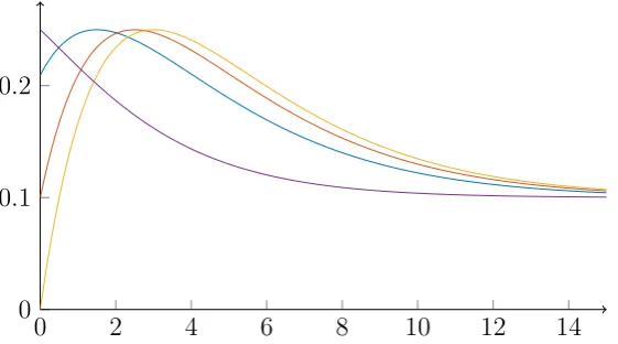
Parameterisation 2.1 The instantaneous volatility function for the Paramet-erisation 2.1 is given by the parameters α1, α2 ≥ 0, β1, β2 ∈ R, γ ∈ [−1,1] and equation (5.3). For the purpose of this discussion we will assume thatα1, α2>0 andβ_{1 6}=β₂ as the instantaneous volatility function otherwise reduces to a single exponential. Furthermore we will assume that 0 _≤ β1 < β2 to ensure that the instantaneous volatility function is bounded on_R+. Figure 1 shows plots of the instantaneous volatility function for various choices of parameter values.

Clearly this parameterisation can capture the long-term level of volatility when β1 = 0 in this case lim_x→∞σinst(x) =α1.Moreover, whenγ ∈[0,1] the functionσinst

is strictly decreasing. On the other hand ifγ _∈[₋1,0) the instantaneous volatility function has a local minimum at x0 = _β1

2 log

α1

−α2γ. Whenx

0_{≤0 the instantaneous}

0 2 4 6 8 10 12 14 0

0.1

0.2

Figure 1: Plots of instantaneous volatility as a function of time to maturity corresponding to Parameterisation 2.1 (equation (5.3)) for various different choices of parameter values.

volatility function is strictly decreasing on [0, x0) and strictly increasing on (x0,_∞). In particular whenβ1 = 0 the instantaneous volatility function cannot capture the hump, but it can capture the monotonically decreasing instantaneous volatilities and the long-term level of volatility.

Let us now consider the case when β1 > 0. In this case it is obvious that lim_x→∞σinst= 0 and the instantaneous volatility cannot capture the long-term level

of volatility. Furthermore, whenγ _≥0 it is easy to observe that the instantaneous volatility function is strictly decreasing. One can show that σinst has two local extremax0₁ and x0₂ (on_R) if and only if

γ <₋2

√

β₁β₂

β1+β2. (5.18)

In particular when γ =₋1 the local extrema occur at

x0₁ = 1 β2−β1log

α2

α1, x

0

2 = _β 1 2−β1 log

α2β2

α1β1. (5.19)

Sinceβ1< β2 it followsx₁0 < x0₂ and the local minimum is attained atx0₁ and the local maximum is attained atx0₂. Note that whenα_1≥α₂ then x0_1≤0 andσinst _is strictly increasing on (0, x0₂) and strictly decreasing towards zero on (x2,∞) and is therefore hump shaped.

To summarise, the instantaneous volatility function given by Parameterisation 2.1 cannot capture the hump and the long-term level simultaneously. However, it can capture monotonically decreasing volatilities together with the long-term level of volatility.

Parameterisation 2.2 Next we analyse the instantaneous volatility function corresponding to Parameterisation 2.2 given in equation (5.6). Figure 2 shows plots of the instantaneous volatility function for various choices of parameter values.

First observe that σinst will be bounded (onR+) if and only ifλ >0, which we will assume throughout the analysis. In this case it is clear that limx→∞σinst(x) = 0

and the instantaneous volatility function cannot capture the long-term level of volatility.

0 2 4 6 8 10 12 14 0

0.1

0.2

Figure 2: Plots of instantaneous volatility as a function of time to maturity corresponding to Parameterisation 2.2 (equation (5.6)) for various different choices of parameter values.

volatility function and one can think of β and γ as a shfit along x and y axis respectively. Note however that the shift will be non-linear and affected by the decay, i.e. the effect of varyingβ andγ on the instantaneous volatility will decrease as time to maturity increases.

It is then easy to observe that σinst has local extrema (onR) if and only if

γ < 1

4λ2, (5.20)

which is in practice a relatively mild constraint. The local extrema are then attained at

x0₁ =β+1−

p

1₋4γλ2

2λ , x

0

2 =β+1 +

p

1₋4γλ2

2λ . (5.21)

In particular,x0₁ is a local minimum andx0₂ is a local maximum.3 Note thatx0₁< x0₂ and that changing the parameterβ will shift the location of the local extrema, which is in line with the intuitive interpretation of the parameter β. Whenx0_{1 ≤}0< x0₂ the instantaneous volatility function is strictly increasing on (0, x0₂) and strictly decreasing on (x0₂,∞) and can therefore capture the hump. Furthermore, when x0_{2 ≤}0 the instantaneous volatility function is strictly decreasing on R+. Note that in both cases β <0.

To summarise, Parameterisation 2.2 can represent both monotonically decreasing and hump shaped volatilities. However it cannot capture the long-term level of volatility.

Three Factors

We have seen that the two-factor parameterisations cannot capture the hump and the long-term level of volatility simultaneously. We will show that introducing the third factor leads to significantly more flexible instantaneous volatility parameterisations, given by equations (5.11), (5.13) and (5.15), that can capture the hump and the long-term level of volatility simultaneously.

Parameterisation 3.1. First we consider the instantaneous volatility function given by equation (5.11). Figure 3 shows plots of the volatility function for various choices of parameter values.

3_Whenγ= 1

Note that, by setting α3 = 0 the instantaneous volatility function reduces to the one we get in Parameterisation 2.1. Therefore we can assume thatα1, α2, α3 >0. Furthermore, in order for the instantaneous volatility function to be bounded we will additionally require β1, β2, β3 ≥0.

0 2 4 6 8 10 12 14

0 0.1

0.2

Figure 3: Plots of instantaneous volatility as a function of time to maturity corresponding to Parameterisation 3.1 (equation (5.11)) for various different choices of parameter values.

Recall that the main weakness of the Parameterisation 2.1 is its inability to capture the hump and the long-term level of volatility simultaneously. We will therefore only concentrate on the case when β₃ = 0 andβ_{1 6}=β₂. In this case we can interpret the parameterα3 as the long-term level of volatility.

For the Parameterisation 3.1 to be valid, the matrix value functionρ(t) describing the time tcorrelation structure of the Brownian motion driving the model needs to be a correlation matrix. In the case of Parameterisation 3.1 ρ is given by

ρ(t) =



 

1 γ1,2 γ1,3 γ₁,2 1 γ2,3 γ1,3 γ3,3 1





 (5.22)

and is a correlation matrix if and only if γ1,2, γ1,3, γ2,3 ∈[−1,1] and

detρ(t) = 1₋(γ₁2_,2+γ₁2_,3+γ₂2_,3) + 2γ1,2γ1,3γ2,3≥0. (5.23)

When the third factor is independent of the first two (i.e. γ1,3 = γ2,3 = 0), equa-tion (5.23) is satisfied for anyγ1,2 ∈[−1,1] and σinst has local extrema (onR) if and only if

γ1,2 <−2

√

β1β2

β1+β2. (5.24)

Note, that this is essentially the same condition as in the Parameterisation 2.1. Moreover, it is easy to verify that the local extrema are attained at the same points as for the Parameterisation 2.1.

When the third factor is correlated with the first two, one cannot in general explicitly find the local extrema, due to the first derivative being highly non-linear. However, allowing the third factor to be correlated with the first two clearly introduces additional flexibility to the instantaneous volatility parameterisation. In particular, this flexibility is necessary when the implied volatilities of caplets with short times to maturity are below the long-term level of volatility.

main downside is that it becomes less intuitive (but remains analytically tractable) when the factor representing the long-term level of volatility is correlated with the other two factors.

Parameterisation 3.2. The instantaneous volatility Parameterisation 3.2 given by equation (5.13) is perhaps the most interesting parameterisation we can achieve in a three-factor separable and time-homogeneous model. Figure 4 shows the plots of the volatility function for various choices of parameter values.

0 2 4 6 8 10 12 14

0 0.1

0.2

Figure 4: Plots of instantaneous volatility as a function of time to maturity corresponding to Parameterisation 3.2 (equation (5.13)) for various different choices of parameter values.

Note that setting the parameter δ = 0 reduces the instantaneous volatility function to the one obtained in Parameterisation 2.1. In particular, we noted that the main drawback of Parameterisation 2.1 is its inability to capture the long term level of volatility.

Parameterisation 3.2 can capture the long-term level of volatility simply by settingµ= 0 in which case δ can be interpreted as the long-term level of volatility. In particular, by settingα=_|b|,β =₋a_b, γ = 0,δ =d, ε=₋a_b,η = sgnbandλ=c the volatility function corresponds to the Rebonato’sabcd instantaneous volatility parameterisation given by equation (2.10). In particular, the Parameterisation 3.2 can capture both hump and long term-level of volatility.

Clearly, we can get extra flexibility by also varying the parameters γ, η, however it is often sensible to set ε=β as its effect on the volatility function is relatively limited.

Parameterisation 3.3. Finally let us briefly discuss the instantaneous volatility function given by equation (5.15) corresponding to Parameterisation 3.3. Recall that the main reason for considering the three-factor models was the inability of the two-factor parameterisations to capture the hump and the long-term level of volatility simultaneously. However, note that Parameterisation 3.3 cannot capture the long-term level of volatility. Therefore it will in most case perform only marginally better over the Parameterisation 2.1 and 2.2 which does not justify the increase in the number of factors used.

5.2

Instantaneous Correlation

parameterisa-tions, which can be represented by a function ρinst :R2+→[₋1,1] whereρinst(x, y) is the instantaneous correlation between two forward rates with times to maturityx and y respectively.

Ideally one would take a similar approach as for instantaneous volatilities and determine the desirable properties of instantaneous correlations by relating them to prices of European swaptions. However, this turns out to be a difficult task as in general one cannot separate the effects of the instantaneous correlations from the effects of instantaneous volatilities on the European swaption prices (see Section 7.1 in Rebonato (2002)).

One therefore needs to take a different route and estimate the instantaneous correlations from historical data (see Section 7.2 in Rebonato (2002) and Section 14.3 in Andersen and Piterbarg (2010)). By doing so one usually observes that the resulting instantaneous correlation matrix satisfies the following stylised facts (see Section 7.2 in Rebonato (2002), Section 23.8 in Joshi (2011))

1. Instantaneous correlations are positive

ρinst(x, y)>0; (5.25)

2. Instantaneous correlations decrease as the absolute value of the difference between the two times to maturity increases

|x₋y_|<_|x₋z_{| ⇒}ρinst(x, y)> ρinst(x, z); (5.26)

3. Instantaneous correlation between forward rates with the difference between their times to maturity increases as the time to maturity of the forward rate expiring earlier increases

x < x0 _⇒ρinst(x, x+y)< ρinst(x0, x0+y); (5.27) The most basic example of an instantaneous correlation function satisfying the first two stylised facts is theexponential instantaneous correlation function given by parameterβ >0 and equation

ρinst(x, y) = exp ₋β_|x₋y_|

, (5.28)

Note that the exponential instantaneous correlation violates the stylised fact 3. To correct for this violation one can introduce thesquare-root exponential instantaneous correlation function given by parameter β0 >0 and equation

ρinst(x, y) = exp −β0 √

x−√y

. (5.29)

Figure 5 shows plots of the exponential and square-root exponential instantaneous correlation functions. We usedβ = 0.05 to specify the exponential instantaneous correlation function and choseβ0 so that the two instantaneous correlation functions agree for the pair of forward rates with times to maturity 1 and 15 years. Observe that for both functions the correlations rapidly decrease as the difference between the times to maturity increases.

We will later observe that the instantaneous correlations in the two- and three-factor separable and time-homogeneous LMM cannot achieve such a rapid decrease in instantaneous correlations. This is not only the case for the separable LMMs but will be true for low-factor LMMs in general and is a necessary compromise one needs to make when using a low-factor LMM.

0 5 10 0

5 10 0.4

0.6

0.8

1

0 5

10 0

5 10 0.4

0.6

0.8

1

Figure 5: Plots of the exponential instantaneous correlation function (left) for β = 0.05

and the square-root exponential instantaneous correlation function (right) for β0 = 0_.2436.

between the rates with times to maturityT1, . . . , Tn. Empirical studies have shown that the first three components of such a matrix can be described as ‘level’, ‘slope’ and ‘curvature’ (see Lord and Pelsser (2007) Sections 1 and 2.2, and references within).

The Two-Factor Parameterisations

We now analyse the two-factor instantaneous correlation functions we obtained in Parameterisations 2.1 and 2.2. Note that in the two-factor case the instantaneous correlation matrix is of rank two or less and will therefore have at most two non-zero eigenvectors, which we would like to interpret as level (all elements of the same sign and approximately the same value) and slope (the elements are monotonically increasing or decreasing between the first and the last elements which are of opposite sign).

Parameterisation 2.1 We begin by considering the instantaneous correlation function given by equation (5.4). Without loss of generality we can assume that α1, α2 >0, β1 6=β2. Now recall that the parameterγ is the correlation between two components of the Brownian motions driving the separable LMM.

0 5

10 0

5 10 0.9

0.95

1

5 10 15

−0.6

−0.4

−0.2

0 0.2

λ1 λ2

In particular when γ ∈ {−1,1_} the components of the Brownian motion are perfectly (inversely) correlated. In this case the LMM is essentially a one-factor model and the forward rates are perfectly correlated. Note that when γ _{∈ {−}1,1_} the resulting LMM is essentially driven by a single factor (see Remark 2.1), however it is separable in the dimension two and cannot be represented by a one-factor separable LMM.

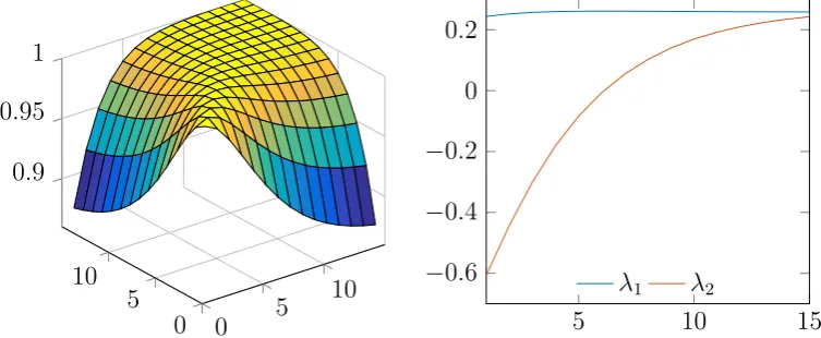
On the other hand whenγ ∈(₋1,1) the instantaneous correlation function is not identically equal to one and the resulting correlation matrix is of rank two. Moreover, the instantaneous correlations are strictly positive for every choice of parameters. However, it is in general difficult to analyse its dependence on the parameters due to complex interplay amongst them. Nevertheless, for a sensible choice of parameter values the correlation function results in mild-decorrelation between forward rates with short and long time to maturity and near perfect correlations between rates with longer times to maturity.

Figure 6 shows plots of a typical instantaneous correlation function (5.4) for a reasonable choice of parameter values and the first and second eigenvectors of the associated correlation matrix. Note that the forward rates with long maturities are nearly perfectly correlated, however there is some decorrelation between the rates of short to medium maturities and other rates. Moreover, the first two principal components of the correlation matrix can be interpreted as level and slope.

Parameterisation 2.2 We now turn our attention to the instantaneous correl-ation function given by equcorrel-ation (5.8). First observe that it only depends on the parameters β and γ.

0 5

10 0

5 10 0.8

0.9

1

5 10 15

−0.8

−0.6

−0.4

−0.2

0 0.2

0.4

λ1 λ2

Figure 7: Plot of an instantaneous correlation function (left) and the first two principal components of the associated instantaneous correlation matrix for annual forward rates with times to maturity 1 to 15 years (right) corresponding to Parameterisation 2.2.

First note that whenγ = 0 the instantaneous correlation function can be written asρinst(x1, x2) = sgn((x1−β)(x2−β)), in particular the model is effectively driven by a single factor. However when γ > 0 the instantaneous correlation function results in non-perfect correlations among forward rates.

scenario occurs when β≤0; and the instantaneous correlations are strictly positive. In this case increasingγ will decrease the correlations and decreasingβ will increase the correlations amongst forward rates.

Figure 7 shows plots of a typical instantaneous correlation function for a reas-onable choice of parameter values and the first and second principal component of a corresponding correlation matrix. Note the instantaneous correlations for rates of long-maturities are nearly perfect and there is some decorrelation between the forward rates of short and other times to maturity. Furthermore, the first two principal components can be interpreted as level and slope.

The Three-Factor Parameterisations

Having analysed the two-factor parameterisations let us now consider the three-factor Parameterisations 3.1 and 3.2. In the three-three-factor case we expect to observe curvature (the first and the last element are of the same sign but there is an element of the opposite sign which splits the elements into two monotonic sequences) in the principal component analysis of the instantaneous correlation matrix and higher levels of decorrelation.

Parameterisation 3.1 First consider the instantaneous correlation function given by equation (5.12). Recall that the matrix valued function ρ as defined in equation (5.22) is a correlation matrix describing the correlations amongst the components of driving Brownian motion. Therefore, the instantaneous correlation function will result in non-perfect instantaneous correlations only when the rank of matrixρ(t) is strictly greater than one.

0 5

10 0

5 10 0.6

0.8

1

5 10 15

−0.4

−0.2

0 0.2

0.4

λ1 λ2

Figure 8: Plot of an instantaneous correlation function (left) and the first two principal components of the associated instantaneous correlation matrix for annual forward rates with times to maturity 1 to 15 years (right) corresponding to Parameterisation 3.1 when

γ1,2 =−1.

0 5 10 0

5 10 0.6

0.8

1

5 10 15

−0.5

0 0.5

λ1 λ2 λ3

Figure 9: Plot of an instantaneous correlation function (left) and the first three principal components of the associated instantaneous correlation matrix for annual forward rates with times to maturity 1 to 15 years (right) corresponding to Parameterisation 3.1 when

γ1,2 = 0.

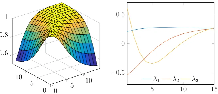
On the other hand when ρ(t) is a full rank matrix, the resulting model will be a proper three-factor LMM and the instantaneous correlation matrix will have three principal components corresponding to non-zero eigenvalues. Figure 9 shows plots of an instantaneous correlation function and the first three principal components of the associated instantaneous correlation matrix for a full rank ρ(t). Note that the principal components can be interpreted as level, slope and curvature.

Observe the correlation functions in Figures 8 and 9 have significantly different shapes demonstrating the flexibility of the instantaneous correlation function (5.14).

Parameterisation 3.2 Finally let us consider the instantaneous correlation function given by equation (5.14) corresponding to perhaps the most interesting parameterisation of the three-factor separable and time-homogeneous LMM.

We begin by noting that in the special case when the parameters are chosen so that the instantaneous volatility function corresponds to the Reobnato’s abcd parameterisation the resulting model is one-factor but it is represented by a three-factor separable parameterisation.

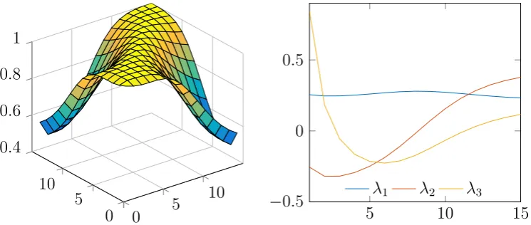
However, for a general parameterisation the instantaneous correlations will be non-perfect. Figure 10 shows plots of an instantaneous correlation function and the first three principal components of the associated correlation matrix for reasonable parameter values. Note that the instantaneous correlation function has shape similar to the one presented in Figure 8. Furthermore, observe that the principal components can be interpreted as the level, slope and curvature.

5.3

Remarks on Calibration and Implementation

Let us conclude this section by pointing out some practical remarks about the two-and three-factor separable parameterisations discussed above. Recall, that in all cases the instantaneous volatility and correlation function were determined by the same set of parameters. As a consequence, one has to simultaneously calibrate to the caplet and swaption prices.