warwick.ac.uk/lib-publications
Original citation:
Loomes, Graham and Pogrebna, Ganna. (2016) Do preference reversals disappear when we
allow for probabilistic choice? Management Science .
http://dx.doi.org/10.1287/mnsc.2015.2333
Permanent WRAP URL:
http://wrap.warwick.ac.uk/71578
Copyright and reuse:
The Warwick Research Archive Portal (WRAP) makes this work of researchers of the
University of Warwick available open access under the following conditions.
This article is made available under the Creative Commons Attribution 4.0 International
license (CC BY 4.0) and may be reused according to the conditions of the license. For more
details see:
http://creativecommons.org/licenses/by/4.0/
A note on versions:
The version presented in WRAP is the published version, or, version of record, and may be
cited as it appears here.
MANAGEMENT SCIENCE
Articles in Advance, pp. 1–20
ISSN 0025-1909 (print)ISSN 1526-5501 (online) http://dx.doi.org/10.1287/mnsc.2015.2333 © 2016 INFORMS
Do Preference Reversals Disappear When
We Allow for Probabilistic Choice?
Graham Loomes
Warwick Business School, University of Warwick, Coventry CV4 7AL, United Kingdom,[email protected]
Ganna Pogrebna
International Institute for Product and Service Innovation, Warwick Manufacturing Group, University of Warwick, Coventry CV4 7AL, United Kingdom,[email protected]
T
he “preference reversal phenomenon,” a systematic disparity between people’s valuations and choices, poses challenges for theory and policy. Using a very general formulation of probabilistic preferences, we show that the phenomenon is not mainly due to intransitive choice. We find a high degree of regularitywithinchoice tasks and alsowithinvaluation tasks, but the two types of tasks appear to evoke very different cognitive processes, even when the experimental environment tries to minimise differences. We discuss possible implications for modelling and eliciting preferences.Data, as supplemental material, are available at http://dx.doi.org/10.1287/mnsc.2015.2333.
Keywords: preference reversal phenomenon; probabilistic preferences; stochastic choice
History: Received February 13, 2015; accepted August 14, 2015, by Manel Baucells, decision analysis. Published online inArticles in Advance.
1.
Introduction
More than three decades ago, Grether and Plott (1979) drew economists’ attention to an unsettling regularity reported by experimental psychologists (Lichtenstein and Slovic 1971, Lindman 1971). The regularity in question—thepreference reversal phenomenon—took the following form. Two lotteries were constructed: a “$-bet,” which offered a relatively high payoff with a probability well below 0.5, and a “P-bet,” which offered a considerably higher probability of a more modest payoff. Participants in the experiment were asked to do three things: to place a certainty equivalent value1
upon the $-bet, to place a certainty equivalent value upon theP-bet, and to make a straight choice between the two. Most conventional decision theories suppose that an individual who prefers one bet to the other will pick the preferred option when offered a choice between the two and will also place a higher certainty equivalent value on whichever option he or she prefers.
1Most often, this value has been elicited as a “reservation selling
price”—that is, the individual is given ownership of the bet and is asked to state the smallest sure amount for which the individual would be prepared to sell the right to play out the bet. Sometimes the task is framed in terms of the maximum sure sum the individual would be prepared to pay to buy the right to play the bet and be paid accordingly. Lichtenstein and Slovic (1971) report experiments using both selling values and buying values. Luce (2000, Chapters 6 and 7) provides a detailed theoretical discussion of buying and selling prices for risky lotteries, together with some observations about the practical difficulties of eliciting such values.
However, Lichtenstein and Slovic (1971) reported that a substantial proportion of their experimental partici-pants flouted this expectation by choosing theP-bet while placing a strictly higher value on the $-bet. The opposite “anomaly”—choosing the $-bet while placing a higher value on the P-bet—was rarely observed. It is this asymmetry that constitutes the classic preference reversal (PR) pattern.
Grether and Plott (1979) had initially supposed that this phenomenon would disappear—or at least, be greatly attenuated—if stronger incentives and stricter experimental controls were deployed. But, in fact, the phenomenon persisted, and many other experiments since that time have found this classic PR pattern of behaviour to be easy to replicate and quite difficult to eliminate without considerable effort and/or supple-mentary mechanisms; see the survey by Seidl (2002).
At the level of modelling, this phenomenon would appear to present a fundamental challenge to general theories that assume transitivity. At the level of practical application, it raises concerns about the use of stated values as a basis for guiding public policy: if such patterns also occur in the domain of, say, environmental goods, there is a danger that using stated willingness to pay in cost–benefit analysis might lead to priority being given to projects that would not be chosen if citizens were in a position to express choices or rankings directly. For reasons of both theory and policy, therefore, it is important to gain a better understanding of what this phenomenon really represents in terms of
1
the structure of human preferences and/or the validity of different procedures for eliciting those preferences. This paper aims to contribute to a better understand-ing of those issues. The next section discusses in more detail the main competing explanations of PR and some of the evidence for and against the different accounts. That discussion raises issues about the noisiness or imprecision of many people’s responses, so in §3we outline a (deliberately broad) framework of probabilistic preferences within which our inquiry will be conducted. In §4 we report two substantial experiments. The data generated by these experiments strongly suggest that for pairs of bets typical of the PR literature, most people’s preferences exhibit some degree of stochastic variability, but their “core” preferences mostly conform with the probabilistic formulation of transitivity known as weak stochastic transitivity. Put another way, when certainty equivalent values are inferred from repeated binary choices, the classic PR phenomenon largely disappears, and the reversals that remain are relatively few in number and small in magnitude. By contrast, when certainty equivalent values are elicited more directly via a standard incentive-compatible mecha-nism, the same individuals display a very strong PR pattern of the usual kind. Our results broadly support the conclusions drawn by Tversky et al. (1990) and Bostic et al. (1990), although we find “overvaluation” of all bets rather than the mix of overvaluation and undervaluation that those studies report.
It is not possible to reconcile the data with conven-tional deterministic models—even those that permit some level of preference reversal (e.g., Loomes and Sugden1983). So in §5we explore the data we have generated to see whether we can shed further light on the disparities between choice and valuation, and we discuss whether we can account for them in terms of a model of probabilistic choice known as decision field theory (Busemeyer and Townsend1993). It turns out that this model—at least, as applied by Johnson and Busemeyer (2005)—cannot adequately accommodate our data, so in the final section we discuss some possi-ble directions for future theoretical development and some implications for applied research.
2.
Different Possible Explanations of
the Classic PR Pattern
Attempts to account for the PR phenomenon fall into three main categories, each of which we outline in the subsections below.
2.1. Intransitive Preferences
One possible hypothesis is that the classic PR pattern reflects preferences that allow systematic intransitivity over binary choices. Let us write the $-bet as $, write the
P-bet asP, and denote strict preference by. Suppose
we can find some sure amount of moneyM such that an individual has the preferences $M,MP, and
P$: that is, suppose that for this particular8$1 P 1 M9
triple, she has intransitive preferences.
If asked to give her certainty equivalent for the $-bet, CE($), she will state some CE($)> M; if asked to give her certainty equivalent for theP-bet, she will state CE4P 5 < M. Hence, when asked to give the two valuations and also make a direct choice between $ andP, as in standard PR experiments, she will report CE($)>CE(P) and P$, thereby exhibiting the classic PR pattern. In so doing, there is no bias or error in her responses; she is accurately reporting her preferences but happens to have preferences that, in this case, do not conform with transitivity. Although many decision theories take transitivity as axiomatic, not all theories do so; for example, regret theory (Bell1982; Loomes and Sugden1982,1983) allows preferences of the kind that would produce the classic PR pattern for at least some8$1 P 9pairs.2
Of course, if this intransitivity explanation is correct, it should be possible to find evidence of the $M,
M P, and P $ cycles that would underpin the classic PR pattern. A paper by Loomes et al. (1991) reported an experiment where choice cycles in this classic direction did indeed outnumber those in the opposite direction, seemingly to a significant extent. However, only a minority of all responses were cyclical, and it was suggested by Sopher and Gigliotti (1993) that the patterns reported by Loomes et al. (1991) could possibly have arisen purely as a result of noise/error. This is an issue to which we shall return in §2.3and §3.
2.2. Procedural Biases
A rather different kind of explanation of the PR phe-nomenon was offered by Lichtenstein and Slovic (1971). Other variants have been suggested since, but what they have in common is the idea that people may not have highly articulated underlying preferences that are always accurately and consistently expressed in response to every task, but rather may to some extent construct their responses according to the nature of the task presented to them and may therefore be systematically influenced by certain features of the different procedures used.
2An intuitive explanation of how regret theory works in this context
is as follows. An individual who behaves according to regret theory gives disproportionate weight to larger payoff differences within binary comparisons and is especially averse to being on the downside of such differences. In a8$1 M9pair, the bigger difference is between the $-bet’s high payoff and the relatively modest sure sum offered by
M, and this works againstMand favours choosing $. By contrast, in the8P 1 M9pair, the higher payoff offered byPis typically not much better than the sure sum, whereas the more influential difference is between the sure sum andP’s lower payoff, which works againstP
and favoursM. Hence we may see $MandMPeven when
P$ in a direct comparison between those bets.
So, for example, when asked to give a certainty equivalent—that is, when asked to give a response in terms of a sum of money—it may be that individuals are (subconsciously) prompted to pay extra attention to the money dimension and underweight the proba-bility information. Perhaps, especially when the task is framed as selling, they initially “anchor” on the bet’s most desirable payoff and then arrive at their valuation by adjusting down from that payoff to allow for the possibility that some lower payoff may result; but they do not adjust sufficiently and hence tend to generate a higher certainty equivalent for the bet with the higher payoff, the $-bet. By contrast, when asked to make a straight choice between $ andP, it may be that more attention is paid to the chances of winning at least something; since theP-bet offers a greater chance of winning something than the $-bet, this serves to increase the likelihood that theP-bet will be chosen. In short, the weight given to different dimensions may be influenced by the nature of the elicitation procedure, resulting in a systematic disparity between the preference inferred from direct choice and the preference inferred from the two separate valuations.
Tversky et al. (1990) conducted some experiments intended to try to diagnose the causes of preference reversals, both for risky options and for intertemporal decisions. With respect to $-bets andP-bets (which they relabelledLand H, respectively), they concluded that the phenomenon was primarily due to what they regarded as overvaluing theL4$5 bet, and was partly due to undervaluing theH4P 5bet, with perhaps 5%–10% of the effect caused by intransitivity.
However, there are reasons to be cautious about the basis for this diagnosis. One reservation concerns the mechanism used to elicit the values of the bets. Participants were told that at the end of any session involving real payoffs, a pair of lotteries would be selected at random. There was then a 50% chance that a participant would be paid on the basis of playing out whichever option he had picked in the direct choice task, and there was a 50% chance that he would instead play out whichever option he had placed a higher value upon. Whereas Tversky et al. (1990, p. 207) argued that this “ordinal payoff scheme” avoided some of the objections that had been made against the standard Becker-DeGroot-Marschak mechanism (Becker et al.
1964), it had the disadvantage that it was no longer necessary to identify the true indifference value for each bet, since it was only the ordering of the values rather than their precise magnitudes that mattered. In the absence of a mechanism designed to give accurate magnitudes, it is arguably unsafe to make statements about “overvaluing” or “undervaluing” on the basis of ordinalresponses.
Moreover, the extent to which one can detect intran-sitivity depends on whether the parameters selected by the experimenters happen to fall within a participant’s “critical” region (since regret theory, for example, does not entail preferences that areeverywhereintransitive but only allows that they may be intransitive over some range). Therefore, an experiment that uses a small set of options involving a limited number of preset parameters may well hit upon the critical region forsomeindividuals but might miss it for others with different underlying preferences, even though these peo-ple might display intransitivity in other (unexplored) triples.
The studies conducted by Bostic et al. (1990) tried to address the latter issue by eliciting choices via two different iterative procedures (while using the Becker-DeGroot-Marschak (1964) mechanism to incen-tivise valuations elicited in a more conventional way). Bostic et al. (1990) found that their first iterative choice experiment reduced the prevalence of cycles compared with classic PR patterns but did not eliminate the asymmetries between cycles for two8$1 P 9pairs out of four. Their second experiment, using a more concealed iterative choice procedure,3 seemed to reduce the
sig-nificance of asymmetrical cycles even further but had a rather small sample of just 21 respondents.
2.3. Imprecise or Probabilistic Preferences
There is a third kind of explanation that focuses on the possible importance of the impreciseorprobabilistic nature of many people’s preferences.
At the less structured end of the spectrum of such accounts, MacCrimmon and Smith (1986) suggested that the classic PR pattern could be explained in terms of the $-bet allowing a much wider range of valuation responses that do not violate first-order stochastic dominance than the range allowed by theP-bet, so that individuals who were unsure about their precise certainty equivalent could more easily pick higher values for the $-bet than for theP-bet without being obviously wrong. If both bets have (roughly) the same minimum payoff (small negative amounts in the early experiments, often zero in more recent experiments), there is more scope for giving higher values for the $-bet than for theP-bet but less scope for giving lower values, which would be sufficient to produce the classic asymmetry.
3Bostic et al. (1990, p. 204) expressed some concern that in their first
experiment, the iterative procedure may have become so transparent that it affected respondents’ answers by putting them into a valuation frame of mind. Experimental economists might also fear that a transparent procedure could encourage strategic answers intended to influence the options offered subsequently. The second procedure used by Bostic et al. (1990) was less transparent and therefore less vulnerable to those concerns.
MacCrimmon and Smith (1986) noted that if the same reasoning were applied to the elicitation of prob-ability equivalents, the opposite asymmetry might be expected.4 Butler and Loomes (2007) conducted an
experiment to explore these possibilities and found some evidence that people’s uncertainty about their own preferences varied in ways consistent with Mac-Crimmon and Smith’s conjectures.
At the more structured end of the spectrum, Blavatskyy (2009) proposed a model that embeds a deterministic expected utility theory (EUT) core in a particular stochastic specification and has shown howsomeasymmetry in the classic PR direction might result. The detail of this approach is different from that used by Sopher and Gigliotti (1993) mentioned above, but the general proposition is similar: namely, that if an individual’s expressed preferences involve some stochastic component, that component, although itself random, may interact with core preferences in such a way as to produce seemingly systematic departures from standard presumptions. Under certain conditions, this model can even accommodate what Fishburn (1988, pp. 45–46) called “strong” reversals.5
Johnson and Busemeyer (2005) explored the possibil-ity that Busemeyer and Townsend’s (1993) decision field theory might provide an explanation. The key idea is that individuals arrive at a valuation response after a cognitive process of iteration between each bet and some sequence of sure amounts. They hypothe-sised that the starting point of such a process typically involved higher sure amounts when $-bets were being valued than whenP-bets were being processed and that it was this that tended to produce CE($)>CE(P) even whenP$ in a direct comparison.
In §5, we will discuss this and the various other possible explanations outlined above. First, however, we set the scene for our experiments.
4Instead of asking for a sure amount of money that the individual
considers exactly as desirable as a particular bet, these questions ask the individual to state the probability of an even higher payoff that is regarded as equivalent to a particular bet. For example, if theP-bet were a 0.7 chance of £15 and a 0.3 chance of 0, an individual might be asked what probabilitypof £60 (with a 1-pchance of 0) would be exactly as desirable as thatP-bet; that individual might also be asked what probabilityqof £60 (otherwise 0) would be exactly as desirable as a $-bet offering a 0.3 chance of £40. Sincepcould be anywhere in the range between 0 and 0.7 without violating dominance, whereasq
is constrained by dominance to lie between 0 and 0.3, there is more scope to give a higher probability equivalent for theP-bet while perhaps choosing the $-bet in the direct choice between the two.
5A strong reversal is a case where theP-bet is chosen even though
the stated certainty equivalent for the $-bet is strictly higher than the maximum payoff offered by theP-bet. Thus, it amounts to an implicit violation of first-order stochastic dominance. Even though regret theory allows “standard” reversals, it cannot accommodate strong reversals.
3.
A Broad Probabilistic Choice
Framework
It has often been observed that when the same individ-ual is presented with exactly the same tasks framed in exactly the same way on more than one occasion within a fairly short period of time, the individual may answer somewhat differently in at least some of those repetitions. An early manifestation of such behaviour was reported by Mosteller and Nogee (1951), who encountered variability of this kind when they presented respondents with a variety of choices, each repeated multiple times over a period of several weeks. For example, one series of decisions asked respondents either to accept or refuse a gamble that involved a 1 3
chance of losing 5 cents and a 23 chance of winning
X, where X took a number of different values rang-ing from 5 cents to 16 cents. Over the course of the experiment, each level of X was presented to each respondent on up to 14 independent occasions. Figure 2 of Mosteller and Nogee (1951) depicted a respondent who never accepted the gamble whenX was 5 cents or 7 cents and always played it whenX was 16 cents, but for intermediate values, his acceptance rate lay between 7% and 93%, increasing monotonically withX. Such variability (although often less neatly monotonic) was typical of the other participants in their study and has been observed in many subsequent studies involving repeated choices.
Over the years, such variability has been formally modelled in a number of ways; see Luce and Suppes (1965) for an early review and Rieskamp et al. (2006) for a more recent one. However, as Stott (2006) and Blavatskyy and Pogrebna (2010) have shown, different assumptions about the way in which the stochastic com-ponent is specified can produce quite different estimates of underlying parameters. To avoid becoming embroiled in debates about the sensitivity of our results to particular functional forms, our strategy in this paper is to try to investigate the issues raised above within a framework of probabilistic choice so general that it encompasses a very broad range of more specific stochastic models and relies on a bare minimum of assumptions.
Consider a case where an individual is presented with a number of choices between some lotteryBand a series of increasing sure amounts denoted byAj. If these choices could be presented on a number of different occasions and under circumstances where an individual makes each choice independently of every other one— in the sense of not remembering previous choices and therefore making each new choice afresh—then we might model an individual’s underlying preferences as a probability distribution.
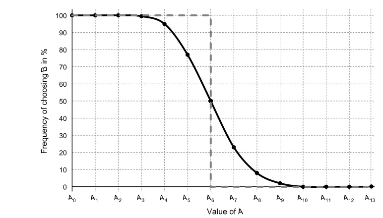
Figure 1 shows two possible distributions. The dashed line shows the deterministic preferences of an individual who is indifferent betweenB and a sure amountA6: for allj <6, she always choosesB; for all
Figure 1 Deterministic and Probabilistic Preferences
0 10 20 30 40 50 60 70 80 90 100
Frequency of choosing
B
in %
Value of A
A0 A1 A2 A3 A4 A5 A6 A7 A8 A9 A10 A11 A12 A13
j >6, she never choosesB; and for j=6, all probability mixes ofAandBare equally good.
The solid curve shows the underlying distribution for an individual with probabilistic preferences. In this example, when the sure thing is less than or equal toA3,
the individual always choosesB; when the sure thing is equal to or greater thanA10, he never choosesB. But for
values ofAbetweenA3 andA10, there is some chance that eitherAorB might be chosen. For example, when presented with a choice betweenBandA5, there is a 0.77 chance he will chooseB; therefore, if he made that choice 100 times on separate and independent occasions, we would expect on average to observe him choosing the sure amount on 23 of those occasions. Increasing the sure amount toA8increases the likelihood that the sure
sum will be chosen—to 0.93—but in 100 repetitions of the choice we would still expectBto be chosen on average on seven occasions.
Using Pr4AB5to denote the probability of choosing
Afrom the pair8A1 B9, we shall refer to cases where Pr4AB5=Pr4BA5=005 as cases of stochastic indif-ference(SI). This is the stochastic analogue of the notion of certainty equivalence in deterministic theories. In the example shown in Figure1, the SI point is atA6.
The curve in Figure1is no more than an illustration, and we make no strong claims about its shape. We have drawn it as sigmoid because that seems to fit many intuitions and data sets. We leave open the question of symmetry. Some model specifications may imply symmetry, whereas others may suggest particular kinds of asymmetry; however, such detail is not necessary for our purposes. All we wish to convey in Figure1is the distinction between deterministic and probabilistic choice and the broad proposition that models of proba-bilistic choice allow there to be some range between the
point whereB is always chosen and the point whereB
is never chosen,6and that between those two points
the probability of choosingB falls monotonically asA
is unambiguously improved.
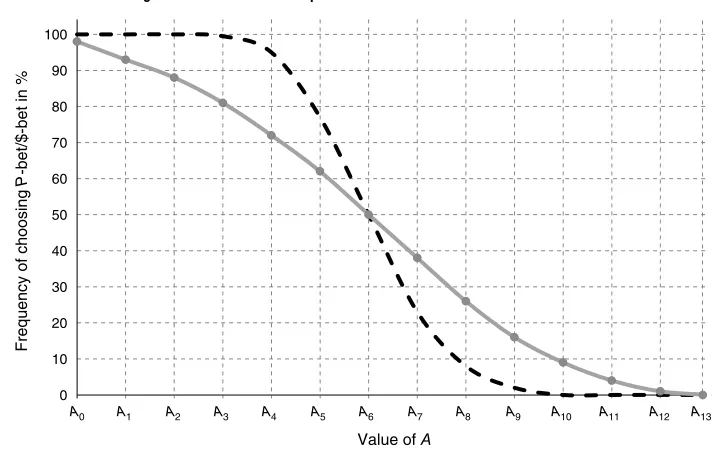
Now let us consider two different lotteries rep-resented on the same diagram. In Figure 2, let the dashed curve represent the distribution for a particular
P-bet, and let the solid curve represent the distribution for a particular $-bet, where Pr4$P 5=Pr4P$5=
005 and where both of these bets are stochastically indifferent to the sure amount A6. Thus, we have
constructed a case that is consistent with weak stochas-tic transitivity (WST), which, for any triple8X1 Y 1 Z9, requires that if Pr4XY 5≥005 and Pr4Y Z5≥005, then Pr4XZ5≥005.
However, even when WST holds, patterns of choice over specific pairs located away from the SI points may exhibit what looks like systematic disparities. To see this, suppose that we have a sample of 100 individuals whose preferences are each as in Figure2. Instead of asking them to choose between pairs involving A6,
suppose we set the sure amount at A8.
Each participant is assumed to make each choice as if on the basis of independent draws from the underlying distributions in Figure2. Most will give responses that are consistent with transitive orderings over8$1 P 1 A89, but there will be some sets of choices
6Here, we are abstracting from what have come to be called
“trembles”—that is, cases where a transparently inferior option is chosen, perhaps because of some lapse of attention. For example, in cases where one option transparently dominates the other, it has been observed that the dominated alternative is chosen in a small proportion of cases—typically 1%–2%. Our figures, here and later, omit such trembles.
Figure 2 Two Different Lotteries Having the Same SI When Compared withA
Value of A
A0 A1 A2 A3 A4 A5 A6 A7 A8 A9 A10 A11 A12 A13 0
10 20 30 40 50 60 70 80 90 100
Frequency of choosing
P
-bet/$-bet in %
that are intransitive, either in the direction consistent with the classic PR or in the opposite direction.
The cycle corresponding with the classic PR pattern is $A8,A8P, and P$. From Figure2we read
off Pr4$A85=0027 and Pr4A8P 5=0093. Combining
these probabilities with Pr4P$5=005 and assuming independent draws, the product of these probabilities is 0.12555, so that on average we should expect to observe 12 or 13 members of our sample exhibiting the cycle consistent with the classic PR pattern. The opposite cycle involves $P,P A8, andA8$, for which
the probabilities are 0.5, 0.07, and 0.73, respectively, giving a product of 0.02555, so that we should expect two or three people to report this pattern. Even if we round the first number down and round the second number up, we have a 12:3 ratio between the two cycles. If we were to apply the standard binomial test, in effect, testing the null hypothesis that both types of cycles are equally likely, we should reject that hypothesis at the 5% level. Thus, we can see how probabilistic preferences, which respect transitivity at the core, may nevertheless give theappearance of systematic asymmetries in responses to a particular set of predetermined options.
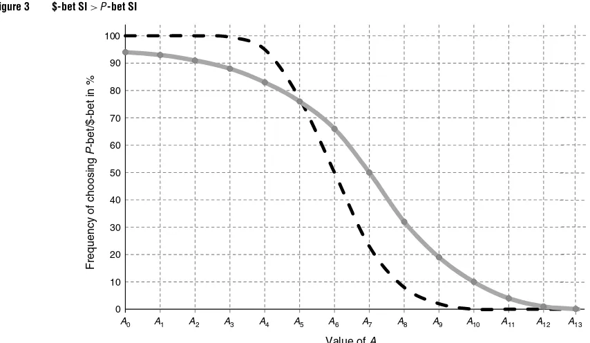
How might we depict probabilistic preferences that donot respect WST? Suppose we could find a8$1 P 9
pair such that Pr4P$5 >005 while at the same time the underlying probability distributions for each bet against different sure sums is as in Figure3.
As in Figure 2, the dashed curve represents the
8Aj1 P 9relationship, and the solid curve shows8Aj1$9. Here, the SI for the $-bet is A7, whereas the SI for
theP-bet is A6. So if we set the sure sum between
A6 and A7—halfway between, for example, which
we denote byA∗—then we should see WST violated
because at that level of A, Pr4$A∗5=0058 while
Pr4A∗P 5=0065, which should imply Pr4$P 5≥005,
whereas we have a8$1 P 9pair such that Pr4$P 5 <005. Notice, however, that such a violation of WST is only observable forAj between A6andA7. If we were to set the sure sum at anything less than A6, both
Pr4$Aj5and Pr4PAj5 >005, so that no violation of WST can be detected and likewise when the sure sum is greater thanA7 so that both of those probabilities are less than 0.5. Even if underlying preferences are as shown in Figure 3, the scope for demonstrating violations of WST in the direction consistent with the classic PR pattern is limited. It is easy to see that even if all individuals have preferences with the potential to violate WST, they may have different SIs such that any particular preset value of Awill only fall into the critical range for a subset of them.
So if we wish to provide a comprehensive examina-tion of the extent to which probabilistic preferences respect WST for $- andP-bets, we need to elicit from each individualsome estimate of his or her SI for each lottery against some set of sure amounts and see how the ordering of these SIs compares with the modal choice between them. Denoting the SI for theS-bet as SI($) and the SI for the P-bet as SI(P), the possibili-ties are as follows. If SI4P 5≥SI($) and Pr4P$5≥005, or if SI($)≥SI4P 5and Pr4$P 5≥005, the individual conforms with WST. However, if SI($)>SI4P 5 but Pr4P $5 >005, the individual violates WST in the direction consistent with the classic PR pattern, whereas if SI4P 5 >SI($) but Pr4$P 5 >005, the violation of WST is in the opposite direction. The experimental design
Figure 3 $-bet SI> P-bet SI
0 10 20 30 40 50 60 70 80 90 100
Frequency of choosing
P
-bet/$-bet in %
Value of A
A0 A1 A2 A3 A4 A5 A6 A7 A8 A9 A10 A11 A12 A13
described in §4seeks to obtain the required estimates of SI($), SI4P 5, and Pr4$P 5.
4.
Experimental Design
4.1. General Principles
In principle, we should like to take various $-bets and
P-bets and, for each bet, identify the range of sure sums that cover the distance between the highest sure sum, which is (almost) never preferred to the bet, and the lowest sure sum, which is (almost) always preferred to the bet. Within that range, we would like to have identified enough pairs, each repeated enough times (ideally, with each choice independent of all earlier presentations of the same pair) to provide a good estimate of the curve in question and a reasonably precise estimate of the SI point.
Bearing in mind that any sample is likely to involve some degree of heterogeneity between individuals, in an ideal world one might like to have different sure sums £0.50 or £1 apart covering most of the range between the upper and lower P-bet payoffs, with perhaps 10 repetitions of each8Aj1$9and8Aj1 P 9 pair. One might also like to have comparable numbers of repetitions between each8$1 P 9pair. However, such a design could easily entail four or five hundred choices for a single8$1 P 9pair, which, when interspersed among a similar number of “distractor” choices, would be a daunting prospect for potential participants and might compromise the quality of the data.
On the basis of our own and colleagues’ experience and a pilot study, we judged that we should produce a
design using no more than 200–300 questions in total, with a number of these questions involving tasks other than binary choices to try to provide some variety and extra interest for participants.7The net result was
a design that included up to 36 different pairs, with each pair presented as binary choices (BCs) on four occasions during the experimental session and with each of these presentations being separated from one another by a number of other pairs also presented in random order.
We shall set out in subsequent subsections the partic-ular parameters used, and we shall present evidence to demonstrate that the data showed reasonable sensitivity to variations in those parameters. But first we address a possible concern about whether four repetitions are sufficient for our purposes. Certainly, if our objective were to produce a reasonably tight-fitting curve for each individual for each lottery, four observations per
7When respondents are presented with a large number of tasks, there
is necessarily a judgment to be made about the balance between task load and the quality of the data generated. However, it is not possible to conduct research into within-person variability without asking several series of questions, each repeated at least several times. Inevitably, this is liable to weaken the incentive per question. One of us, Loomes (2014), has cast doubt upon the quality of the data in a study by Guo and Regenwetter (2014), which asked respondents to make 1,600 choices between pairs of lotteries in approximately 80 minutes. However, the doubts about those data are based on an analysis of evidence of low sensitivity to parameter variations and abnormally high rates of violations of transparent dominance. Our task load was much lower than that in Guo and Regenwetter (2014), and as we shall see, our data exhibited good sensitivity to parameter variations and respectable levels of within-task coherence.
Figure 4 Estimating SIs for Two Bets
0 1 2 3 4
3 4 5 6 7 8 9 10 11 12 13
Times bet is chosen
Value of $ in £
pair would not be sufficient. However, for the purpose of covering the range within which nearly everyone’s SI is located and thereby getting an estimate of each SI, we believe that our design is adequate.
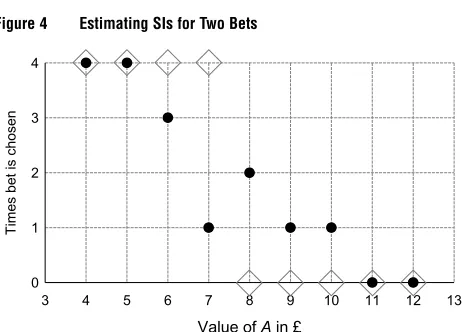
To explain how we analysed the data, consider Figure 4, which shows on the horizontal axis the different sure values thatAj might take. The vertical axis measures the numbers of times some bet is chosen in any four repeated pairings with the sameAj.
The black dots represent the responses of an indi-vidual with probabilistic preferences. When asked to choose between a $-bet and nine sure sums, each presented on four separated occasions, the individual always chooses the $-bet when the alternative is £4 or £5 and never chooses it whenAj offers £11 or £12 for sure. But for sums from £6 to £10, she chooses each alternative on at least one occasion—and is even observed to choose the $-bet more often (twice) when the sure amount is £8 than when the sure amount is £7. Of course, such seeming inconsistency is likely to occur simply by chance if the individual is behaving as if sampling just a few times from an underlying probability distribution of the kind described in §3.
The individual’s choices between aP-bet and the same set of sure amounts are shown by the grey diamonds. She always chooses theP-bet when the sure alternative is £7 or less, and she never chooses the bet when the sure sum is £8 or more. Her behaviour here is indistinguishable from what we might expect of someone with deterministic preferences whose CE lies between £7 and £8, and if we have to give a best estimate of that CE, we have no reason to do other than take the midpoint of £7.50. The same applies to our best estimate for the SI of an individual with probabilistic preferences who reports those choices.
Where does this individual’s sure-sum SI for the $-bet stand in relation to her SI for theP-bet? There is more variability in the $-bet responses, but if we had to judge which of the two bets had the greater SI in terms of sure sums, we should have to conclude on this
evidence that there is no significant difference between them: for £4, £5, £11, and £12, the same choices are made throughout; when the sure sum is £6 or £7, the
P-bet is chosen four more times; but when the sure sum is £8, £9, or £10, theP-bet is chosen four fewer times. With the small number of discrete choice observations involved, sophisticated econometric estimation may offer little more than we can achieve by simply counting the number of times each bet is chosen out of the total of 36 decisions. In the above example, each bet is chosen 16 times against the same set of sure amounts, mapping to an SI value of £7.50.
Had the individual in the above example chosen, say, the P-bet more often, it would have suggested a higher SI value for that bet. For example, suppose that she had made the same choices as above except that she had chosen theP-bet twice in the8£81 P 9 pair. On that basis, an SI of £8 would seem to be the best estimate. In other words, choosing the bet 18 times in total maps to an SI value of £8. More generally, when the range of sure options is as shown in Figure4 and when each {Aj, bet} pair is presented on four separated occasions, we estimate SI(bet)=£305+0025B, where 0< B <36 is the total number of times a particular bet is chosen.8
We shall therefore conduct our analysis of SI points in terms of the numbers of times the bet in question is chosen from any given range of alternatives. There will, of course, be some sampling error for such a measure, but our sample sizes in conjunction with the within-subject nature of the analysis will still allow us to draw a number of conclusions.
4.2. Experiment 1
Experiment 1 examined the relationship between direct choice between $ and P and the ordering of the SI values inferred from repeated choices involving the same set of sure amounts. In short, it was designed to look for evidence about conformity with—or else systematic departure from—WST when such bets are involved. The conventional wisdom, as expressed in Rieskamp et al. (2006, p. 648) is that violations of WST are quite rare and tend to occur only in “fairly unusual” circumstances, so that “the principle of weak stochastic transitivity should generally be retained as a bound of rationality.” Unfortunately, a number of the experiments they cite could be argued to have involved too few repetitions over too narrow a range to provide a really strong foundation for this conclusion. Our experiment had the drawback that it was constructed around just one8$1 P 9pair, but its strength was that
8The SI value is not well defined ifB=0 or ifB=36: in the former
case, we can only conclude that SI≤£3050 and in the latter case that SI≥12050; but for all other cases, each extra observation of the bet being chosen is counted as increasing the SI by £0.25.
Figure 5 (Color online) Examples of Displays Used in Binary Choices
(a) Binary choice between the focal $-bet and the focal P-bet
(b) Binary choice between the focal $-bet and an amount of money for certain
it involved multiple repetitions and therefore gave a reasonable chance of detecting violations of WST, if there were any to be detected.
In our pair, what we shall call thefocal$-bet offered a 0.3 chance of £40 (otherwise 0), and ourfocalP-bet offered a 0.7 chance of £15 (otherwise 0). Each bet was displayed as shown in the upper panel of Figure 5
when participants were being asked to make a straight choice between the two bets and as in the lower panel of Figure5when the alternative was a sure sum of money—in this case, the choice is between our focal $-bet and £11 for sure. The text accompanying each kind of choice is also reproduced.
We opted for this way of displaying alternatives to try to strike a compromise between the “decision by description” and “decision by experience” approaches. A growing literature9suggests that when people form
an estimate of probabilities on the basis of some sam-pling experience, they may behave differently from when the probabilities are merely described in decimal or percentage form without the opportunity for partici-pants to get some “feel” for them. The large number of decisions in our design made it impossible to ask people to learn the probabilities for each choice by sampling, but by depicting the distributions of balls
9A good selection is listed at http://dfexperience.unibas.ch/
literature.html(accessed July 5, 2015).
that give positive or zero payoffs in a format that allowed probabilities to be easily seen and compared, we hoped to provide a visual proxy for experience by showing exactly what each option would involve in terms of the 20 balls that would be put into a bag when one of the choices came to be played out for real.
The focal $-bet was presented on four separated occasions in choices with nine different sure integer amounts from £4 to £12, providing a total of 36 BCs. The focalP-bet was offered against the same nine sure sums, giving another 36 choices. We also had nine pairs where the focal $-bet was fixed while the alternative bet’s probability of £15 varied from 0.5 to 0.9 with increments of 0.05, each presented on four separated occasions; and another nine pairs where the focalP-bet was held constant while the alternative bet’s probability of £40 varied from 0.15 to 0.55 with increments of 0.05. Thus, we have a total of 4×9×4=144 BCs. For each individual, then, we can estimate a certainty equivalent SI for the focal $-bet and a certainty equivalent SI for the focal P-bet, and we can compare the ordering of these SIs with the frequency of choice from a total of eight separated presentations of the focal8$1 P 9pair.
This experiment involved 101 participants through the online recruitment system of the Decision Research at Warwick (DR@W) Group in the University of War-wick. Each participant received an invitation with detailed instructions together with a link to the online
experiment. Participants were invited to complete the online experiment in their own time by a specified deadline. Each invited participant was assigned a unique ID number, which was automatically copied as a password to the experimental interface. This ensured that (a) only invited participants could take part in the experiment, and (b) none of participants could take part more than once. The experiment was com-puterised using the Experimental Toolbox (Expert)10
online platform.11
Besides the 144 BC questions described above, there were a further 36 questions presented in the form of four nine-row choice lists; these took the total of incentivised lottery-based tasks to 180, with these being mixed up and spread over sections 1, 3, and 5 of the experiment. Sections 2 and 4 consisted of quite different tasks involving 2×6 hypothetical questions of the type used in the domain specific risk attitude (DoSpeRT) procedure (Blais and Weber2006). These two sections were included as “distractor” tasks for our participants, providing greater separation between repetitions of the incentivised questions. They play no part in our analysis.
The incentive mechanism was as follows. On the date of the specified deadline, 100 participants were selected at random from all participants who com-pleted the experiment on time.12 These participants
were invited to the DR@W experimental laboratory for individual scheduled appointments. One of the 180 incentive-linked questions was picked at random and independently for each participant and was played out for real money. There was no show-up fee, and the instructions made it clear that the participant’s entire payment depended on how her decision played out in the one randomly selected question.
If the participant had chosen some sure amount of money, she would simply receive that sum. If she had chosen a lottery, she would see an opaque bag being filled with the numbers of red and black balls (actually, coloured marbles) specified in the question. She then picked a marble at random and was paid (or not) accordingly.
10http://gvp4c7.experimentaltoolbox.com/.
11Access to the experiment can be obtained by contacting the authors. 12This experiment was, in fact, one of two being conducted in parallel
using the same general format of displays but with quite different questions. A total of 101 participants saw the questions relating to preference reversal as reported in this paper. Another 148 were presented with questions that were investigating the independence axiom—the results of which are reported in Loomes and Pogrebna (2014b). So in total, 249 individuals participated in one or other of the experiments, and the 100 who played a decision for real were drawn at random from the 249. At the time when individuals were deciding to take part, neither they nor we knew what the total number of participants would be, but the promise to pay 100 individuals seems to have been sufficiently attractive to induce a high (by DR@W standards) take-up.
This incentive mechanism was described to all partic-ipants in the instructions. Particpartic-ipants also received a practice question and had an opportunity to email the experimental team in case they were not clear about the instructions. On average, it took each participant 30–40 minutes to complete the online experiment. Each individual appointment in the DR@W laboratory lasted between three and five minutes. The average payoff in the experiment was approximately £12.
We begin by presenting various aggregate patterns of response, so that readers can form some view about the extent to which the data showed broad regularities of the kind most models might entail. Table 1shows how the likelihoods of choosing the fixed lotteries changed as the alternatives were progressively improved. In all cases, the proportions were sensitive in the expected directions to variations in parameters.
At this aggregate level, the central tendencies look broadly consistent with transitivity. Overall, theP-bet was chosen in just over 83% of the direct choices between the focal $-bet and the focal P-bet. At the same time, on the basis of the choices between each bet and the different sure amounts, the sample median valuation of P was a little over £9 and the sample median valuation of $ was £7. At this level of analysis, the majority choice was compatible with the ordering of median values.
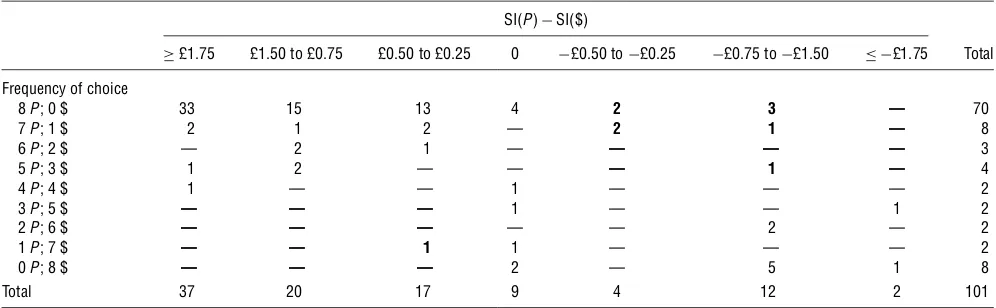
However, the usual PR asymmetry is an individual-level phenomenon. Therefore, Table 2 assigns indi-viduals to cells according to the relationship between the frequency with which they chose $ or P in the direct choice between them (shown in the rows) and the ordering over the two bets inferred from the dif-ference between their SI certainty equivalents, with the SI differences being grouped into seven column categories.
The observations that represent a strict reversal of one kind or the other are shown in bold. In total, 10 of the 101 individuals fell into these cells, with another 10 either choosing each bet equally frequently or having the same SI certainty equivalents (or both, in one case). The 10 strict reversals were divided 9:1 in the “usual” direction—an asymmetry that appears unlikely to have occurred by chance—but by comparison with most PR experiments involving direct elicitation of sell-ing/buying prices, the overall proportion of reversals was low. Moreover, the magnitudes of the differences were small by comparison with many selling price experiments—in the present experiment, the greatest SI difference in the “wrong” direction was just £1.50. So it might be argued that there was sometendency toward intransitivity in the classic direction that cannot be explained simply in terms of noise/error; but the effects were modest and the overall picture is compatible with the great majority of participants’ responses respecting weak stochastic transitivity.
Table 1 Aggregate Binary Choice Proportions in Experiment 1
Sure amounts
£4 £5 £6 £7 £8 £9 £10 £11 £12
$-betachosen % 7807 6504 6002 5000 4106 3509 1508 1506 807
P-betachosen % 9201 8704 8102 7502 6409 5302 2800 1808 1209
Chances of £15 offered by variants of theP-bet
0.5 0.55 0.6 0.65 0.7 0.75 0.8 0.85 0.9
$-betachosen % 59.9 34.9 29.5 18.3 17.6 12.6 7.2 6.4 4.2
Chances of £40 offered by variants of the $-bet
0.15 0.2 0.25 0.3 0.35 0.4 0.45 0.5 0.55
P-betachosen % 98.5 97.0 94.3 84.4 74.8 58.2 43.3 26.0 17.8 aFocal $-bet=(£40, 0.3; 0, 0.7); focalP-bet=(£15, 0.7; 0, 0.3).
However, Experiment 1 was built around just one particular8$1 P 9 pair, and it could be objected that the results might not generalise to other pairs. Moreover, Experiment 1 focused exclusively on choice-based tasks and did not at the same time elicit valuations in a more direct way, using the kind of incentive mechanism more commonly used in conjunction with selling prices in traditional preference reversal experiments. Therefore, in Experiment 2 we used slightly more extreme bets that might be regarded as (even) more typical of many PR experiments, and we added a conventional valuation task to the other formats used in Experiment 1 so that we could make direct within-person comparisons.
4.3. Experiment 2
Many features of this experiment were the same as in Experiment 1 in terms of the numbers of binary choices and the incentive system for those choices. The two key differences between this experiment and the previous one were as follows. First, the new focal $-bet offered a 0.25 chance of £50 (otherwise 0), and the new focalP-bet offered a 0.8 chance of £12—that is, the two bets were a little farther apart in terms of
Table 2 Choice and SI Valuation Differences Inferred from BCs in Experiment 1
SI4P 5−SI($)
≥£1075 £1.50 to £0.75 £0.50 to £0.25 0 −£0050 to−£0025 −£0075 to−£1050 ≤ −£1075 Total
Frequency of choice
8P; 0 $ 33 15 13 4 2 3 — 70
7P; 1 $ 2 1 2 — 2 1 — 8
6P; 2 $ — 2 1 — — — — 3
5P; 3 $ 1 2 — — — 1 — 4
4P; 4 $ 1 — — 1 — — — 2
3P; 5 $ — — — 1 — — 1 2
2P; 6 $ — — — — — 2 — 2
1P; 7 $ — — 1 1 — — — 2
0P; 8 $ — — — 2 — 5 1 8
Total 37 20 17 9 4 12 2 101
probabilities and payoffs and expected values than the pair in the first experiment. Second, we dropped the DoSpeRT questions and replaced them in sections 2 and 4 with 20 direct valuation (DV) tasks linked to the kind of incentive mechanism often used, owing to Becker et al. (1964). Those 20 DV tasks involved five different lotteries, each valued on two separated occasions in section 2 and again twice each in sec-tion 4, thus giving four separated valuasec-tions for each lottery. Figure6shows an example of a typical DV task—in this case, for the focalP-bet in the current experiment.
Two of those five lotteries were the $-bet andP-bet, which are focal to this experiment. Two others were the $-bet and P-bet used in Experiment 1. The fifth lottery was one used in the “independence” experiment run in parallel with Experiment 1, as referred to in Footnote 12.
By embedding the DV tasks among many BCs involv-ing the same or similar bets and sure amounts, our intention was to give participants every opportunity to be consistent across the two types of tasks. We also
[image:12.612.57.555.583.737.2]Figure 6 (Color online) Example of Display Used in Experiment 2 Direct Valuation
tried to formulate the valuation task to be as much like a choice task as we could, avoiding any reference to “price” or to selling or buying. That is, we were consciously attempting to reduce any framing effects so as to examine the question of whether a valuation task per se was treated differently than a series of binary choices.
To respond, participants used a mouse to click on the button—which was always initially located at zero to avoid any differential “starting point” effects between the different lotteries—and to move it along the slider. As the button moved, two values that were multiples of £0.10 and were always £0.10 apart appeared in the boxes just above the slider, rising or falling as the button was dragged right or left. Once a participant had settled on a response, he clicked on “Confirm & Proceed” and then either valued a fresh lottery or else, at the end of each series of 10 valuations, moved on to another series of BCs.
So, for example, an individual might move the slider, steadily increasing the amounts shown in the boxes until, say, the left-hand box displayed £7.50 and the right-hand box displayed £7.60. The respondent would thereby be stating that he would rather play the lottery than get £7.50 and would rather get £7.60 than play the lottery.
A total of 184 participants from the University of Warwick completed all of the BC and DV questions. On this basis, for each participant, we could identify from the BC responses
• the individual’s SI certainty equivalent for the $-bet,13
• the individual’s SI certainty equivalent for the
P-bet, and
• the distribution of eight straight choices between $ andP.
From the 20 DV questions, we had14
• four estimates of the certainty equivalent of the $-bet in this experiment,
• four estimates of the certainty equivalent of the
P-bet in this experiment,
• four estimates of the certainty equivalent of the $-bet used in Experiment 1,
• four estimates of the certainty equivalent of the
P-bet used in Experiment 1, and
• four estimates of the certainty equivalent of a lot-tery offering (£40, 0.8; 0, 0.2) used in the independence experiment for which we have BC-based SIs.
13For both bets, estimated to the nearest £0.25.
14Throughout, we took the lower of the two numbers in the boxes to
avoid any possibility that any overestimate could arise from taking the halfway point in the £0.10 difference.
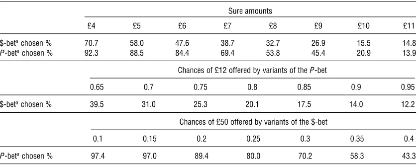
Table 3 Aggregate Binary Choice Proportions in Experiment 2
Sure amounts
£4 £5 £6 £7 £8 £9 £10 £11
$-betachosen % 70.7 58.0 47.6 38.7 32.7 26.9 15.5 14.8
P-betachosen % 92.3 88.5 84.4 69.4 53.8 45.4 20.9 13.9
Chances of £12 offered by variants of theP-bet
0.65 0.7 0.75 0.8 0.85 0.9 0.95
$-betachosen % 39.5 31.0 25.3 20.1 17.5 14.0 12.2
Chances of £50 offered by variants of the $-bet
0.1 0.15 0.2 0.25 0.3 0.35 0.4
P-betachosen % 97.4 97.0 89.4 80.0 70.2 58.3 43.3 aFocal $-bet=(£50, 0.25; 0, 0.75); focalP-bet=(£12, 0.8; 0, 0.2).
Although the last three sets of certainty equivalents do not give us the within-person information that we can get from the first two, the participants in all experiments were drawn from the same sampling frame—the DR@W list mentioned earlier—and we hoped that the additional between-sample information might prove useful.
Table3presents some aggregate results for the BC responses in the current experiment, comparable with the data presented in Table1for Experiment 1.
As before, the aggregate data look responsive in the expected direction across the different parameter variations. The sample median value for theP-bet was somewhere between £8 and £9, and the sample median value for the $-bet was below £6. In direct choices between the focal $-bet and the focal P-bet, P was chosen 80% of the time. So, as before, the aggregate data look broadly consistent with transitivity.
However, as before, the data that are most relevant for our purposes are the individual-level comparisons. Table 4displays the BC-based results for Experiment 2 in a similar format to that used in Table 2 for the previous experiment.
Again, the numbers shown in bold font highlight cases where there were strict reversals between the ordering inferred from the SIs and the majority of choices in the8$1 P 9 pairs. This time there were 13 individuals—just over 7% of the sample—exhibiting such reversals, dividing 12:1 in the direction consistent with the usual PR asymmetry. So although this asym-metry was unlikely to have occurred by chance, the overall magnitude of the effect was again rather modest and far short of the scale necessary to underpin the rates of preference reversal reported in most studies.
We now consider the DV responses generated by the same 184 individuals. Most participants’ four DVs for each bet showed some degree of variability: if we compute the standard deviation of each individual’s four DVs for each bet, there were just 16 (8.7%) who had
zero standard deviations for both bets.15The sample
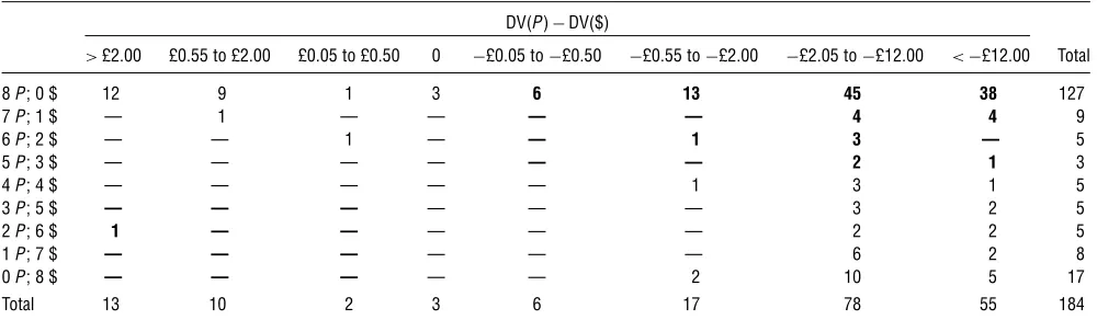
average (median) of individual standard deviations was 0.88 (0.58) for the P-bet and 4.32 (2.89) for the $-bet. Since the median DVs show less vulnerability to outliers and are comparable with SIs, Table 5replaces the SI differences in Table4by differences between the median values derived from the DV tasks. However, since individuals’ DV differences covered a much wider range than their SI differences, the column specifications are adjusted accordingly.
Clearly, the DV tasks elicited responses that were substantially different from the patterns of values inferred from BCs. Table 4shows that 46 individuals (25% of the sample) had SI($)>SI(P), whereas Table5
shows that for 156 (84.8%) individuals, median DV($) was higher than median DV(P). As a consequence, the DV tasks produced 117 classic preference reversals, compared with just one individual reversing in the opposite direction.
Going from a ratio of 12:1 BC-based reversals to a ratio of 117:1 DV-based reversals is a remarkable disparity. It is striking that 102 (87.2%) of those 117 choseP on all eight occasions when asked to make a direct 8$1 P 9 choice. It is even more striking that no fewer than 85 of these—nearly half of the sample— exhibited strong reversals of the kind referred to in Footnote 5: that is, even though their median value for the $-bet was strictly higher than the £12 payoff offered by theP-bet, they chose theP-bet over the $-bet on every one of the eight occasions when they were asked to make a straight choice. Although Blavatskyy’s (2009) model can, in principle, accommodate some strong reversals, the parameters we used lie outside the set to
15Of these, seven always stated the expected values of the bets;
one always gave a value of £10, and eight always gave extreme values−7 stating the maximum payoff for each bet, with one stating the maximum payoff for the $-bet and the minimum payoff for the
P-bet.
Table 4 Choice and SI Valuation Differences Inferred from BCs in Experiment 2
SI4P 5−SI($)
>£2000 £1.25 to £2.00 £0.25 to £1.00 0 −£0025 to−£1000 −£1025 to−£2000 <−£2000 Total
8P; 0 $ 68 20 19 11 7 2 — 127
7P; 1 $ 6 — — — 3 — — 9
6P; 2 $ 1 — 4 — — — — 5
5P; 3 $ — 1 2 — — — — 3
4P; 4 $ — — 1 2 2 — — 5
3P; 5 $ — — — — 2 3 — 5
2P; 6 $ — — — — 3 2 — 5
1P; 7 $ — — 1 — 1 2 4 8
0P; 8 $ — — — 2 4 9 2 17
Total 75 21 27 15 22 18 6 184
Table 5 Choice and Differences Between Median Direct Values in Experiment 2
DV4P 5−DV($)
>£2000 £0.55 to £2.00 £0.05 to £0.50 0 −£0005 to−£0050 −£0055 to−£2000 −£2005 to−£12000 <−£12000 Total
8P; 0 $ 12 9 1 3 6 13 45 38 127
7P; 1 $ — 1 — — — — 4 4 9
6P; 2 $ — — 1 — — 1 3 — 5
5P; 3 $ — — — — — — 2 1 3
4P; 4 $ — — — — — 1 3 1 5
3P; 5 $ — — — — — — 3 2 5
2P; 6 $ 1 — — — — — 2 2 5
1P; 7 $ — — — — — — 6 2 8
0P; 8 $ — — — — — 2 10 5 17
Total 13 10 2 3 6 17 78 55 184
which that possibility applies under the conditions he assumed—see Figure2in Blavatskyy (2009, p. 246). Such a large and pervasive disparity between BC and DV invites further analysis and discussion.
5.
Competing Explanations: Further
Exploration of the Data
On the basis of our data, we can confidently reject the proposition that the classic PR phenomenon results primarilyfrom intransitive choices. Rather, our data appear to be more in line with the Tversky et al. (1990) suggestion that the phenomenon is mainly due to a mixture of overvaluing the $-bet and/or undervaluing theP-bet.
However, as noted in §2, Tversky et al. (1990) only asked a limited range of one-off choice questions, and they elicited valuations via an ordinal scheme that could not be guaranteed to incentivise participants to give their best estimates of magnitudes of values. By contrast, we used a spectrum of repeated binary choices, and in our DV elicitation, we used an incentive mechanism of the more traditional type intended to encourage accurate revelation of actual values. Our data therefore offer opportunities to look more closely at the generality of the Tversky et al. conclusions.
Before doing so, we make a remark about the framing of the conclusions of Tversky et al. (1990). To say that a bet is “overvalued” or “undervalued” might be interpreted as suggesting that there is a “gold standard” against which such values can be judged, with the gold standard in this case presumably being the preferences revealed by binary choice. However, once we begin to think in terms of responses as being probabilistic rather than deterministic, it becomes harder to argue that one type of response reveals “true” preferences, whereas any others that produce different expressions of preference must be to some extent biased. Therefore, we are agnostic on the question of what constitutes “true” preference. However, and subject to that reservation, since most formal decision theories tend to be built on binary relations, we will take the BC responses as our reference point and use the terms “overvalued” and “undervalued” as shorthand ways of
describing DVs relative to the BC baseline.
We begin by considering the data from Experiment 2, which allowed us to make 184 comparisons between each individual’s median DV and his or her SI point for each bet. Starting with the $-bet, there were just 10 participants for whom median DV($)<SI($) and 1 for whom the two were equal. Thus, 94% of our
[image:15.612.57.557.267.413.2]sample gave a median DV($) strictly higher than the SI($) inferred from their repeated BCs. The sample mean of DV($) based on individual medians was £18.32, compared with a sample mean SI($) of £6.55, giving an average within-person difference of £11.77 between DV($) and SI($). The hypothesis of no differ-ence between the two is strongly rejected (p <00001). In this respect, our data reinforce the findings of Tversky et al. that the DV task overvalues the $-bet.
However, we do not concur with the conclusion of Tversky et al. (1990) about direct value elicitation under-valuing theP-bet. On the contrary, the DV responses in Experiment 2 also overvalued theP-bet, although to a much lesser extent. There were 57 participants for whom median DV4P 5 <SI(P), 4 for whom median DV4P 5=SI(P) and 123 for whom median DV4P 5 >SI(P). So two-thirds of the sample gave median DVs than were strictly higher than their SIs. The sample mean DV(P) based on individual medians was £8.87, whereas the sample mean SI(P) was £8.18, giving an average within-person difference of £0.69 and quite firmly rejecting the hypothesis of no difference between the two (p <0001). Still, the degree of overvaluation was much reduced: the average DV(P) was just 8.4% higher than the average SI(P), compared with the average DV($) being 2.8 times the size of the average SI($). Clearly, the fact that so many people overvalued the $-bet to a much greater extent than they overvalued theP-bet greatly outweighed many of the cases where SI4P 5 >SI($) and produced the very pronounced classic PR pattern reported in Table5and the large number of strong reversals.
Although we cannot conduct the same within-person analysis for the bets used in Experiment 1, we can undertake some between-sample comparisons to pro-vide further relevant epro-vidence.
When asked to make repeated BCs between different sure amounts and $=4£4010035, the 101 participants in Experiment 1 generated a sample mean SI($) of £7.22. This compares with a sample mean of £15.74 based on the individual median DV($) responses of the 184 participants in Experiment 2—again, more than double the SI-based figure. Not surprisingly, the null hypothesis is strongly rejected (p <00001).
ForP=4£1510075, the differences are smaller, with the sample mean of DV medians being £9.76 compared with an average SI4P 5of £8.64 from Experiment 1, so that the DV-based figure is about 12% higher. This difference registers as clearly significant (p <0001), once again suggesting that direct valuation also overvalues theP-bet relative to binary choice, albeit to a lesser extent than it overvalues the $-bet. Therefore, if we were to infer preferences from median DV responses, we should suppose $ to be preferred to P by 82% of the 184 participants in Experiment 2, whereas on the basis of the SIs in Experiment 1, $ was preferred
to P by fewer than 18% of participants. Such a large difference reinforces the suggestion of a substantial dis-parity between DV- and BC-based preference elicitation methods.
Finally, from another 81 individuals in a separate part of Experiment 1 focusing on the independence axiom, we have SI values forR=4£4010083010025, the fifth bet for which we elicited four DVs from each participant in Experiment 2. The 81 sets of BC responses give a sample mean SI4R5of £25.12, compared with a sample mean DV4R5of £29.02 based on the 184 median DVs. Here, for a bet that can also be regarded as a
P-bet, the sample mean of the median DVs is 16% higher, an overvaluation that is again significant at the 0.01 level.
To summarise so far, it seems clear that whatever process generates DV responses is a significantly differ-ent process from the one that produces BC responses. The question then is, what can our data tell us about the DV process?
We have seen (in Footnote 15) that with the exception of a small number of individuals who give extreme responses and a similarly small number who apply an expected value rule, the great majority display some variability in their set of four responses per bet. This could be regarded as compatible with DVs being produced by some internal “production” pro-cess, which may be different from the process that produces BCs but may exhibit its own within-task regularity.
As mentioned in §2.3, one way of modelling such a process has been suggested by Johnson and Busemeyer (2005), applying decision field theory to direct valuation tasks. They propose that individuals can be modelled as arriving at their value responses by means of a squen-tial value matching (SVM) process. In essence, they propose that it is as if an individual starts by compar-ing a particular lottery with some initial sure amount, then adjusts that sure amount up or down depending on whether the lottery seems clearly preferable or whether the sure amount seems clearly preferable, and repeats this internal iteration until he or she comes to a sure sum such that it is hard to identify a preference for one option or the other, at which point the pro-cess is terminated and that sure sum is stated as the value.
In an example they give, Johnson and Busemeyer (2005) take the initial value to be halfway between the two payoffs of a bet. ForP-bets this is a relatively low figure (in our Experiment 2, halfway between £12 and 0, i.e., £6), whereas for the $-bet it is much higher (in our Experiment 2, it would be £25). The stochastic nature of the process means that iterations starting low and working up—as forP-bets—are more likely to be terminated at values in the lower part of the interval where there is imprecision, whereas iterations starting