ScienceDirect
ScienceDirect
Procedia CIRP 00 (2017) 000–000
www.elsevier.com/locate/procedia
2212-8271 © 2017 The Authors. Published by Elsevier B.V.
Peer-review under responsibility of the scientific committee of the 28th CIRP Design Conference 2018.
28th CIRP Design Conference, May 2018, Nantes, France
A new methodology to analyze the functional and physical architecture of
existing products for an assembly oriented product family identification
Paul Stief *, Jean-Yves Dantan, Alain Etienne, Ali Siadat
École Nationale Supérieure d’Arts et Métiers, Arts et Métiers ParisTech, LCFC EA 4495, 4 Rue Augustin Fresnel, Metz 57078, France
* Corresponding author. Tel.: +33 3 87 37 54 30; E-mail address: [email protected]
Abstract
In today’s business environment, the trend towards more product variety and customization is unbroken. Due to this development, the need of agile and reconfigurable production systems emerged to cope with various products and product families. To design and optimize production systems as well as to choose the optimal product matches, product analysis methods are needed. Indeed, most of the known methods aim to analyze a product or one product family on the physical level. Different product families, however, may differ largely in terms of the number and nature of components. This fact impedes an efficient comparison and choice of appropriate product family combinations for the production system. A new methodology is proposed to analyze existing products in view of their functional and physical architecture. The aim is to cluster these products in new assembly oriented product families for the optimization of existing assembly lines and the creation of future reconfigurable assembly systems. Based on Datum Flow Chain, the physical structure of the products is analyzed. Functional subassemblies are identified, and a functional analysis is performed. Moreover, a hybrid functional and physical architecture graph (HyFPAG) is the output which depicts the similarity between product families by providing design support to both, production system planners and product designers. An illustrative example of a nail-clipper is used to explain the proposed methodology. An industrial case study on two product families of steering columns of thyssenkrupp Presta France is then carried out to give a first industrial evaluation of the proposed approach.
© 2017 The Authors. Published by Elsevier B.V.
Peer-review under responsibility of the scientific committee of the 28th CIRP Design Conference 2018.
Keywords:Assembly; Design method; Family identification
1. Introduction
Due to the fast development in the domain of communication and an ongoing trend of digitization and digitalization, manufacturing enterprises are facing important challenges in today’s market environments: a continuing tendency towards reduction of product development times and shortened product lifecycles. In addition, there is an increasing demand of customization, being at the same time in a global competition with competitors all over the world. This trend, which is inducing the development from macro to micro markets, results in diminished lot sizes due to augmenting product varieties (high-volume to low-volume production) [1]. To cope with this augmenting variety as well as to be able to identify possible optimization potentials in the existing production system, it is important to have a precise knowledge
of the product range and characteristics manufactured and/or assembled in this system. In this context, the main challenge in modelling and analysis is now not only to cope with single products, a limited product range or existing product families, but also to be able to analyze and to compare products to define new product families. It can be observed that classical existing product families are regrouped in function of clients or features. However, assembly oriented product families are hardly to find.
On the product family level, products differ mainly in two main characteristics: (i) the number of components and (ii) the type of components (e.g. mechanical, electrical, electronical).
Classical methodologies considering mainly single products or solitary, already existing product families analyze the product structure on a physical level (components level) which causes difficulties regarding an efficient definition and comparison of different product families. Addressing this
Procedia CIRP 75 (2018) 279–284
2212-8271 © 2018 The Authors. Published by Elsevier B.V.
Peer-review under responsibility of the Scientific Committee of the 15th CIRP Conference on Computer Aided Tolerancing - CIRP CAT 2018. 10.1016/j.procir.2018.04.023
© 2018 The Authors. Published by Elsevier B.V.
Peer-review under responsibility of the Scientific Committee of the 15th CIRP Conference on Computer Aided Tolerancing - CIRP CAT 2018.
Procedia CIRP 00 (2018) 000–000 www.elsevier.com/locate/procedia
15th CIRP Conference on Computer Aided Tolerancing – CIRP CAT 2018
Shape Error Modelling and Analysis by Conditional Simulations of
Gaussian Random Fields for Compliant Non-Ideal Sheet Metal Parts
Manoj Babu*
a, Pasquale Franciosa
a, Darek Ceglarek
aaWMG, University of Warwick, Coventry CV4 7AL, United Kingdom
∗Corresponding author. Tel.:+44-024-765-74501;E-mail address:[email protected]
Abstract
Accurate modelling of geometric and dimensional errors of sheet metal parts is crucial in designing correct GD&T and preventing unnecessary design changes during the development and launch of a new assembly process. A novel conditional simulation based methodology to probabilis-tically model and generate non-ideal sheet metal part geometric variations is developed. The methodology generates part geometric variations, which accurately emulate part fabrication process in terms of covariance of generated deviations. The methodology uses as inputs one or more of the following: measurement data of current parts, historical measurements of similar parts or FEM-based simulations. The proposed methodology emulates real processes and products accurately by generating non-ideal part representatives based on the aforementioned input data. Results provide an easy engineering interpretation to the designer. The methodology is demonstrated using automotive door hinge reinforcement.
c
2018 The Authors. Published by Elsevier B.V.
Peer-review under responsibility of the Scientific Committee of the 15th CIRP Conference on Computer Aided Tolerancing - CIRP CAT 2018.
Keywords: Non-ideal part modelling; Conditional simulation; Gaussian Process Regression; Variation simulation.
1. Introduction
Achieving zero defects in manufacturing necessitates sim-ulations that can emulate real processes and products accu-rately. Such simulations heavily rely on accurate representation of non-ideal parts, i.e.actual manufactured parts with geomet-ric and dimensional errors caused due to uncertainties in man-ufacturing processes. While some have dealt with non-ideal part generation [1–3], nonetheless the methodologies have ne-glected form tolerances which are essential for optimal toler-ance specification [4], thereby yielding limited results, since ne-glecting form tolerances can potentially lead to non-conforming assemblies [5,6].
Sheet metal parts produced by forming, often suffer from
splitting, wrinkling, shape changes due to springback and sur-face defects [7]. From an assembly perspective springback and surface defects are important; with springback being classified as a global defect, widely understood as deformations that affect
large or the entire part; and surface defects being classified as local defect, meaning deformations that affect a small/localised
region of the part.
Existing non-ideal part variation modelling methodologies considering form variation, can be classified into two main groups: (1) Morphing based, and (2) Deviation decomposition based. In morphing based methodologies, either a discrete sur-face representation such as mesh and Cloud of Points (CoP), or continuous parametric representation such as Bezier, NURBS,
are modified to generate non-ideal parts. In contrast, deviation decomposition based methodologies decompose the measure-ment data into a linear combination of orthogonal modes, and are applicable to discrete surface representations only. While morphing methodologies can handle both local deformations and global deformations, deviation decomposition techniques are global deformation modelling techniques.
A constrained deformation [8] based mesh morphing methodology was proposed in [9], the methodology while be-ing designer friendly needs the region of influence of defor-mation to be found, which is a non-trivial task. Skin model shapes [10], i.e. finite skin model representatives of non-ideal parts, based on skin model philosophy [11], is a framework to generate non-ideal parts and can be seen as belonging to both morphing and deviation decomposition methodologies. Vari-ous morphing based skin model shapes generation approaches are described in [10], and deviation decomposition based skin model shapes generation using principal component analysis is described in [12].
Existing methodologies involving skin model shapes gen-eration do not: (1) model local deviation, and (2) define ro-bust methodology to find correlation lengths. However, they require additional modelling effort to handle surface
continu-ities at edges [13].
Natural mode analysis [14] decomposes deviation data into linear combination of modes based on natural modes of vibra-tion. Geometric modal analysis (GMA) [15,16] an extension of
2212-8271 c2018 The Authors. Published by Elsevier B.V.
Peer-review under responsibility of the Scientific Committee of the 15th CIRP Conference on Computer Aided Tolerancing - CIRP CAT 2018.
Procedia CIRP 00 (2018) 000–000 www.elsevier.com/locate/procedia
15th CIRP Conference on Computer Aided Tolerancing – CIRP CAT 2018
Shape Error Modelling and Analysis by Conditional Simulations of
Gaussian Random Fields for Compliant Non-Ideal Sheet Metal Parts
Manoj Babu*
a, Pasquale Franciosa
a, Darek Ceglarek
aaWMG, University of Warwick, Coventry CV4 7AL, United Kingdom
∗Corresponding author. Tel.:+44-024-765-74501;E-mail address:[email protected]
Abstract
Accurate modelling of geometric and dimensional errors of sheet metal parts is crucial in designing correct GD&T and preventing unnecessary design changes during the development and launch of a new assembly process. A novel conditional simulation based methodology to probabilis-tically model and generate non-ideal sheet metal part geometric variations is developed. The methodology generates part geometric variations, which accurately emulate part fabrication process in terms of covariance of generated deviations. The methodology uses as inputs one or more of the following: measurement data of current parts, historical measurements of similar parts or FEM-based simulations. The proposed methodology emulates real processes and products accurately by generating non-ideal part representatives based on the aforementioned input data. Results provide an easy engineering interpretation to the designer. The methodology is demonstrated using automotive door hinge reinforcement.
c
2018 The Authors. Published by Elsevier B.V.
Peer-review under responsibility of the Scientific Committee of the 15th CIRP Conference on Computer Aided Tolerancing - CIRP CAT 2018.
Keywords: Non-ideal part modelling; Conditional simulation; Gaussian Process Regression; Variation simulation.
1. Introduction
Achieving zero defects in manufacturing necessitates sim-ulations that can emulate real processes and products accu-rately. Such simulations heavily rely on accurate representation of non-ideal parts, i.e.actual manufactured parts with geomet-ric and dimensional errors caused due to uncertainties in man-ufacturing processes. While some have dealt with non-ideal part generation [1–3], nonetheless the methodologies have ne-glected form tolerances which are essential for optimal toler-ance specification [4], thereby yielding limited results, since ne-glecting form tolerances can potentially lead to non-conforming assemblies [5,6].
Sheet metal parts produced by forming, often suffer from
splitting, wrinkling, shape changes due to springback and sur-face defects [7]. From an assembly perspective springback and surface defects are important; with springback being classified as a global defect, widely understood as deformations that affect
large or the entire part; and surface defects being classified as local defect, meaning deformations that affect a small/localised
region of the part.
Existing non-ideal part variation modelling methodologies considering form variation, can be classified into two main groups: (1) Morphing based, and (2) Deviation decomposition based. In morphing based methodologies, either a discrete sur-face representation such as mesh and Cloud of Points (CoP), or continuous parametric representation such as Bezier, NURBS,
are modified to generate non-ideal parts. In contrast, deviation decomposition based methodologies decompose the measure-ment data into a linear combination of orthogonal modes, and are applicable to discrete surface representations only. While morphing methodologies can handle both local deformations and global deformations, deviation decomposition techniques are global deformation modelling techniques.
A constrained deformation [8] based mesh morphing methodology was proposed in [9], the methodology while be-ing designer friendly needs the region of influence of defor-mation to be found, which is a non-trivial task. Skin model shapes [10], i.e. finite skin model representatives of non-ideal parts, based on skin model philosophy [11], is a framework to generate non-ideal parts and can be seen as belonging to both morphing and deviation decomposition methodologies. Vari-ous morphing based skin model shapes generation approaches are described in [10], and deviation decomposition based skin model shapes generation using principal component analysis is described in [12].
Existing methodologies involving skin model shapes gen-eration do not: (1) model local deviation, and (2) define ro-bust methodology to find correlation lengths. However, they require additional modelling effort to handle surface
continu-ities at edges [13].
Natural mode analysis [14] decomposes deviation data into linear combination of modes based on natural modes of vibra-tion. Geometric modal analysis (GMA) [15,16] an extension of
2212-8271 c2018 The Authors. Published by Elsevier B.V.
CAD, GD&T
Non-ideal part representatives Data from
measurement or simulation
Discretised CAD (X) Find node deviation (Z) perpendicular to surface
Zf X
Model Zas a Gaussian random field, with Xas
input domain i.e.
Conditionally simulate non-ideal part instances
(Z|Z*,X) Select Key points
Cloud of Points (CoP) from measurement or
simulation
Set key points’ deviation (Z*)
Non-ideal part modelling (Section 2.1) Non-ideal part generation (Section 2.2)
Section 2.1.1 Section 2.1.2 Section 2.2.1 Section 2.2.2
Fig. 2: Graphical illustration of methodology
Non-ideal partmodelling - Section 2.1
Non-ideal part generation-Section 2.2
Input pre-processing
CAD to Mesh representation
of part
Part measurement or Physical simulation
Obtain mesh nodes deviation information
Obtain optimum model parameters that characterize deviations..
Select Key Points
Estimate deviation of entire part
Required parts generated?
End Yes No
[image:2.595.40.288.270.412.2]Set key point deviations
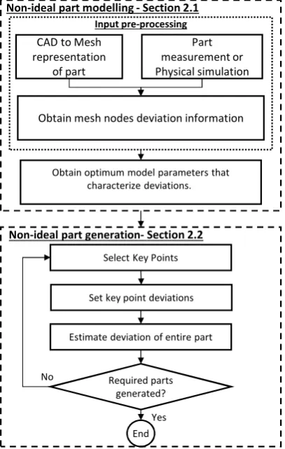
Fig. 3: Proposed non-ideal part modelling methodology
tion m(x) is defined asE[f(x)]. The covariance function be-tween two pointsxi,xj, on the surface of the part, represented
as,c(xi,xj) is defined asE[(f(xi)−m(xi))(f(xj)−m(xj))], where
Eis the expectation operator.
The mean function captures large scale trends in the devi-ation data and can be found by fitting regression models [28], or, by the maximisation of marginal likelihood as described in Section 2.1.2. In the study a zero mean function is utilised with-out affecting the analysis [25], as part variations are nominally
assumed to vary about zero mean.
The smoothness of generated deviations and the extent to which a given deviation propagates along a given direction (cor-relation length [25]), is characterised by the covariance function and its parameters. Covariance functions are classified as sta-tionary and non-stasta-tionary [22]. Areview on the types of co-variance functions with different characteristics can be found
in [25].
The choice of covariance function also affects the continuity
and differentiability of the generated non-ideal part
represen-tatives. While mean square continuity and differentiability of
the random field is easily expressed in terms of continuity of covariance function at the origin, that of generated non-ideal part instances is a complex function of covariance function as described in [24].
In the present study we choose the covariance function to characterise the GRF instead of the variogram traditionally used in geostatistics, due to the following advantages: (1) the ability to learn and model complex patterns in data with various com-binations of the covariance function [29], (2) the asymptotic properties of mean of covariance function parameters obtained in many settings through maximum likelihood estimation being equal to the true values of the parameters, and (3) the inability of the empirical semivariogram to distinguish the exact smooth-ness a differentiable process is [26].
For illustration purpose we choose the squared exponential covariance function represented by Eq. 1 where, for the three dimensional input case of non-ideal part modellingxis a 1×3 vector,σ2f is the signal variance or the scaling factor [25], and,
M is a 3×3 diagonal matrix with l−2, the inverse of square
of correlation lengths as diagonal. Representing byθthe set of all covariance function parameters{σ2f,l−2}. The aim of the
non-ideal part modelling phase is to find the optimumθthat fit the given part variation pattern, the optimised parameters are utilised during non-ideal part generation to emulate the part de-viation correlation.
c(xi,xj)=σ2fexp
−12(xi−xj)M(xi−xj)T
(1)
2.1.1. Input and pre-processing
Part variation data either in the form of physical simulation of manufacturing process (for instance from FEM analysis) or measurement of manufactured part, are utilised to obtain non-ideal part deviation from nominal. The CAD model of the part, for which non-ideal part is to be generated, is discretised to a mesh representation from which, utilising the part variation data, the deviation of each node from nominal is calculated util-ising routines in VRM software [30]. The nominal mesh node co-ordinates act as inputXto the model and surface normal de-viation of each node from the nominal, i.e. Z, is modelled as the function f(X) .
Statistical Modal Analysis (SMA) [17,18] utilises 3D-Discrete Cosine Transform (DCT) to decompose measurement data into linear combination of orthogonal modes. GMA has been ap-plied to optimise fixture design [19] and link manufacturing process parameters to part form variation [20].
In addition to the inability of above mentioned deviation de-composition based methodologies to model local part deforma-tions, the modes used in the decomposition of deviation data, usually lie in a low dimensional space, which is not easily phys-ically interpretable. Additionally, the deviation decomposition methodologies require availability of measurement data, thus, cannot be used during early design phase. A summary of capa-bilities of all discussed non-ideal part form variation modelling methodologies is presented in Table 1.
Table 1: Capabilities of part form variation modelling methodologies
Methodologies Natural mode
decomposition [14]
Geometric Modal Analysis [15,16]
Skin Model Shapes [11][13]
Morphing mesh
[9]
Proposed approach
Par
t f
or
m
var
iat
ion
m
od
el
lin
g
ca
pa
bi
lit
ie
s
Represent global
deviation
Represent local
deviation
Ensure surface continuities at
edges
Probabilistic bounds on
deviation
As afore-discussed literature shows that the existing method-ologies individually lack the ability to: 1) model simultaneously both global and local deformation, (2) ensure surface continu-ities at edges, and (3) provide easy engineering interpretation of the model parameters, and thus, are not designer friendly. In the present paper, a conditional simulation based non-ideal part modelling and generation methodology is proposed. The methodology overcomes aforementioned drawbacks and in ad-dition introduces a novel probabilistic view on deviation mod-elling. The contributions of the study are: (1) the ability to generate both local and global part deformations, (2) a de-signer friendly/intuitive form variation generation methodology
with physically meaningful model parameters, and (3) provid-ing probabilistic bounds on generated part deviations.
The rest of the paper is organised as follows; Section 2 de-scribes the problem and the proposed methodology in detail. Section 3 provides details on the application of the proposed methodology on an automotive door component. Finally, Sec-tion 4 discusses conclusion and further research.
2. Problem formulation and methodology
This study proposes a non-ideal compliant sheet metal part shape error modelling and analysis methodology by condi-tional simulation of Gaussian Random Fields (GRF). Each non-ideal part instance is generated through conditional simulation, which is a spatially consistent Monte Carlo simulation with the goal of realistically mimicking spatial variation of the source deviations [21].
The deviation of the manufactured part from its nominal sur-face is modelled as a GRF, which is characterised by its mean
function and the covariance function. A detailed description of GRF can found in [22–26].
Representing the co-ordinates of nominal points on the sur-face of the part by a N×3 matrixX, and the surface normal deviation of the nominal points by aN×1 vectorZ. The devia-tionZ, is modelled as a GRFf(), withXas its input domain i.e.
Z = f(X), and non-ideal part instances are generated through
conditional simulation.
Conditional simulation is performed by fixing surface nor-mal deviations from nominal to predetermined values for prede-termined key points, and then predicting deviations of all other points for the rest of the part. Detailed explanation for selec-tion and setting of deviaselec-tions of key points is presented in Sec-tion 2.2.
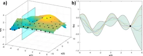
An illustration of a conditional simulation with two dimen-sional input space is presented in Fig. 1. Five possible condi-tional simulations of the 2D surface, considering the magnitude of deviation fixed at highlighted points, is shown superimposed in Fig. 1(a). Figure 1(b) shows the cross-section at the plane illustrated in Fig. 1(a).
The conditional simulation follows predetermined values at selected key points and the behaviour of the predicted surface between the key points is dependent on the parameters of the GRF whose optimised values are obtained for a given part as described in Section 2.1.2.
The uncertainty of the predicted deviation between key points is obtained as described in Section 2.2.3 and provides an envelope within which, statistically, all generated non-ideal part instances will lie with a given confidence. A 95% confi-dence interval on the mean value of generated deviations for the illustrated case is shown superimposed with the cross-sections in Fig. 1(b).
The variation of uncertainty in predicted deviations is physi-cally meaningful, as the shapes a part can take around the fixed key point is limited due to geometric covariance [27] and the possibilities increase as we move away from the key point. Ac-cordingly, the uncertainty of prediction is low near the key point and increases further away from it as shown in Fig. 1(b).
a) b)
Fig. 1: Conditional simulations (a) generated surfaces; (b) surface cross-sections at shown plane with 95% confidence interval on the mean of prediction
The proposed non-ideal part modelling methodology is schematically illustrated in Figs. 2 and 3, and has two main components: (1) Non-ideal part modelling, and (2) Non-ideal part generation.
2.1. Non-ideal part modelling
[image:2.595.307.558.539.637.2]func-CAD, GD&T
Non-ideal part representatives Data from
measurement or simulation
Discretised CAD (X) Find node deviation (Z) perpendicular to surface
Zf X
Model Zas a Gaussian random field, with Xas
input domain i.e.
Conditionally simulate non-ideal part instances
(Z|Z*,X) Select Key points
Cloud of Points (CoP) from measurement or
simulation
Set key points’ deviation (Z*)
Non-ideal part modelling (Section 2.1) Non-ideal part generation (Section 2.2)
[image:3.595.64.533.73.198.2]Section 2.1.1 Section 2.1.2 Section 2.2.1 Section 2.2.2
Fig. 2: Graphical illustration of methodology
Non-ideal partmodelling - Section 2.1
Non-ideal part generation-Section 2.2
Input pre-processing
CAD to Mesh representation
of part
Part measurement or Physical simulation
Obtain mesh nodes deviation information
Obtain optimum model parameters that characterize deviations..
Select Key Points
Estimate deviation of entire part
Required parts generated?
End Yes No
Set key point deviations
Fig. 3: Proposed non-ideal part modelling methodology
tion m(x) is defined asE[f(x)]. The covariance function be-tween two pointsxi,xj, on the surface of the part, represented
as,c(xi,xj) is defined asE[(f(xi)−m(xi))(f(xj)−m(xj))], where
Eis the expectation operator.
The mean function captures large scale trends in the devi-ation data and can be found by fitting regression models [28], or, by the maximisation of marginal likelihood as described in Section 2.1.2. In the study a zero mean function is utilised with-out affecting the analysis [25], as part variations are nominally
assumed to vary about zero mean.
The smoothness of generated deviations and the extent to which a given deviation propagates along a given direction (cor-relation length [25]), is characterised by the covariance function and its parameters. Covariance functions are classified as sta-tionary and non-stasta-tionary [22]. Areview on the types of co-variance functions with different characteristics can be found
in [25].
The choice of covariance function also affects the continuity
and differentiability of the generated non-ideal part
represen-tatives. While mean square continuity and differentiability of
the random field is easily expressed in terms of continuity of covariance function at the origin, that of generated non-ideal part instances is a complex function of covariance function as described in [24].
In the present study we choose the covariance function to characterise the GRF instead of the variogram traditionally used in geostatistics, due to the following advantages: (1) the ability to learn and model complex patterns in data with various com-binations of the covariance function [29], (2) the asymptotic properties of mean of covariance function parameters obtained in many settings through maximum likelihood estimation being equal to the true values of the parameters, and (3) the inability of the empirical semivariogram to distinguish the exact smooth-ness a differentiable process is [26].
For illustration purpose we choose the squared exponential covariance function represented by Eq. 1 where, for the three dimensional input case of non-ideal part modellingxis a 1×3 vector,σ2f is the signal variance or the scaling factor [25], and,
M is a 3×3 diagonal matrix with l−2, the inverse of square
of correlation lengths as diagonal. Representing byθthe set of all covariance function parameters{σ2f,l−2}. The aim of the
non-ideal part modelling phase is to find the optimumθthat fit the given part variation pattern, the optimised parameters are utilised during non-ideal part generation to emulate the part de-viation correlation.
c(xi,xj)=σ2fexp
−12(xi−xj)M(xi−xj)T
(1)
2.1.1. Input and pre-processing
Part variation data either in the form of physical simulation of manufacturing process (for instance from FEM analysis) or measurement of manufactured part, are utilised to obtain non-ideal part deviation from nominal. The CAD model of the part, for which non-ideal part is to be generated, is discretised to a mesh representation from which, utilising the part variation data, the deviation of each node from nominal is calculated util-ising routines in VRM software [30]. The nominal mesh node co-ordinates act as inputXto the model and surface normal de-viation of each node from the nominal, i.e. Z, is modelled as the function f(X) .
Statistical Modal Analysis (SMA) [17,18] utilises 3D-Discrete Cosine Transform (DCT) to decompose measurement data into linear combination of orthogonal modes. GMA has been ap-plied to optimise fixture design [19] and link manufacturing process parameters to part form variation [20].
[image:3.595.63.267.239.560.2]In addition to the inability of above mentioned deviation de-composition based methodologies to model local part deforma-tions, the modes used in the decomposition of deviation data, usually lie in a low dimensional space, which is not easily phys-ically interpretable. Additionally, the deviation decomposition methodologies require availability of measurement data, thus, cannot be used during early design phase. A summary of capa-bilities of all discussed non-ideal part form variation modelling methodologies is presented in Table 1.
Table 1: Capabilities of part form variation modelling methodologies
Methodologies Natural mode
decomposition [14]
Geometric Modal Analysis [15,16]
Skin Model Shapes [11][13]
Morphing mesh
[9]
Proposed approach
Par
t f
or
m
var
iat
ion
m
od
el
lin
g
ca
pa
bi
lit
ie
s
Represent global
deviation
Represent local
deviation
Ensure surface continuities at
edges
Probabilistic bounds on
deviation
As afore-discussed literature shows that the existing method-ologies individually lack the ability to: 1) model simultaneously both global and local deformation, (2) ensure surface continu-ities at edges, and (3) provide easy engineering interpretation of the model parameters, and thus, are not designer friendly. In the present paper, a conditional simulation based non-ideal part modelling and generation methodology is proposed. The methodology overcomes aforementioned drawbacks and in ad-dition introduces a novel probabilistic view on deviation mod-elling. The contributions of the study are: (1) the ability to generate both local and global part deformations, (2) a de-signer friendly/intuitive form variation generation methodology
with physically meaningful model parameters, and (3) provid-ing probabilistic bounds on generated part deviations.
The rest of the paper is organised as follows; Section 2 de-scribes the problem and the proposed methodology in detail. Section 3 provides details on the application of the proposed methodology on an automotive door component. Finally, Sec-tion 4 discusses conclusion and further research.
2. Problem formulation and methodology
This study proposes a non-ideal compliant sheet metal part shape error modelling and analysis methodology by condi-tional simulation of Gaussian Random Fields (GRF). Each non-ideal part instance is generated through conditional simulation, which is a spatially consistent Monte Carlo simulation with the goal of realistically mimicking spatial variation of the source deviations [21].
The deviation of the manufactured part from its nominal sur-face is modelled as a GRF, which is characterised by its mean
function and the covariance function. A detailed description of GRF can found in [22–26].
Representing the co-ordinates of nominal points on the sur-face of the part by a N×3 matrixX, and the surface normal deviation of the nominal points by aN×1 vectorZ. The devia-tionZ, is modelled as a GRFf(), withXas its input domain i.e.
Z = f(X), and non-ideal part instances are generated through
conditional simulation.
Conditional simulation is performed by fixing surface nor-mal deviations from nominal to predetermined values for prede-termined key points, and then predicting deviations of all other points for the rest of the part. Detailed explanation for selec-tion and setting of deviaselec-tions of key points is presented in Sec-tion 2.2.
An illustration of a conditional simulation with two dimen-sional input space is presented in Fig. 1. Five possible condi-tional simulations of the 2D surface, considering the magnitude of deviation fixed at highlighted points, is shown superimposed in Fig. 1(a). Figure 1(b) shows the cross-section at the plane illustrated in Fig. 1(a).
The conditional simulation follows predetermined values at selected key points and the behaviour of the predicted surface between the key points is dependent on the parameters of the GRF whose optimised values are obtained for a given part as described in Section 2.1.2.
The uncertainty of the predicted deviation between key points is obtained as described in Section 2.2.3 and provides an envelope within which, statistically, all generated non-ideal part instances will lie with a given confidence. A 95% confi-dence interval on the mean value of generated deviations for the illustrated case is shown superimposed with the cross-sections in Fig. 1(b).
The variation of uncertainty in predicted deviations is physi-cally meaningful, as the shapes a part can take around the fixed key point is limited due to geometric covariance [27] and the possibilities increase as we move away from the key point. Ac-cordingly, the uncertainty of prediction is low near the key point and increases further away from it as shown in Fig. 1(b).
a) b)
Fig. 1: Conditional simulations (a) generated surfaces; (b) surface cross-sections at shown plane with 95% confidence interval on the mean of prediction
The proposed non-ideal part modelling methodology is schematically illustrated in Figs. 2 and 3, and has two main components: (1) Non-ideal part modelling, and (2) Non-ideal part generation.
2.1. Non-ideal part modelling
func-a)
b)
mm
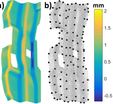
Fig. 4: a) Input pattern; b) Meshed part with key points
using the posterior covariance matrix (Eq. 4) to the mean values predicted (Eq. 3) utilising the conditional simulation methodol-ogy described in [21] which helps narrow the uncertainty by generating more probable non-ideal parts than the random vari-ations imparted by existing methodologies [10].
Non-ideal parts with a given probability of occurrence can be generated by addition of deviations (scaled according to the chosen probability using the variance of prediction) to mean surface. Such non-ideal parts when used in assembly enable probabilistic handling of variation propagation in manufactur-ing processes.
V(f(X)|X,X∗,Z∗) = C(X,X)−C(X,X∗) (C(X∗,X∗)+
σ2nI−1C(X∗,X) (4)
3. Case study
The proposed methodology is applied to automotive door hinge reinforcement. The part geometric deviation data is ob-tained from a single measurement of manufactured part and is illustrated in Fig. 4(a).
Firstly, the CAD model of the part for which non-ideal resentatives are to be generated is discretised to its mesh rep-resentation. The meshed representation of hinge reinforcement has approximately 12000 nodes as shown in Fig. 4(b). The de-viation at each node (Z∗) is found as described in Section 2.1.1.
The nominal position of all mesh node points in 3-dimensions forms the input X. In the case study a Matern covariance function with automatic relevance determination (ARD) [34] is used, and the optimum parametersθwere found by
maximis-ing the marginal likelihood (Eq. 2), through gradient descent utilising the routines provided in [35].
The generation of non-ideal parts as described in Section 2.2 is achieved through the manipulation of key points. The key points are selected to form a uniform grid structure covering the entire part, and are shown in Fig. 4b. The generated non-ideal part follows the key point, and the deviation between two key points mimics the original deviation pattern due the information carried by the covariance parametersθ.
The simulation of both local and global variations for the au-tomotive door hinge reinforcement with the moved key points
a)
b)
c)
mm
Fig. 5: a) Local defect at flanges; b) Local defect in the interior; c) Global defect - bending about illustrated axis
and corresponding non-ideal part generated is shown in Fig. 5. The key points inside the highlighted rectangles are given a de-viation of 2 mm in the surface normal direction for the simu-lation of local defects, where: Fig.5a illustrates defect affecting
the flanges, and Fig. 5(b) depicts a localised interior surface de-fect. Fig. 5(c) shows bending about an axis (a global defect), where all key points are imparted a deviation in the surface nor-mal direction to simulate a bending of 0.2 rad about the illus-trated axis.
The simulation of local defect is performed by moving only a few key points, in contrast for a global defect the deviation of all key points has to be specified depending on the type of defect to be simulated. Compound defects with both global and local deformations can be simultaneously simulated by su-perimposing the key point deviations corresponding to individ-ual defects. Similarly setting the key-point deviations to vary according to GD&T specifications enables simulation of non-ideal parts which conform to specific tolerance requirement.
It can be clearly seen from Fig. 5 that the longitudinal corre-lation patterns in the input pattern (Fig. 4a) is emulated by the generated deviations. This emulation of input correlation pat-terns enables the generated non-ideal part representatives to be realistic representations of manufactured part.
4. Conclusions
The non-ideal part modelling and generation methodology developed in this paper can model and generate most common part variations/defects that occur in sheet metals. The method-2.1.2. Model parameters optimisation
The covariance function parametersθ, as described in
Sec-tion 2.1, control smoothness and correlaSec-tion properties of the generated non-ideal part. The parameters are not as rigid as the coefficients in linear or non-linear regression models, in that a
given set of covariance function parameters can give rise to a large set of non-ideal parts.
The number of parameters (θ) depend on the type of co-variance function and on the number of coco-variance functions utilised to describe the random field. The optimum values of parametersθare found by maximising the likelihood given the part deviation data,L(θ|Z∗). The deviation data is obtained as
described in Section 2.1.1. An asterisk ∗ is used to represent
known node deviations, which during modelling stage is the set of all nodes. The method of obtaining the optimum covariance parameters by maximizing the marginal likelihood is robust and immune to over fitting [31]. In this study covariance function parameters are optimised from a single instance of non-ideal part data obtained as described in Section 3.
Finding the optimum parameters that characterise the given part variation enables accurate reproduction of source variation, as the behaviour of the generated non-ideal part between key points depends on the properties of the random field charac-terised by the parameters of the covariance function.
Traditionally, for mathematical ease of dealing with mul-tiplications of numbers of very small magnitudes, log likeli-hoods are used instead of likelilikeli-hoods, and since logarithm is a monotonically increasing function maximising log likelihood is also equivalent to maximising likelihood. For a GRF the log likelihood is given by Eq. 2 [26] where, C(θ) represents the N×Ndata covariance matrix which is obtained by applying the covariance function (for instance Eq.1) at all the mesh points of the nominal surface, |C(θ)|is the determinant of C(θ), and m(X∗) is the mean of the random field described in Section 2.1,
which is assumed to as zero in the study. ln(L(θ|Z∗)) = −N
2 ln(2π)−12ln(|C(θ)|)
−12(Z∗−m(X∗))TC(θ)−1(Z∗−m(X∗))
(2)
2.2. Non-ideal part generation
The optimum parameters of the covariance function char-acterising the variation of a given part, obtained as described in Section 2.1.2, are utilised to generate non-ideal part repre-sentatives using conditional simulation. Conditional simulation finds various possible instances of the variation for a given devi-ation setting of key points. The generated non-ideal part closely resembles the source variations from which the covariance pa-rameters were optimised, leading to realistic non-ideal part rep-resentatives. The main steps to generate non-ideal parts are: 1) key point selection, 2) key point deviation setting, and 3) devi-ation prediction of the entire part. These steps are explained in detail below.
2.2.1. Key point selection
Key points are the guiding points to generate different kinds
of variation, and are selected such that they uniformly cover the entire surface of the part. The key points also consist of the key characteristic points which are inspected during the assembly process. The non-ideal part generated by conditional simula-tion pass through the key point. Addisimula-tionally, selecting surface
edges as key points and setting their deviation values enable to overcome surface discontinuity issues, without any additional modelling efforts.
2.2.2. Key point deviation setting
Setting up the key points’ deviation is a critical step in the methodology enabling simulation of both global and local de-viations depending on the number of points manipulated. For instance, when a few points are moved as shown in Fig.5(a) and 5(b), local deformations can be simulated; and when all points are moved as shown in Fig.5(c), a global deformation can be simulated. Thus, the magnitude of deviation of the key points is dependent on design intent and the variation to be simulated. The process of setting deviations is intuitive for the designer as a given deviation at a point on the surface of the part can be obtained by moving the corresponding key point by the same magnitude. Various kinds of design intents, such as sensitivity of variation of a particular region of a part can be easily sim-ulated by manipulating the key points in corresponding region. The method also has the added advantage of eliminating guess-work around the degree and order of the regression, or requiring to limit to second order shapes.
2.2.3. Deviation prediction of the part
The non-ideal parts generated by conditional simulation take the deviation of key points as the fixed points through which the generated non-ideal part should pass through. The key point deviations set in Section 2.2.2, determine the type of variation i.e.global or local, to be simulated in non-ideal part instances. The mean deviation of the entire part after setting the key point deviations is generated through Gaussian Process Regres-sion (GPR) [25]. GPR is somewhat similar to the kriging ap-proach [32], which largely ignores probabilistic interpretation of the model and of the individual parameters of the covariance function [33].
The deviation of all mesh nodes of the part given a set of key point deviation is found using Eq. 3.Here:X∗, is theK×3
matrix of nominal key point co-ordinates where the deviation is set;X, is theN×3 matrix of nominal co-ordinates of all mesh points of the part where deviation is to be calculated;Z∗, is the
K×1 vector of key point deviations;I, is an identity matrix with size equal to the number of key points;C(X,X∗), is theN×K
covariance matrix with covariance function (Eq. 1) evaluated between each point inXandX∗;C(X∗,X∗), is theK×K
covari-ance matrix with covaricovari-ance function (Eq. 1) evaluated between each point inX∗;σ2
n, traditionally is the nugget effect [32] or
measurement error variance [25], which in the present non-ideal part modelling methodology is set to zero so that the generated non ideal part instances exactly pass through the key points. The optimum parameters of the covariance function character-ising the variation of a given part found in Section 2.1.2 are utilised to evaluate the covariance matrices in Eq. 3.
m(f(X)|X,X∗,Z∗)=C(X,X∗)C(X∗,X∗)+σ2
nI
−1
Z∗ (3)
a)
b)
mm
Fig. 4: a) Input pattern; b) Meshed part with key points
using the posterior covariance matrix (Eq. 4) to the mean values predicted (Eq. 3) utilising the conditional simulation methodol-ogy described in [21] which helps narrow the uncertainty by generating more probable non-ideal parts than the random vari-ations imparted by existing methodologies [10].
Non-ideal parts with a given probability of occurrence can be generated by addition of deviations (scaled according to the chosen probability using the variance of prediction) to mean surface. Such non-ideal parts when used in assembly enable probabilistic handling of variation propagation in manufactur-ing processes.
V(f(X)|X,X∗,Z∗) = C(X,X)−C(X,X∗) (C(X∗,X∗)+
σ2nI−1C(X∗,X) (4)
3. Case study
The proposed methodology is applied to automotive door hinge reinforcement. The part geometric deviation data is ob-tained from a single measurement of manufactured part and is illustrated in Fig. 4(a).
Firstly, the CAD model of the part for which non-ideal resentatives are to be generated is discretised to its mesh rep-resentation. The meshed representation of hinge reinforcement has approximately 12000 nodes as shown in Fig. 4(b). The de-viation at each node (Z∗) is found as described in Section 2.1.1.
The nominal position of all mesh node points in 3-dimensions forms the input X. In the case study a Matern covariance function with automatic relevance determination (ARD) [34] is used, and the optimum parametersθwere found by
maximis-ing the marginal likelihood (Eq. 2), through gradient descent utilising the routines provided in [35].
The generation of non-ideal parts as described in Section 2.2 is achieved through the manipulation of key points. The key points are selected to form a uniform grid structure covering the entire part, and are shown in Fig. 4b. The generated non-ideal part follows the key point, and the deviation between two key points mimics the original deviation pattern due the information carried by the covariance parametersθ.
The simulation of both local and global variations for the au-tomotive door hinge reinforcement with the moved key points
a)
b)
c)
mm
Fig. 5: a) Local defect at flanges; b) Local defect in the interior; c) Global defect - bending about illustrated axis
and corresponding non-ideal part generated is shown in Fig. 5. The key points inside the highlighted rectangles are given a de-viation of 2 mm in the surface normal direction for the simu-lation of local defects, where: Fig.5a illustrates defect affecting
the flanges, and Fig. 5(b) depicts a localised interior surface de-fect. Fig. 5(c) shows bending about an axis (a global defect), where all key points are imparted a deviation in the surface nor-mal direction to simulate a bending of 0.2 rad about the illus-trated axis.
The simulation of local defect is performed by moving only a few key points, in contrast for a global defect the deviation of all key points has to be specified depending on the type of defect to be simulated. Compound defects with both global and local deformations can be simultaneously simulated by su-perimposing the key point deviations corresponding to individ-ual defects. Similarly setting the key-point deviations to vary according to GD&T specifications enables simulation of non-ideal parts which conform to specific tolerance requirement.
It can be clearly seen from Fig. 5 that the longitudinal corre-lation patterns in the input pattern (Fig. 4a) is emulated by the generated deviations. This emulation of input correlation pat-terns enables the generated non-ideal part representatives to be realistic representations of manufactured part.
4. Conclusions
The non-ideal part modelling and generation methodology developed in this paper can model and generate most common part variations/defects that occur in sheet metals. The method-2.1.2. Model parameters optimisation
The covariance function parametersθ, as described in
Sec-tion 2.1, control smoothness and correlaSec-tion properties of the generated non-ideal part. The parameters are not as rigid as the coefficients in linear or non-linear regression models, in that a
given set of covariance function parameters can give rise to a large set of non-ideal parts.
The number of parameters (θ) depend on the type of co-variance function and on the number of coco-variance functions utilised to describe the random field. The optimum values of parametersθare found by maximising the likelihood given the part deviation data,L(θ|Z∗). The deviation data is obtained as
described in Section 2.1.1. An asterisk∗ is used to represent
known node deviations, which during modelling stage is the set of all nodes. The method of obtaining the optimum covariance parameters by maximizing the marginal likelihood is robust and immune to over fitting [31]. In this study covariance function parameters are optimised from a single instance of non-ideal part data obtained as described in Section 3.
Finding the optimum parameters that characterise the given part variation enables accurate reproduction of source variation, as the behaviour of the generated non-ideal part between key points depends on the properties of the random field charac-terised by the parameters of the covariance function.
Traditionally, for mathematical ease of dealing with mul-tiplications of numbers of very small magnitudes, log likeli-hoods are used instead of likelilikeli-hoods, and since logarithm is a monotonically increasing function maximising log likelihood is also equivalent to maximising likelihood. For a GRF the log likelihood is given by Eq. 2 [26] where, C(θ) represents the N×Ndata covariance matrix which is obtained by applying the covariance function (for instance Eq.1) at all the mesh points of the nominal surface,|C(θ)|is the determinant of C(θ), and m(X∗) is the mean of the random field described in Section 2.1,
which is assumed to as zero in the study. ln(L(θ|Z∗)) = −N
2 ln(2π)−12ln(|C(θ)|)
−12(Z∗−m(X∗))TC(θ)−1(Z∗−m(X∗))
(2)
2.2. Non-ideal part generation
The optimum parameters of the covariance function char-acterising the variation of a given part, obtained as described in Section 2.1.2, are utilised to generate non-ideal part repre-sentatives using conditional simulation. Conditional simulation finds various possible instances of the variation for a given devi-ation setting of key points. The generated non-ideal part closely resembles the source variations from which the covariance pa-rameters were optimised, leading to realistic non-ideal part rep-resentatives. The main steps to generate non-ideal parts are: 1) key point selection, 2) key point deviation setting, and 3) devi-ation prediction of the entire part. These steps are explained in detail below.
2.2.1. Key point selection
Key points are the guiding points to generate different kinds
of variation, and are selected such that they uniformly cover the entire surface of the part. The key points also consist of the key characteristic points which are inspected during the assembly process. The non-ideal part generated by conditional simula-tion pass through the key point. Addisimula-tionally, selecting surface
edges as key points and setting their deviation values enable to overcome surface discontinuity issues, without any additional modelling efforts.
2.2.2. Key point deviation setting
Setting up the key points’ deviation is a critical step in the methodology enabling simulation of both global and local de-viations depending on the number of points manipulated. For instance, when a few points are moved as shown in Fig.5(a) and 5(b), local deformations can be simulated; and when all points are moved as shown in Fig.5(c), a global deformation can be simulated. Thus, the magnitude of deviation of the key points is dependent on design intent and the variation to be simulated. The process of setting deviations is intuitive for the designer as a given deviation at a point on the surface of the part can be obtained by moving the corresponding key point by the same magnitude. Various kinds of design intents, such as sensitivity of variation of a particular region of a part can be easily sim-ulated by manipulating the key points in corresponding region. The method also has the added advantage of eliminating guess-work around the degree and order of the regression, or requiring to limit to second order shapes.
2.2.3. Deviation prediction of the part
The non-ideal parts generated by conditional simulation take the deviation of key points as the fixed points through which the generated non-ideal part should pass through. The key point deviations set in Section 2.2.2, determine the type of variation i.e.global or local, to be simulated in non-ideal part instances. The mean deviation of the entire part after setting the key point deviations is generated through Gaussian Process Regres-sion (GPR) [25]. GPR is somewhat similar to the kriging ap-proach [32], which largely ignores probabilistic interpretation of the model and of the individual parameters of the covariance function [33].
The deviation of all mesh nodes of the part given a set of key point deviation is found using Eq. 3.Here:X∗, is theK×3
matrix of nominal key point co-ordinates where the deviation is set;X, is theN×3 matrix of nominal co-ordinates of all mesh points of the part where deviation is to be calculated;Z∗, is the
K×1 vector of key point deviations;I, is an identity matrix with size equal to the number of key points;C(X,X∗), is theN×K
covariance matrix with covariance function (Eq. 1) evaluated between each point inXandX∗;C(X∗,X∗), is theK×K
covari-ance matrix with covaricovari-ance function (Eq. 1) evaluated between each point inX∗;σ2
n, traditionally is the nugget effect [32] or
measurement error variance [25], which in the present non-ideal part modelling methodology is set to zero so that the generated non ideal part instances exactly pass through the key points. The optimum parameters of the covariance function character-ising the variation of a given part found in Section 2.1.2 are utilised to evaluate the covariance matrices in Eq. 3.
m(f(X)|X,X∗,Z∗)=C(X,X∗)C(X∗,X∗)+σ2
nI
−1
Z∗ (3)
[image:5.595.312.555.73.390.2] [image:5.595.70.265.75.254.2]ology requires very few parameters to be determined by hand and the generated part form variations are similar to the source variation in terms of covariance of generated deviations, un-like random variations which existing methodologies generate. The characterisation of deviation is automatically performed by maximising the marginal likelihood, without requiring the tun-ing of many parameters or manual parameter guesstun-ing. The methodology is also able to model and generate non-ideal parts from a single non-ideal part data instance.
Additionally, the methodology provides: (1) probabilistic bounds on generated variation enabling us to deal with varia-tion propagavaria-tion in a probabilistic way, and (2) characterisa-tion of covariance parameters enables generalizing the variacharacterisa-tion across different parts manufactured from a given process.
How-ever, a known issue with GPR is the increase in computational cost involved with invertingN×Nmatrix, where N represents the number of known data points. As future work we aim to: (1) develop a mapping from covariance function parameters to the manufacturing process parameters enabling the simulation of non-ideal part truly independent of data, either measurement or simulation; and (2) extend the methodology to characterise the non-ideal part variation in a batch of parts.
Acknowledgements
This study has been supported by the UK EPSRC project EP/K019368/1: “ Self-Resilient Reconfigurable Assembly
Sys-tems with In-process Quality Improvement.”
References
[1] U. Roy, C. Liu, T. Woo, Review of dimensioning and tolerancing: repre-sentation and processing, Computer-Aided Design (1991) 466–483. [2] W. Polini, Taxonomy of models for tolerance analysis in assembling,
International Journal of Production Research 50 (7) (2012) 2014–2029. doi:10.1080/00207543.2011.576275.
[3] H. Chen, S. Jin, Z. Li, X. Lai, A comprehensive study of three dimen-sional tolerance analysis methods, Computer-Aided Design 53 (2014) 1– 13. doi:10.1016/j.cad.2014.02.014.
[4] R. S. Pierce, D. Rosen, A Method for integrating form errors into geometric tolerance analysis, Journal of Mechanical Design 130 (1) (2007) 11002. doi:10.1115/1.2803252.
[5] J. Grandjean, Y. Ledoux, S. Samper, H. Favreli`ere, Form errors impact in a rotating plane surface assembly, Procedia CIRP 10 (2013) 178–185. doi:10.1016/j.procir.2013.08.029.
[6] J. Grandjean, Y. Ledoux, S. Samper, On the role of form defects in as-semblies subject to local deformations and mechanical loads, International Journal of Advanced Manufacturing Technology 65. doi:10.1007/ s00170-012-4298-6.
[7] S. L. Semiatin, E. MArquard, H. Lampman, ASM Handbook: Metalwork-ing - sheet formMetalwork-ing, Vol. 14, ASM international, 2006.
[8] P. Borrel, A. Rappoport, Simple constrained deformations for geometric modeling and interactive design, ACM Transactions on Graphics 13 (2) (1994) 137–155. doi:10.1145/176579.176581.
[9] P. Franciosa, S. Gerbino, S. Patalano, Simulation of variational compliant assemblies with shape errors based on morphing mesh approach, The Inter-national Journal of Advanced Manufacturing Technology 53 (1-4) (2010) 47–61. doi:10.1007/s00170-010-2839-4.
[10] B. Schleich, N. Anwer, L. Mathieu, S. Wartzack, Skin Model Shapes: A new paradigm shift for geometric variations modelling in mechanical engineering, Computer-Aided Design 50 (2014) 1–15. doi:10.1016/j.cad.2014.01.001.
[11] ISO-17450, ISO 17450-1:2011, Geometrical product specifications (GPS) General concepts Part 1 : Model for geometrical specification (2011). [12] M. Zhang, N. Anwer, A. Stockinger, L. Mathieu, S. Wartzack, Discrete
shape modeling for skin model representation, Proceedings of the
Institu-tion of Mechanical Engineers, Part B: Journal of Engineering Manufacture 227 (5) (2013) 672–680. doi:10.1177/0954405412466987.
[13] X. Yan, A. Ballu, Toward an automatic generation of part models with form error, Procedia CIRP 43 (2016) 23–28. doi:10.1016/j.procir.2016.02.109.
[14] S. Samper, F. Formosa, Form defects tolerancing by natural modes anal-ysis, Journal of Computing and Information Science in Engineering 7 (1) (2007) 44. doi:10.1115/1.2424247.
[15] A. Das, P. Franciosa, P. Prakash, D. Ceglarek, Transfer function of as-sembly process with compliant non-ideal parts, Procedia CIRP 21 (2014) 177–182. doi:10.1016/j.procir.2014.03.195.
[16] A. Das, Shape variation modelling, analysis and statistical control for as-sembly system with compliant parts, Ph.D. thesis, University of Warwick (2016).
[17] W. Huang, Methodologies for modelling and analysis of stream of variation in compliant and rigid assemblies, Ph.D. thesis, University of Wisconsin-Madison (2004).
[18] W. Huang, J. Liu, V. Chalivendra, D. Ceglarek, Z. Kong, Y. Zhou, Sta-tistical modal analysis for variation characterization and application in manufacturing quality control, IIE Transactions 46 (5) (2014) 497–511. doi:10.1080/0740817X.2013.814928.
[19] A. Das, P. Franciosa, D. Ceglarek, Fixture design optimisation considering production batch of compliant non-ideal sheet metal parts, Procedia Man-ufacturing 1 (MAY) (2015) 157–168. doi:10.1016/j.promfg.2015.09.079.
[20] A. Das, P. Franciosa, A. Pesce, S. Gerbino, Parametric effect analysis of
free-form shape error during sheet metal forming parametric effect analysis
of free-form shape error during sheet metal forming, International Journal of Engineering Science and Technology (IJEST) 9 (September). [21] J.-P. Chiles, P. Delfiner, Geostatistics: modeling spatial uncertainty, Vol.
497, John Wiley & Sons, 2009.
[22] E. Vanmarcke, Random fields: Analysis and synthesis, MIT Press Cam-bridge, MA., 1983.
[23] R. J. Adler, The geometry of random fields, Society for Industrial and Ap-plied Mathematics, 2010. doi:10.1137/1.9780898718980.
[24] R. J. Adler, R. J. Adler, J. E. Taylor, K. J. Worsley, Applications of random fields and geometry: foundations and case studies, 2010.
[25] C. E. Rasmussen, C. K. Williams, Gaussian processes for machine learn-ing, Vol. 1, MIT press Cambridge, 2006.
[26] M. L. Stein, Interpolation of spatial data: some theory for kriging, Springer Science & Business Media, 2012.
[27] K. G. Merkley, Tolerance analysis of compliant assemblies, Ph.D. thesis, Brigham Young University (1998).
[28] N. Cressie, C. K. Wikle, Statistics for spatio-temporal data, Wiley, 2011. [29] D. Duvenaud, J. R. Lloyd, R. Grosse, J. B. Tenenbaum, Z. Ghahramani,
Structure discovery in nonparametric regression through compositional kernel search, Proceedings of the 30th International Conference on Ma-chine Learning 30 (2013) 1166–1174. arXiv:arXiv:1302.4922v4. [30] P. Franciosa, D. Ceglarek, Fixture analyser & optimiser (2017).
URL http://www2.warwick.ac.uk/fac/sci/wmg/research/ manufacturing/downloads/
[31] D. J. C. MacKay, Bayesian interpolation, Neural Computation 4 (3) (1992) 415–447. doi:10.1162/neco.1992.4.3.415.
[32] J.-P. Chiles, P. Delfiner, Geostatistics: modeling spatial uncertainty, 2nd Edition, Wiley-Blackwell, 2011.
[33] D. J. MacKay, Introduction to gaussian processes, NATO ASI Series F Computer and Systems Sciences 168 (1998) 133–166.
[34] R. M. Neal, Bayesian learning for neural networks, Springer New York, 1996.
[35] C. E. Rasmussen, H. Nickisch, The GPML Toolbox version 3 . 2, Toolbox (2013) 1–32.