Nonnegative Matrix Factorization Requires Irrationality∗
Dmitry Chistikov†, Stefan Kiefer‡, Ines Maruˇsi´c‡, Mahsa Shirmohammadi‡, and James Worrell‡
Abstract. Nonnegative matrix factorization (NMF) is the problem of decomposing a given nonnegativen×m
matrix M into a product of a nonnegativen×dmatrixW and a nonnegatived×mmatrix H. A longstanding open question, posed by Cohen and Rothblum in 1993, is whether a rational matrix
M always has an NMF of minimal inner dimensiondwhose factorsW andH are also rational. We answer this question negatively, by exhibiting a matrix for whichWandHrequire irrational entries.
Key words. nonnegative matrix factorization, nonnegative rank
AMS subject classifications. 15B48, 15A23, 52B05, 68T30, 68Q99
DOI. 10.1137/16M1078835
1. Introduction. Nonnegative matrix factorization (NMF) is the task of factoring a ma-trix of nonnegative real numbersM(henceforth anonnegative matrix) as a productM =W·H
such that the matrices W and H are also nonnegative. As well as being a natural problem in its own right (see Thomas [26] and Cohen and Rothblum [9]), NMF has found many ap-plications in various domains, including machine learning, combinatorics, and communication complexity; see, e.g., [3,13,18,19,28,29] and the references therein.
For an NMFM =W·H, the number of columns inW is called theinner dimension. The smallest inner dimension of any NMF ofMis called thenonnegative rank (over the reals)ofM; an early reference is the paper by Gregory and Pullman [15]. Similarly, thenonnegative rank ofM over the rationals is defined as the smallest inner dimension of an NMFM =W·Hwith matrices W, H that have only rational entries. Cohen and Rothblum [9] posed the following problem in 1993:
“Problem. Show that the nonnegative ranks of a rational matrix over the reals and over the rationals coincide, or provide an example where the two ranks are different.”
In this paper, we solve the above problem by providing an example of a rational matrix M
that has different nonnegative ranks overR and over Q.
∗
Received by the editors June 7, 2016; accepted for publication (in revised form) March 10, 2017; published electronically June 29, 2017. The initial version of this paper appeared online as a technical report on arXiv [6]. Extended abstracts of parts of the paper previously appeared in conference proceedings as [7] and [8].
http://www.siam.org/journals/siaga/1/M107883.html
Funding: The first author’s work was sponsored in part by the ERC Synergy award ImPACT and was supported by ERC grant AVS-ISS (648701). The second author’s work was supported by a University Research Fellowship of the Royal Society and by the EPSRC. The work of the third, fourth, and fifth authors was supported by the EPSRC.
†
Max Planck Institute for Software Systems (MPI-SWS), Kaiserslautern 67663 and Saarbr¨ucken 66123, Germany. Current address: University of Warwick, Coventry CV4 7AL, UK ([email protected]).
‡
University of Oxford, Oxford OX1 3QD, UK ([email protected], [email protected], mahsa. [email protected],[email protected]).
285
Discussion. In the last few years, there has been progress towards resolving the Cohen– Rothblum problem. It was already known to Cohen and Rothblum [9] that the nonnegative ranks over R and Q coincide for matrices of rank at most 2. (Note that the usual ranks
overRand Qcoincide for all rational matrices.) In 2015, Kubjas, Robeva, and Sturmfels [16,
Corollary 4.6] extended this result to matrices of nonnegative rank (overR) at most 3. On the
other hand, Shitov [22] proved that the nonnegative rank of a matrix can indeed depend on the underlying field: he exhibited a nonnegative matrix with irrational entries whose nonnegative rank over a subfield of R is different from its nonnegative rank over R. Independently and
concurrently with our work [6], Shitov [23] also proposes a rational matrix whose nonnegative ranks overR andQ are different.
In the present paper, in order to find a rational matrix that has different nonnegative ranks overRandQ, we proceed in two steps. In the first step, we studyrestricted NMFs [14],
that is, those factorizationsM0 =W·H0 of a given matrixM0 in which the columns ofW span the same vector space as the columns ofM0. We find irrationality in this setting, constructing a rational matrix M0 that has a unique (and irrational) restricted NMFM0=W·H0 of inner dimension 5; uniqueness here is understood up to permutation and rescaling of columns ofW. In the second step, we transfer this irrationality to our main setting: we construct, based on the matrix M0, another matrix M that has a unique (and irrational) NMF M = W ·H of inner dimension 5.
For the first step, it has long been known [9] that NMF can be interpreted geometrically as finding a set of vectors (columns of W) inside a unit simplex whose convex hull contains a given set of points (columns of M). It has recently been shown by Gillis and Glineur [14] (see also [7]) that restricted NMFs are in one-to-one correspondence withnested polytopes: a matrixM0 corresponds to a pair of full-dimensional polytopesR ⊆ P, and a restricted NMF of M0 corresponds to a polytope Q nested in between: R ⊆ Q ⊆ P. In this paper we find a pair of 3-dimensional polytopes R ⊆ P with rational vertices such that there is only one 5-vertex polytope Q with R ⊆ Q ⊆ P, and the vertices of this polytope Q have irrational coordinates: R and P are chosen so as to impose quadratic constraints on the coordinates of the vertices of Q. This gives us a rational matrix M0 that has a unique (and irrational) restricted NMFM0 =W ·H0 of inner dimension 5.
For the second step, if we knew that the factorization M0 =W ·H0 were unique among all NMFs of the same inner dimension, we would be done. This, however, requires ruling out several classes of other hypothetical (nonrestricted) factorizations of the matrix.
Towards this goal, one might want to take advantage of the work on uniqueness properties of NMF, studied, for instance, by Thomas [26], Laurberg et al. [17], and Gillis [12], or on the topology of the set of all NMFs (see Mond, Smith, and van Straten [20]). Here we pursue a different strategy. We show that for a larger matrix M = M0 Wε
, where Wε
is a nonnegative rational matrix which is entrywise close to W, the only NMF (restricted or otherwise) of the same inner dimension has the same left factor W—thus extending the uniqueness property to the nonrestricted setting.
The guiding idea behind our extending M0 to M is that by including all columns of W
in the set of columns of M, we can exclude certain “undesirable” factorizations, thereby ensuring thatM has no rational NMF. We show this by a constraint propagation argument. Unfortunately for this construction, the matrix W itself has irrational entries. However, we
show that we can instead take any nonnegativerational matrixWε within a sufficiently small
neighborhood of W, and the undesirable factorizations will still be excluded. In the text we describe such a neighborhood explicitly and pick a specific rational matrix Wε from it, thus
obtaining the matrixM of the above form and proving the main result of the paper.
Conceptually, the existence of a suitable matrixWε can be understood in terms ofupper
semicontinuity of the nonnegative rank overR, proved by Bocci, Carlini, and Rapallo [4]. By
this property, if a matrix M has nonnegative rank r over R, then all nonnegative matrices
in a sufficiently small neighborhood of M have nonnegative rank r or greater (over R). In
the same manner, our proof extends the nonexistence of undesirable factorizations from the matrixW toWε.
From the computational perspective, nonnegative rank (over R as well as over Q) is a
nontrivial quantity to compute. The usual rank of a matrix M is greater than or equal tor
if and only if M has an r×r submatrix of rank r. The same property does not hold for nonnegative rank. This follows from a construction by Moitra [19] of a family of matrices, indexed by r, n∈N, respectively having size 3rn×3rnand nonnegative rank at least 4r, but
no (n−1)×3rnsubmatrix of nonnegative rank greater than 3r. A strengthening of this result can be found in Eggermont, Horobet, and Kubjas [11]; this paper, in fact, studies the set of matrices of nonnegative rank at most 3 and looks into the properties of the boundary of this set.
Deciding whether a given matrix has nonnegative rank at most r is a computationally hard problem, known to be NP-hard due to a result by Vavasis [27]. The problem is easily seen to be reducible to the decision problem for the existential theory of real closed fields and therefore belongs toPSPACE(see, e.g., [5]). Beyond this generic upper bound, the problem has been attacked from many different angles. Here we highlight the results of Arora et al. [2], who identified several variants of the problem that are efficiently solvable, and Moitra [19], who found semialgebraic descriptions of the sets of matrices of nonnegative rank at mostr in which the number of variables is O(r2). However, it remains an open question [27] whether or not the set{(M, r) : the nonnegative rank of M is ≤r}belongs toNP; our solution to the Cohen–Rothblum problem does not exclude either possibility (even though it does rule out a hypothetical “simple” argument for membership inNP, wherein a certificate is an NMF with rational entries of small bit size).
2. Preliminaries. For any ordered fieldF, we denote by F+ the set of all its nonnegative
elements. For any vectorv, we writevi for its ith entry. A vector of real numbers v is called
pseudostochastic if its entries sum up to one. A pseudostochastic vectorv is called stochastic if its entries are nonnegative.
For any matrix M, we writeMi,: for itsith row,M:,j for itsjth column, and Mi,j for its
(i, j)th entry. A matrix is callednonnegative if all its entries are nonnegative, it is called ratio-nal if all its entries are rational, and it is calledzero if all its entries are zero. A nonnegative matrix is stochastic if its columns are stochastic.
2.1. Nonnegative rank. LetFbe an ordered field, such as the realsRor the rationalsQ.
Given a nonnegative matrix M ∈ Fn+×m, a nonnegative matrix factorization (NMF) over F
of M is any representation of the form M = W ·H, where W ∈ Fn+×d and H ∈ Fd ×m
+ are
nonnegative matrices. We refer to das the inner dimension of the NMF, and hence refer to
NMFM =W ·H as beingd-dimensional. Thenonnegative rank over F ofM is the smallest
nonnegative integer d such that there exists a d-dimensional NMF over F of M. We may
equivalently characterize [9] the nonnegative rank over F of M as the smallest number of
rank-1 matrices inFn+×m such thatM is equal to their sum. The nonnegative rank overRwill
henceforth simply be called nonnegative rank. For any nonnegative matrix M ∈Rn+×m, it is
easy to see that rank(M) ≤rank+(M) ≤min{n, m}, where rank(M) and rank+(M) denote
the rank and the nonnegative rank, respectively. Given a nonzero matrix M ∈ Fn×m
+ , by removing the zero columns of M and dividing
each remaining column by the sum of its elements, we obtain a stochastic matrix with equal nonnegative rank. Similarly, if M =W ·H, then after removing the zero columns inW and multiplying with a suitable diagonal matrixD, we getM =W·H=W D·D−1H,whereW D
is stochastic. If M is stochastic, then (writing 1for a row vector of ones) we have
1=1M =1W D·D−1H =1D−1H,
and henceD−1His stochastic as well. Thus, without loss of generality one can consider NMFs
M = W ·H in which M, W, and H are all stochastic matrices [9, Theorem 3.2]. In such a case, we will call the factorizationM =W ·H stochastic.
2.2. Nested polygons in the plane. In this paper all polygons are assumed to be convex. Given two polygons in the plane, R ⊆ P ⊆R2, a polygon Q is said to be nested between R
and P if R ⊆ Q ⊆ P. Such a polygon is said to be minimal if it has the minimum number of vertices among all polygons nested between R and P. In this section we recall from [1] a standardized form for minimal nested polygons, which will play an important role in the subsequent development.
Fix two polygons R and P, with R ⊆ P. A supporting line segment is a directed line segmentuvsuch that, first, the endpointsu andvlie on the boundary of the outer polygonP
and, second, the inner polygonRtouchesuvand lies to the left ofuv. A nested polygon with vertices v1, . . . , vk, listed in counterclockwise order, is said to be supporting if the directed
line segments v1v2, v2v3, . . . , vk−1vk are all supporting. (Note that the directed line segment
vkv1need not be supporting.) Such a polygon is uniquely determined by the vertexv1 (see [1,
section 2]) and is henceforth denoted bySv1. It is shown in [1] that some supporting polygon
is also minimal. More specifically, from [1, Lemma 4] we have the following lemma.
Lemma 2.1. Consider a minimal nested polygon with vertices v1, . . . , vk, listed in
counterclockwise order, where v1 lies on the boundary of P. The supporting polygon Sv1
is also minimal.
We will need the following elementary fact of linear algebra in connection with subsequent applications of Lemma2.1. Letv1 = (x1, y1),v2 = (x2, y2), andv3 = (x3, y3) be three distinct points in the plane, and consider the determinant
∆ =
x1 y1 1
x2 y2 1
x3 y3 1
.
Then ∆ = 0 if and only if v1,v2, andv3 belong to some common line, and ∆>0 if and only if the list of verticesv1, v2, v3 describes a triangle with counterclockwise orientation.
3. Main result. We show that the nonnegative ranks over R and Q are, in general,
dif-ferent.
Theorem 3.1. Let M = M0 Wε
∈Q6×11+ , where
M0 = 5 44 5 11 85
121 0 0 0
0 0 0 112 113 337
1 11 1 44 2 121 1 44 15 88 17 88 1 44 1 44 8 121 1 44 19 88 5 24 3 11 3 11 12 121 8 11 2 11 2 33 1 2 5 22 14 121 1 22 7 44 43 132
∈Q6×6+ ,
Wε=
0 133165 2233640 0 0
1
111540 0 0
17209 58047 997 5082 114721 892320 1 146850 17 506 385 1759 2921 203280 47 1248 413 5874 1 102718 2915 10554 4381 203280 36 169 22 267 18674 51359 1 116094 3252 4235 276953 446160 1009 24475 16239 51359 1100 5277 1 101640
∈Q6×5+ .
The nonnegative rank of M over R is 5. The nonnegative rank of M over Qis 6.
The rest of this paper is devoted to the proof of Theorem3.1.
The matrix M is stochastic. The matrix M0 has a stochastic 5-dimensional NMF
M0=W ·H0 withW,H0 as follows:
W =
0 57 +5
√ 2 77
15+5√2
77 0 0
0 0 0 20+2
√ 2 77
48−8√2 187 √
2
11 0
4−√2 77 3 14+ √ 2 308
14−8√2 187 −1+√2
11
4+√2
77 0
39 154+
5√2 308
21−12√2 187 8−4√2
11
12−4√2 77
4
11 0
104+28√2 187 4+2√2
11
6−2√2 77
30−4√2 77 3 11− √ 2 22 0 , (1)
H0 =
1+√2
4 0 √ 2 11 1 4 − √ 2 8 0 1 6+ √ 2 12
0 12 − √
2 8 1−
√ 2
11 0 0 0
3−√2 4
1 2 +
√ 2
8 0 0 0 0
0 0 0 0 2134+7
√ 2 68 5 6− √ 2 12
0 0 0 34 +
√ 2 8
13 34−
7√2 68 0 .
The matrix Wε has a stochastic 5-dimensional NMF Wε =W ·Hε withHε as follows:
30419 40560+
28679√2 162240
−2728 46725 +
5791√2 140175
2741 98049−
642√2 32683
−689 10554+
15595√2 337728
389 1848 −
5501√2 36960
0 163318140175 −7277 √
2 62300
5958 32683−
50543√2
392196 0 0
0 −213720025 + 6047
√ 2 80100
11062 14007+
8321√2
56028 0 0
7443 8840 −
51313√2
86190 0 0
148897 179418 +
172627√2 1435344
−1741 26180 +
1847√2 39270 −408157
689520 +
1154473√2
2758080 0 0
7039 29903−
318541√2 1913792
134461 157080+
1163√2 11424
.
Hence, the matrix M has a stochastic 5-dimensional NMF as follows:
(2) M =W · H0 Hε
.
We refer the reader to [30] for a Maple worksheet with calculations of the paper.
Remark 3.2. The columns of M and W span the same vector space. It follows that the restricted nonnegative ranks ofM overRandQare 5 and 6, respectively. In fact, the authors
of this paper previously exhibited a rational nonnegative matrix whose restricted nonnegative ranks overR andQ differ [7].
We fix the matricesM, M0, Wε, W, H0, Hε for the remainder of the paper.
3.1. Types of factorizations. LetM =L·R be a stochastic NMF of inner dimension at most 5. (As argued in section2.1, without loss of generality we may consider only stochastic NMFs of M.) Let us introduce the following notation:
• kis the number of columns in L whose first and second coordinates are 0,
• k1 is the number of columns inLwhose first coordinate is strictly positive and second
coordinate is 0, and
• k2 is the number of columns inLwhose second coordinate is strictly positive and first coordinate is 0.
Clearly, the factorizationM =L·Rcorresponds to representing each column ofM as a convex combination of the columns ofL, with the coefficients of the convex combination specified by the entries ofR. AsLhas at most five columns,
(3) k+k1+k2 ≤5.
Since the columns M:,1, M:,2, M:,3 are linearly independent, the matrix L has at least three
columns whose second coordinate is 0. Likewise, since the columnsM:,4, M:,5, M:,6 are linearly
independent,L has at least three columns whose first coordinate is 0. That is,
(4) k+k1≥3 and k+k2 ≥3.
Together with (3), this implies that 2k≥6−k1−k2 ≥1 +k, and therefore k≥1.
The columns M:,1, M:,2, M:,3 have first coordinate strictly positive and second
coordi-nate 0, while the columns M:,4, M:,5, M:,6 have second coordinate strictly positive and first
coordinate 0. Therefore, in order for these columns to be covered by columns of L, we need to have
(5) k1≥1 and k2 ≥1.
0 + + 0 0
0 0 0 + + · · · · · · · · · · · · · · · · · · · ·
type 1
0 0 + · ·
0 0 0 + + · · · · · · · · · · · · · · · · · · · ·
type 2
0 0 0 + +
0 0 + · · · · · · · · · · · · · · · · · · · · · ·
type 3
+ 0 0 0 0
0 + 0 0 0 · · · · · · · · · · · · · · · · · · · ·
[image:7.612.76.514.88.195.2] type 4
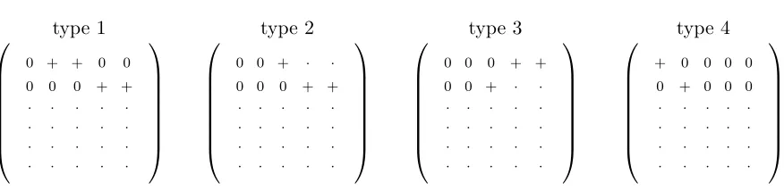
Figure 1. In any5-dimensional NMFM=L·R, the matrixLmatches one of the four patterns above, up to a permutation of its columns. Here+denotes any strictly positive number.
Together with (3), this implies thatk≤5−k1−k2≤3. We conclude thatk∈ {1,2,3}. More precisely, it is now a consequence of inequalities (3), (4), and (5) that the NMF M = L·R
has (at least) one of the following fourtypes: 1. k= 1,k1= 2, k2 = 2;
2. k= 2,k1= 1, k2 ∈ {0,1,2};
3. k= 2,k2= 1, k1 ∈ {0,1,2};
4. k= 3,k1= 1, k2 = 1.
These four types are illustrated in Figure1 for NMFs of inner dimension 5. In section4 we prove the following proposition.
Proposition 3.3. Let M be the matrix from Theorem3.1 and W the matrix from (1). 1. If M =L·R is a type-1 NMF, thenW:,1 is a column ofL, and thusL is not rational.
2. The matrix M has no type-2 NMF. 3. The matrix M has no type-3 NMF. 4. The matrix M has no type-4 NMF.
Using this proposition, we can prove Theorem 3.1.
Proof of Theorem 3.1. Due to the NMF ofMstated in (2), the nonnegative rank ofM is at most 5. If there existed an at most 4-dimensional NMF ofM,then, ask+k1+k2≤4, it would have to have type 2 or 3, but those types are excluded by items 2 and 3 of Proposition 3.3. Hence the nonnegative rank ofM overR equals 5.
Since M =I·M (whereI denotes the 6×6 identity matrix), the nonnegative rank of M
over Q is at most 6. By Proposition 3.3 there is no 5-dimensional NMF M =L·R with L
rational. Hence, the nonnegative rank ofM overQequals 6.
4. Proof of Proposition 3.3. It remains to prove Proposition 3.3. To rule out type-4 NMFs, we use constraint propagation in order to prove that the inequalities required for type-4 NMFs are contradictory; see section4.5. To rule out rational NMFs of types 1, 2, and 3, we employ geometric arguments concerning nested polygons in the plane (see sections 4.2–4.4). These arguments rely on a geometric interpretation of the specific NMF M =W · H0 Hε
given by (2). More precisely, we define a polytopeP ⊆R3, shown in Figure2, such that each
of the columns ofM and W can be associated with a point in P. The points associated with the columns of M lie in the convex hull of those associated with the columns ofW (cf. [14]).
4.1. Geometry behind the proof of Proposition3.3. To set up this geometric connection, observe that the matrixM is stochastic and has rank 4, and hence the columns ofM affinely span a 3-dimensional affine subspaceV ⊆R6. All vectors in V are pseudostochastic. The set
of stochastic vectors in V (equivalently, the nonnegative vectors in V) form a 3-dimensional polytope, say P0 ⊆ V. Clearly we haveM:,i∈ P0 for eachi∈ {1, . . . ,11}.
Parameterization. We will now fix a particular parameterization ofV andP0; that is, we define an injective affine function f :R3 →R6 and a polytopeP ⊆R3 such that f(R3) = V
and f(P) =P0. Letf :
R3 →R6 be the function with f(x) =Cx+dfor each x∈R3, where
C= 1 11 ·
0 10 0 0 0 4
−1 −2 1/2
−1 0 5/2 4 0 0
−2 −8 −7
∈Q6×3 and d= 1
11 · 0 0 2 1 0 8
∈Q6×1.
Note that the map f is injective. Defining
r1 =
3/4 1/8 0
, r2=
3/4 1/2 0
, r3 =
3/11 17/22
0
, r4 =
2 0 1/2
, r5 =
1/2
0 3/4
, r6=
1/6
0 7/12
,
we have f(ri) =M:0,i for each i∈ {1,2, . . . ,6}, and defining
q1ε= 99 169 0 1 40560 , q
ε 2= 121 534 133 150 0 , q
ε 3 = 9337 9338 64 203 0 , q
ε 4 = 1 42216 0 17209 21108 , q
ε 5 = 813 385 0 997 1848 ,
we have f(qiε) = (Wε):,i for each i ∈ {1,2, . . . ,5}. Thus, all columns of M lie in the image
of f. It follows that f(R3) =V.
Let P be the 3-dimensional polytope defined by {x∈R3 |f(x)≥0}. Then f(P) = P0.
Furthermore, ri ∈ P, as f(ri) = M:0,i∈ P0 for all i∈ {1,2, . . . ,6}. Likewise we have qiε ∈ P,
asf(qε
i) = (Wε):,i∈ P0 for all i∈ {1,2, . . . ,5}.
Figure 2 visualizes P, which has 6 faces corresponding to the inequalities of the system
Cx+d≥0. In more detail, P is the intersection of the following half-spaces: y ≥0 (blue),
z ≥ 0 (brown), −12x−y+ 14z+ 1 ≥ 0 (green), −x+ 52z + 1 ≥ 0 (yellow), x ≥ 0 (pink),
−14x−y−78z+ 1 ≥0 (transparent front). The figure also shows the position of the points
r1, . . . , r6 (black dots).1
In fact, the columns of W are also inP0 ⊆ V. Indeed, defining
q∗1 =
2−√2 0 0
, q
∗ 2 =
3−√2 7 11+√2
14
0
, q
∗ 3 = 1
3+√2 14
0
, q
∗ 4 = 0 0
10+√2 14
, q
∗ 5 =
26+7√2 17
0
12−2√2 17
,
1
In [7] the authors of the current paper used the same polytopeP and the same points r1, . . . , r6 (see
Figure2) to prove a related result about therestricted nonnegative rank.
x y
z
x y
[image:9.612.134.453.89.219.2]z
Figure 2. The two images show orthogonal projections of the3-dimensional polytope P. The black dots indicate 6 interior points: 3 points (r1, r2, r3) on the brown xy-face, and 3 points (r4, r5, r6) on the blue xz-face. (The images form a stereo pair intended for “parallel-eye” watching: to see the polytope in3D, look at the left and right projections with your left and right eyes, respectively, at the same time, as described, e.g., in[25].)
we havef(q∗i) =W:,i ∈ P0, and henceq∗i ∈ P for eachi∈ {1,2, . . . ,5}. That is, in our NMF
M = W · H0 Hε
, the columns of M and the columns of W span the same vector space. Such NMFs are calledrestricted in [14] and [7]. Applying the inverse of the mapf columnwise to the NMFsM0=W ·H0 and Wε=W ·Hε, we obtain
(6) r1 r2 r3 r4 r5 r6
= q1∗ q2∗ q3∗ q4∗ q5∗·H0 and
q1ε qε2 q3ε qε4 q5ε= q1∗ q2∗ q3∗ q4∗ q5∗·Hε,
respectively. Recall that the matrix H0 is stochastic; hence (6) implies that the points ri
and qε
i are contained in the convex hull of the points qi∗. In Figure 2, points q1∗, q∗2, q∗3 are
the vertices of the triangle on the brownxy-face, while points q1∗, q4∗, q∗5 are the vertices of the triangle on the blue xz-face. The former triangle contains r1, r2, r3, while the latter triangle
containsr4, r5, r6. Pointsq1ε, . . . , q5ε(not shown in Figure2) are close to q1∗, . . . , q5∗, withq2ε, q3ε
lying in the interior of the triangle on the xy-face and q1ε, q4ε, q5ε lying in the interior of the triangle on the xz-face.
It is important to note that when we exclude certain NMFsM =L·R in sections4.2–4.5, we cannot a priori assume that the columns of Lare in V.
Nested polygons. In this subsection, we focus on the two faces of polytopeP that contain the interior pointsr1, r2, r3 andr4, r5, r6, respectively called P0 and P1.
Let us writeV0⊆R6 for the affine span of M
:,1, M:,2, M:,3. We can also characterize V0 as
the image of the xy-plane in R3 under the map f :R3 →R6. Indeed, we have f(r1) = M:,1, f(r2) =M:,2, and f(r3) =M:,3. Thus the image of the xy-plane under f is a 2-dimensional
affine space that includes V0 and hence is equal to V0. Define the polygon P0 ⊆ R3 by P0 ={(x, y,0)> : (x, y,0)> ∈ P}. Then f restricts to a bijection betweenP0 and the set of
nonnegative vectors in V0. We have the following lemma.
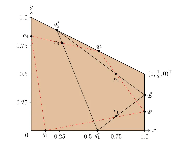
Lemma 4.1. Let R0 ⊆ P0 be the polygon with vertices r1, r2, r3 (see Figure 3). Write q1 = (u,0,0)>, where 0≤u≤1. If the supporting polygon Sq1 nested betweenR0 and P0 has
three vertices, then u≥2−√2.
x y
0.25 0.5 0.75 1.0 0.25
0.5 0.75 1.0
0
(1,12,0)>
r1 r2 r3
q1∗
q3∗ q2∗
q1
q3 q2
[image:10.612.128.445.90.339.2]q4
Figure 3. The outer polygon isP0 (after identifying the xy-plane inR3 withR2). The triangle with solid boundary is the supporting polygonSq∗
1, whereq ∗
1= (2− √
2,0,0)>. The quadrilateral with dashed boundary is the supporting polygonSq1 forq1= (
1 8,0,0)
>
.
Proof. Assume that Sq1 has three vertices and that 0≤ u≤ 2−√2. It suffices to show that these assumptions imply u = 2−√2. Moving counterclockwise, let the vertices of Sq1
be q1, q3, and q2. It follows by elementary geometry that (i) the line segment q1q3 passes throughr1andq3 lies on the right edge ofP0, and (ii) the line segment q3q2 passes throughr2
and q2 lies on the upper edge of P0. Figure 3shows the situations u= 2− √
2 and u= 18. Writing q3 = (1,v2,0)> and q2 = (1−w,12 + w2,0)>, where 0≤v, w ≤1, the collinearity conditions (i) and (ii) entail (see section 2.2)
u 0 1
1 v2 1
3 4
1 8 1
= 1 2uv−
1 8u−
3 8v+
1
8 = 0 and (7)
1 v2 1 1−w 12 +w2 1
3 4
1 2 1
= 1 2vw−
1 8v−
3 8w+
1
8 = 0. (8)
The assumption thatSq1 is the triangle4q1q3q2 entails that verticesq2, q1, r3 are in
counter-clockwise order. This implies
1−w 12 +w2 1
u 0 1
3 11
17 22 1
=−1
2wu+ 10 11w+
3 11u−
7
11 ≥0. (9)
x z
0.25 0.5 0.75 1.0 1.25 1.5 1.75 2.0 2.25 0.25
0.5 0.75 1.0 1.25
0
(94,0,12)> (0,0,87)>
r4 r5
r6
q∗1 q1
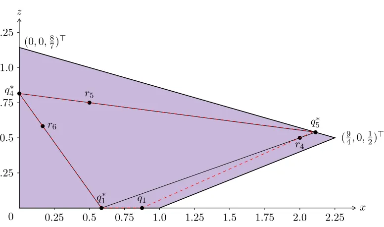
[image:11.612.102.490.90.319.2]q5∗ q4∗
Figure 4. The outer polygon isP1 (after identifying the xz-plane inR3 withR2). The triangle with solid boundary is the supporting polygonSq∗
1, whereq ∗
1= (2− √
2,0,0)>. The quadrilateral with dashed boundary is the supporting polygonSq1 forq1= (
7 8,0,0)
>
.
We use (7) and (8) to eliminate variables v, wfrom inequality (9), obtaining
15
22(8u−5)·(u
2−4u+ 2)≥0.
The only solution with 0≤u≤2−√2 isu= 2−√2. Let us writeV1⊆R6 for the affine span of M
:,4, M:,5, M:,6. We can also characterize V1 as
the image of the xz-plane in R3 under the map f :R3 →R6. Indeed, we have f(r4) = M:,4, f(r5) =M:,5, and f(r6) = M:,6. Thus the image of the xz-plane under f is a 2-dimensional
affine space that includes V1 and hence is equal to V1. Define the polygon P1 ⊆ R3 by P1 ={(x,0, z)> : (x,0, z)> ∈ P}. Then f restricts to a bijection betweenP1 and the set of
nonnegative vectors in V1. We have the following lemma.
Lemma 4.2. Let R1 ⊆ P1 be the polygon with vertices r4, r5, r6 (see Figure 4). Write q1 = (u,0,0)>, where 0≤u≤1. If the supporting polygon Sq1 nested betweenR1 and P1 has
three vertices, then u≤2−√2.
Proof. Assume that Sq1 has three vertices and that 2− √
2 ≤u ≤1. It suffices to show that these assumptions implyu= 2−√2. Moving counterclockwise, let the vertices ofSq1 be q1,q5, andq4. It follows by elementary geometry that (i) the line segmentq1q5passes through r4 and q5 lies on the upper edge of P1, and (ii) the line segment q5q4 passes through r5 and q4 lies on the left edge of P1. Figure 4shows the situations u= 2−
√
2 and u= 78.
Writingq5= (9−94v,0,7+914v)> and q4= (0,0,8−87w)>, where 0≤v, w≤1, the collinearity
conditions (i) and (ii) entail (see section 2.2)
u 0 1
9−9v
4
7+9v
14 1
2 12 1 = 9 14uv−
135 56 v+
1
8 = 0 and (10) 9−9v 4 7+9v 14 1
0 8−87w 1
1 2 3 4 1 = 18 7 vw−
9
16v−2w+ 9 16 = 0. (11)
The assumption thatSq1 is the triangle4q1q5q4 entails that verticesq4, q1, r6 are in
counter-clockwise order. This implies
0 8−87w 1
u 0 1
1 6 7 12 1 = 8 7wu−
4 21w−
47 84u+
4 21 ≥0. (12)
We use (10) and (11) to eliminate variablesv, w from the inequality (12), obtaining
−10
21(2u−7)·(u
2−4u+ 2) ≥0.
The only solution with 2−√2≤u≤1 isu= 2−√2.
4.2. Type 1. In this section we prove Proposition3.3(1), implying that any type-1 NMF of M requires irrational numbers (our argument will, in fact, depend only on the matrix M0
and not on Wε). Consider a type-1 NMF M =L·R, i.e., such that k= 1 and k1 =k2 = 2.
After a suitable permutation of its columns, Lmatches the pattern
L=
0 + + 0 0 0 0 0 + +
· · · · · · · · · · · · · · · · · · · · ,
where + denotes any strictly positive number. It follows from the zero pattern of M that
M:,1, M:,2, M:,3 all lie in the convex hull of L:,1, L:,2, L:,3, and M:,4, M:,5, M:,6 all lie in the
convex hull ofL:,1, L:,4, L:,5. Equivalently, there exist stochastic matricesR0, R1 ∈R3×3+ such
that
M:,1 M:,2 M:,3
= L:,1 L:,2 L:,3
·R0 and
(13)
M:,4 M:,5 M:,6
= L:,1 L:,4 L:,5
·R1.
Consider the polygon P0 ⊆R3 and the affine spaceV0 ⊆R6 from section 4.1. The affine
span of L:,1, L:,2, L:,3 includes V0 and has dimension at most 2, and hence is equal to V0. In
particular, L:,1, L:,2, L:,3 must all lie in V0. Since L:,1, L:,2, L:,3 are, moreover, nonnegative,
there are uniquely defined points q1, q2, q3 ∈ P0 such that f(qi) = L:,i for i ∈ {1,2,3}.
Applying the inverse of the map f columnwise to (13), we obtain
r1 r2 r3
= q1 q2 q3
·R0,
so the convex hull of q1, q2, q3 includes r1, r2, r3. In other words, triangle 4q1q2q3 is nested
between4r1r2r3 and polygon P0. SinceL:,1 has 0 in its first two coordinates, by inspecting
the definition of the mapf we see thatq1 = (u,0,0)>for someu∈R. By Lemma2.1it follows
that the supporting polygon Sq1 has three vertices. Hence Lemma 4.1impliesu≥2−√2. Considering the polygonP1 from section 4.1, we have q1 ∈ P1 (recall that f(q1) = L:,1).
Arguing as in the case ofP0, there are uniquely defined pointsq4, q5 ∈ P1such thatf(qi) =L:,i
fori∈ {4,5}. Similarly as before, triangle 4q1q4q5 is nested between 4r4r5r6 andP1. Then
Lemmas 2.1and 4.2imply u≤2−√2, and thusq1= (2−√2,0,0)>=q1∗. Hence
L:,1=f(q1) =f(q∗1) =W:,1.
Proposition3.3(1) follows.
We remark that this argument can be strengthened to show that any type-1 NMF of M
coincides with the one given in (2), up to a permutation of the columns of W and the rows of H0 Hε
; see AppendixA.
4.3. Type 2. In this section we exclude type-2 NMFs, i.e., we prove Proposition 3.3(2). Towards a contradiction, suppose there is a stochastic and at most 5-dimensional NMFM =
L·R with k= 2 and k1 = 1. Without loss of generality, the first three columns of L match
the following pattern:
L:,1 L:,2 L:,3
0 0 + 0 0 0
· · ·
· · ·
· · ·
· · ·
,
and the remaining columns have a strictly positive second coordinate. It follows from the zero pattern of M thatM:,1, M:,2, M:,3 all lie in the convex hull ofL:,1, L:,2, L:,3.
Consider again the polygon P0 ⊆ R3. For the purposes of the following argument, P0
is visualized on the left in Figure 5. Reasoning analogously to section 4.2, there are unique pointsq1, q2, q3 ∈ P0 withf(qi) =L:,ifori∈ {1,2,3}, and the convex hull ofq1, q2, q3 includes r1, r2, r3. Since L:,1 and L:,2 have 0 in their first two rows, inspecting the definition of the
map f, we see that q1 and q2 lie on the x-axis in R3. Thus, writing ˆq1 = (0,0,0)> and
ˆ
q2 = (1,0,0)>, triangle4qˆ1qˆ2q3 includes triangle 4q1q2q3 and hence also contains the points r1, r2, r3. But clearly there is no point q3 ∈ P0 such that 4q1ˆq2q3ˆ includes both r2 and r3
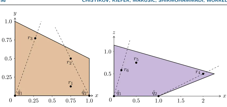
(see, e.g., Figure 5, left), which is a contradiction. Thus we have proved Proposition3.3(2).
x y
0.25 0.5 0.75 1.0 0.25
0.5 0.75 1.0
0
r1 r2 r3
ˆ
q1 qˆ2
x z
0.5 1.0 1.5 2 0.5
1.0
0
r4 r5
r6
ˆ
[image:14.612.76.509.77.281.2]q1 qˆ2
Figure 5. Left: there is no pointq3 in the quadrilateral P0 such that4qˆ1qˆ2q3 includes bothr2 and r3. Right: there is no pointq3 in the quadrilateralP1 such that4qˆ1qˆ2q3 includes bothr4 andr6.
4.4. Type 3. In this section we exclude type-3 NMFs, i.e., we prove Proposition 3.3(3). The reasoning is entirely analogous to section4.3. Towards a contradiction, suppose there is a stochastic and at most 5-dimensional NMF M = L·R with k = 2 and k2 = 1. Consider
again the polygon P1 ⊆R3. For the purposes of the following argument, P1 is visualized on
the right in Figure5. Analogously to section4.3, there are pointsq1, q2, q3 ∈ P1 whose convex
hull includesr4, r5, r6, andq1 andq2 lie on thex-axis inR3. Thus, writing ˆq1= (0,0,0)> and
ˆ
q2 = (1,0,0)>, triangle 4q1ˆq2q3ˆ includes the points r4, r5, r6. But clearly there is no point
q3 ∈ P1 such that 4qˆ1qˆ2q3 includes both r4 and r6 (see, e.g., Figure 5, right), which is a
contradiction. Thus we have proved Proposition 3.3(3).
4.5. Type 4. In this section we exclude type-4 NMFs, i.e., we prove Proposition 3.3(4). In fact, sections 4.2–4.4prove the stronger result that there is no rational NMF of types 1, 2, 3 for the matrix M0 alone. Here we spell out the role of Wε, effectively explaining why the
matrixM = M0 Wε
is defined the way it is.
Observe that adding toM0 new columns from the convex hull of the columns ofW shrinks the set of possible nonnegative factorizations. Given this, our goal is to find a matrix satisfying the following desiderata:
• its entries are rational,
• its columns belong to the convex hull of the columns ofW, and
• it has no type-4 NMF.
The first two items ensure that M, while being rational, admits a nonnegative factorization with left factorW, ensuring that the nonnegative rank ofM overRis (at most) 5. The third
condition, combined with the arguments from sections 4.2–4.4, ensures that the nonnegative rank ofM overQis 6.
While the matrixW manifestly fails the first desideratum, it satisfies the second and third as follows.
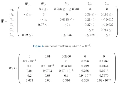
Claim 4.3. The matrixW and, therefore, the matrixM = M0 W
have no type-4 NMF.
f
W =
f
W:,1 Wf:,2 Wf:,3 fW:,4 Wf:,5
f
W1,: 0 0.8≤ · 0.286≤ · ≤0.287 0 0
f
W2,: · ≤ε 0 0 0.29≤ · 0.196≤ ·
f
W3,: · ≤ε 0.0335≤ · 0.21≤ · · ≤0.015
f
W4,: 0.07≤ · · ≤ε 0.27≤ · · ≤0.022
f
W5,: · ≤ε 0.767≤ ·
f
W6,: 0.62≤ · · ≤0.32 · ≤0.21 · ≤ε
[image:15.612.82.487.104.397.2]
Figure 6. Entrywise constraints, whereε= 10−5.
0 0.81 0.2866 0 0 0.9·10−5 0 0 0.296 0.1962
0.1 0.7·10−5 0.03360 0.219 0.0144 0.04 0.0703 0.97·10−5 0.276 0.0216 0.2 0.08 0.4 0.9·10−5 0.7679 0.621 0.04 0.316 0.208 0.98·10−5
Wε≈
Figure 7. Matrix Wε with entries rounded off.
This reasoning motivates the main technical result of this section, which is a strengthening of Claim4.3 showing that no matrix in a suitably small neighborhood ofW admits a type-4 NMF.
Lemma 4.4. For all stochastic matrices Wf ∈ R6×5+ satisfying the entrywise constraints given in Figure 6, there exists no type-4 NMFWf=L·R.
In particular, the constraints of Lemma 4.4, and in fact all three desiderata, are satisfied by the matrixWε from Theorem3.1; see Figure7. Therefore, the matrixM = M0 Wε
has no type-4 NMF, thus concluding the proof of Proposition 3.3(4).
Remark 4.5. The existence of a suitable matrixWε can be understood in terms of upper
semicontinuity of the nonnegative rank over the reals [4] and can be alternatively demon-strated using a nonconstructive argument that assumes only Claim4.3instead of the (stronger) Lemma 4.4; see Appendix B for details. We are not, however, aware of a simpler proof of Claim4.3.
Proof of Lemma4.4. The idea of the proof is to derive a contradiction from the assump-tion that there exists a stochastic matrixWf∈R6×5+ that satisfies the constraints in Figure6
and has an NMFWf=L·R of type 4, i.e., such that Lmatches the following zero pattern:
L=
+ 0 0 0 0 0 + 0 0 0
· · · · ·
· · · · ·
· · · · ·
· · · · ·
.
To this end, we use constraint propagation to successively derive lower and upper bounds for various entries of the matrices Land R until we reach a contradiction.
In our proof of the lemma, we use the following two assumptions, which are without loss of generality:
(A1) L6,3 = max{L6,3, L6,4, L6,5},and
(A2) L5,4 = max{L5,4, L5,5}.
Technically, these assumptions are used only in the proof of Claim4.6 below. We first demonstrate that Lemma 4.4follows from the following two claims. Claim 4.6. L6,3 ≥0.61, L5,4 ≥0.9539.
Claim 4.7. L4,3 ≥0.346, max{L3,3, L3,4} ≥0.0465.
Proof of Lemma 4.4. Take the second inequality of Claim4.7and consider two cases:
• First, suppose that in Claim 4.7 it holds that max{L3,3, L3,4} = L3,3. Then L3,3 ≥
0.0465. Further, Claims 4.7 and 4.6 give lower bounds on L4,3 and L6,3, respectively. Since
the elements of each column of L sum up to 1, it follows that 0.0465 + 0.346 + 0.61 ≤ L3,3+L4,3+L6,3 ≤1. This is a contradiction.
• Otherwise, we have max{L3,3, L3,4} = L3,4 ≥ 0.0465. Recall that Claim 4.6 gives L5,4 ≥0.9539. Hence 0.0465 + 0.9539≤L3,4+L5,4≤1, which is also a contradiction.
Our two goals now are to prove Claims4.6and 4.7. We achieve these using a sequence of auxiliary statements.
Claim 4.8. 0.29≤R2,4,0.196≤R2,5.
Proof. Observe that all columns of fW lie in the convex hull of columns ofL sinceW:f,j =
L·R:,j. Consider the fourth and fifth columns Wf:,4,Wf:,5. Since L:,2 is the only column of L with strictly positive second component, we have Wf2,4 = L2,2·R2,4 and Wf2,5 = L2,2 ·R2,5. Therefore,
0.29≤Wf2,4=L2,2·R2,4 ≤R2,4, 0.196≤fW2,5=L2,2·R2,5 ≤R2,5,
implying the claim.
By omitting nonnegative terms from the equalityfWi,j =Li,:·R:,j, we obtain the inequality
Li,k·Rk,j≤fWi,j, which holds for all 1≤k≤5. We can thus compute an upper bound onLi,k (resp., onRk,j) if we know a lower bound onRk,j(resp., onLi,k). We refer to this as computing
simple upper bounds through fWi,j.
Henceforth, we set ε= 10−5, as in Figure6.
Claim 4.9. The matrix L satisfies the following constraints:
L:,1 L:,2 L:,3 L:,4 L:,5
L1,:
L2,: 0.8≤ ·
L3,: · ≤0.077
L4,: · ≤0.12
L5,: · ≤4ε
L6,: · ≤6ε
.
Proof. First, note that, by Claim 4.8, 0.196 ≤ R2,5. This lets us derive the following
simple upper bounds through fW3,5,Wf4,5, and fW6,5:
L3,2 ≤
0.015
0.196 ≤0.077, L4,2 ≤ 0.022
0.196 ≤0.12, L6,2 ≤
ε
0.196 ≤6ε.
The remaining bounds are obtained as follows. The lower bound onR2,4, taken from Claim4.8,
gives a simple upper boundL5,2 ≤ε/0.29≤4εthroughWf5,4. Now the upper bounds onLi,2, where 3≤i≤6, result in the inequality L2,2≥1−(0.077 + 0.12 + 10ε)≥0.8.
Now we are able to prove Claim 4.6.
Proof of Claim 4.6. We use the bounds of Claim4.9and the inequalitiesfW2,1≤ε,fW6,1 ≥ 0.62, andWf5,5 ≥0.767 from the statement of Lemma 4.4.
To begin with, the first column ofWflies in the convex hull ofL:,2 andL:,3, L:,4, L:,5. From
the lower bound L2,2≥0.8 we compute the simple upper bound R2,1 ≤2εthrough fW2,1. By our assumption (A1),L:,3 has the largest sixth coordinate amongL:,3, L:,4, and L:,5, so from
0.62≤W6f,1=L6,:·R:,1 ≤L6,2·R2,1+ (1−R2,1)·L6,3≤L6,2·R2,1+L6,3
we obtainL6,3 ≥0.62−6ε·2ε≥0.61, as claimed.
Furthermore, the fifth column ofWf also lies in the convex hull of L:,2 and L:,3, L:,4, L:,5. Recall that L5,2 is at most 4ε, and R2,5 is at least 0.196 by Claim 4.8. We then have
0.767≤Wf5,5=L5,:·R:,5 ≤L5,2+ (1−R2,5)·max{L5,3, L5,4, L5,5},
yielding the bound max{L5,3, L5,4, L5,5} ≥ 01−0.767−4.196ε ≥ 0.9539. As we already know that L6,3 ≥0.61, we deduce that the maximum in the left-hand side cannot be attained by L5,3,
since the column vectorL:,3 is stochastic. Now, by our assumption (A2)we must haveL5,4 ≥
0.9539.
Our next goal is prove Claim4.7. Claim 4.10 and Claim 4.11, described below, take two consecutive steps in this direction.
Claim 4.10. R5,2≤50ε,R5,3≤23ε.
Proof. First, note that the matrix L satisfies the following constraints:
(14)
L:,1 L:,2 L:,3 L:,4 L:,5
L1,:
L2,:
L3,: · ≤0.077 · ≤0.0461
L4,: · ≤0.12 · ≤0.0461
L5,: 0.9539≤ ·
L6,: 0.61≤ ·
.
Indeed, the upper bounds onL3,2 andL4,2 are taken verbatim from Claim4.9, and the lower
bounds on L6,3 and L5,4 from Claim 4.6. The latter bound implies the upper bounds onL3,4
and L4,4.
We first prove the inequality R5,2 ≤ 50ε. By multiplying the row vector
0 0 2 0 0 −1 with W:f,4 = L ·R:,4, we obtain 2W3f,4 −fW6,4 = (2L3,:−L6,:) ·R:,4. Since the fourth column ofWf lies in the convex hull ofL:,2 and L:,3, L:,4, L:,5, we also have
2fW3,4−W6f,4 ≤max{2L3,2−L6,2, 2L3,3−L6,3, 2L3,4−L6,4, 2L3,5−L6,5}
≤max{2L3,2−L6,2, 2L3,3−L6,3, 2L3,4−L6,4}+ 2L3,5.
On the one hand, we have 2fW3,4−W6f,4 ≥0.21, because W3f,4 ≥0.21 and W6f,4 ≤0.21. On the other hand, 2L3,3−L6,3≤2 (1−L6,3)−L6,3= 2−3L6,3. Hence
0.21≤max{ 2L3,2
| {z }
≤2·0.077
,2−3L6,3
| {z }
≤2−3·0.61
, 2L3,4
| {z }
≤2·0.0461
}+ 2L3,5,
where the inequalities are taken from (14) and from the calculation above. Therefore,L3,5 ≥
0.02, from which we derive the simple upper boundR5,2≤50εthrough W3f,2.
The second inequality, R5,3 ≤ 23ε, is proved in a similar way. By multiplying the row
vector 0 0 0 2 0 −1withW:f,4=L·R:,4, we obtain 2W4f,4−fW6,4 = (2L4,:−L6,:)·R:,4 and thus
2fW4,4−W6f,4 ≤max{2L4,2−L6,2, 2L4,3−L6,3, 2L4,4−L6,4}+ 2L4,5.
On the one hand, we have 2fW4,4 −W6f,4 ≥ 2 ·0.27 −0.21 ≥ 0.33. On the other hand, 2L4,3−L6,3 ≤2(1−L6,3)−L6,3 = 2−3L6,3. Hence
0.33≤max{2L4,2
| {z }
≤2·0.12
,2−3L6,3
| {z }
≤2−3·0.61
, 2L4,4
| {z }
≤2·0.0461
}+ 2L4,5 ,
where the inequalities are again taken from (14) and from the calculation above. It follows thatL4,5 ≥0.045, and we derive the simple upper boundR5,3≤ε/0.045≤23εthroughW4f,3. This completes the proof.
Claim 4.11. The matrices L andR satisfy the following constraints:
L:,1 L:,2 L:,3 L:,4 L:,5
L1,:
L2,:
L3,: · ≤2ε
L4,: · ≤4ε · ≤10ε
L5,:
L6,:
R:,1 R:,2 R:,3 R:,4 R:,5
R1,: 0.8≤ · 0.286≤ ·
R2,:
R3,:
R4,:
R5,: · ≤50ε · ≤23ε
.
Proof. First, note that the constraints R5,2 ≤ 50ε and R5,3 ≤23ε are already known to
us from Claim 4.10. We now show how to obtain the remaining five constraints.
Observe that the columnL:,1 is the only column ofL that has a positive first component;
hence it is the only column ofLthat contributes to the positive first component in the second and third columns ofWf. Therefore, the following inequalities indeed hold:
0.286≤W1f,3=L1,1·R1,3 ≤R1,3 and 0.8≤Wf1,2=L1,1·R1,2 ≤R1,2.
The latter inequality leads to the claimed simple upper boundL3,1 ≤ε/0.8≤2εthroughW3f,2. We further derive the following simple upper bounds:
• R1,3 ≤ 0.287/0.8 ≤ 0.36 through Wf1,3, since L1,1 ≥ L1,1 ·R1,2 = Wf1,2 ≥ 0.8 by the above;
• R3,3 ≤0.32/0.61≤0.53 throughWf6,3, sinceL6,3 ≥0.61 by Claim4.6.
Since W:f,3 lies in the convex hull of L:,1 and L:,3, L:,4, L:,5, we can deduce that R4,3 = 1−
R1,3 −R3,3−R5,3 ≥ 1−0.36−0.53−23ε ≥ 0.1. Using this lower bound, R4,3 ≥ 0.1, and
the lower boundR1,3 ≥0.286 obtained above, we deduce, throughW4f,3, simple upper bounds
L4,4 ≤10εand L4,1 ≤4ε. This concludes the proof.
We are now ready to prove Claim 4.7.
Proof of Claim 4.7. Here we will use only the result of Claim4.11.
First, note that the second column of fW lies in the convex hull ofL:,1,L:,3,L:,4, andL:,5. We have
0.07≤fW4,2 =L4,:·R:,2=L4,1R1,2+L4,3R3,2+L4,4R4,2+L4,5R5,2
≤L4,1
|{z}
≤4ε
+L4,3(1−R1,2)
| {z }
≤0.2
+L4,4
|{z}
≤10ε
+R5,2
|{z}
≤50ε
,
which gives us the lower bound 0.346≤L4,3.
Similarly, consider the third column of fW and observe that
0.0335≤W3f,3 =L3,:·R:,3=L3,1R1,3+L3,3R3,3+L3,4R4,3+L3,5R5,3
≤L3,1
|{z}
≤2ε
+ max{L3,3, L3,4}(1−R1,3)
| {z }
≤0.714
+R5,3
|{z}
≤23ε
.
The lower bound max{L3,3, L3,4} ≥0.0465 follows.
As we have seen above, Lemma 4.4follows from Claims4.6 and4.7.
5. Conclusions. In this paper we have solved the Cohen–Rothblum problem, showing that nonnegative ranks over R and over Q may differ. More precisely, our construction applies
to matrices of rank 4 and higher. It was already known to Cohen and Rothblum [9] that nonnegative ranks overRandQcoincide for matrices of rank at most 2, and Kubjas, Robevas,
and Sturmfels [16] showed that this also holds for matrices of nonnegative rank (overR) at
most 3. The remaining open question is whether nonnegative ranks over Rand over Qdiffer
for rank-3 matrices whose nonnegative rank (overR) is at least 4—or whether our example is
optimal in this sense.
As our results show that the nonnegative ranks overRand Qare different functions, the
computability question emerges. It has long been known (see, e.g., Cohen and Rothblum [9]) that the nonnegative rank overR is computable, via a reduction to the existential theory of
the reals, which in turn can be decided inPSPACE. (Recently, Shitov proposed a reduction in the converse direction, i.e., from the existential theory of the reals to NMF [24].) In contrast, it is not known whether the nonnegative rank over Qis computable. While there is a natural
reduction to the decision problem for the existential theory of the rationals, the decidability of the latter is a long-standing and very prominent open question [21].
Finally, we would like to point out that the complexity of the following geometric problem closely linked to NMF, the nested polytope problem, is not fully known. This problem asks, given an ordered fieldFand polytopesS ⊆ T inFn, whether there exists asimple polytopeN
such that S ⊆ N ⊆ T (cf. Gillis and Glineur [14]). The definition of “simple” can be either “having at most k vertices,” or “having at most k facets,” or a combination of both. For
F = R, minimizing the number of vertices or, dually, facets is known to require irrational
numbers [7] even in the case of full-dimensional S. While for some representations of the polytopes such questions are known to be NP-hard (see, e.g., Das and Goodrich [10]), their precise complexity is not known in general.
Appendix A. Uniqueness of type-1 NMFs of M. In this appendix, we strengthen
Proposition3.3(1) to show that any type-1 NMF of M coincides with the one given in equa-tion (2), up to a permutaequa-tion of the columns of W and the rows of H0 Hε
. Together with the other parts of Proposition 3.3, this implies that the NMF (2) is the only 5-dimensional stochastic NMF of the matrixM, up to permutations.
Proposition A.1. If M =L·R is a type-1NMF, thenL is equal toW up to a permutation of its columns.
Proof. We recall from Figure 3 that the supporting polygon Sq∗
1, nested between the
triangle4r1r2r3 and the polygonP0, is the triangle4q∗1q∗3q∗2. Similarly, as seen in Figure 4,
the supporting polygon Sq∗
1, nested between the triangle 4r4r5r6 and the polygonP1, is the
triangle4q1∗q5∗q4∗. We have already shown thatq1 =q1∗. In the following, we show thatqi =q∗i
for each i∈ {2,3,4,5}.
Towards a contradiction, suppose that q2 6= q2∗ or q3 6= q∗3. Let us consider the case
whenq26=q∗2. Observe that triangles 4q∗1q3∗q∗2 and 4q1∗q3q2 are both nested between4r1r2r3
and P0. The fact that 4r1r2r3 ⊆ 4q1∗q3q2 implies that vertices q3 and q2 lie to the right
of (or on) directed line segments q∗1q∗3 and q∗2q∗1, respectively. Since, moreover, q3, q2 ∈ P0,
it holds that vertex q3 lies to the left of (or on) directed line segment q3∗q2∗, whereas vertex q2 lies strictly to the left of q3∗q2∗. However, this implies that the point r2 is to the right of directed line segment q3q2, which contradicts the assumption that4r1r2r3 ⊆ 4q1∗q3q2. The
case q3 6= q3∗ analogously leads to a contradiction. We conclude that q2 = q2∗ and q3 = q3∗.
Analogously, using Lemma4.2 one can show thatq4 =q4∗ and q5 =q∗5.
Since f(qi) =L:,i andf(q∗i) =W:,i for eachi∈ {2,3,4,5}, we conclude that{L:,2, L:,3}= {W:,2, W:,3}and{L:,4, L:,5}={W:,4, W:,5}. Therefore, the NMFM =L·Rcoincides with the
one given in (2), up to a permutation of the columns of W and the rows of H0 Hε
.
Appendix B. A nonconstructive approach to defining Wε. Instead of deducing the
result of section4.5from Lemma4.4, one can alternatively rely on its weaker form, Claim4.3, and give a nonconstructive proof of the existence of an appropriateWε (satisfying the three
desiderata given as bullet points in section 4.5 on page298) via a topological argument that we sketch below. However, we emphasize that we do not know how to prove Claim4.3without following the arguments that prove Lemma 4.4.
Proposition B.1. There exists a 6×5 matrix such that
• its entries are rational,
• its columns belong to the convex hull of the columns of W, and
• it has no type-4 NMF.
Proof. We first employ the geometric constructions of section 4.1 to argue that every neighborhood of the matrixW contains a rational matrix that factors throughW, i.e., whose columns belong to the convex hull of the columns of W. Indeed, consider the set F of all stochastic real matrices of size 6×5 that have a stochastic NMF with left factorW. Observe that F can be characterized as the set of matrices whose columns lie in the image under f
of a full-dimensional set in R3, namely of the convex hull of q∗1, . . . , q5∗. Since the map f is
specified by matrices C and d with rational coefficients, it immediately follows that the set of rational matrices is dense in F. As every δ-neighborhood of the matrix W includes some 3-dimensional subset of F, it also contains a rational matrix Wδ from F, as we wished to
prove.
Now assume for the sake of contradiction that every rational matrix in the set F has a type-4 NMF. Then the matrices Wδ from above also have type-4 NMFs Wδ = Lδ·Rδ for
all δ > 0. By compactness, there exists a subsequence of matrices Wδ with decreasing δ
such that the corresponding sequences Lδ and Rδ converge. Taking the limit, we arrive at
the equality W =L·R, where the right-hand side is also a type-4 NMF—which contradicts Claim 4.3. This completes the proof. (Note that Lemma4.4 contains a constructive version of this argument.)
It is worth mentioning that this reasoning follows similar lines as the upper semicontinu-ity argument for nonnegative rank [4]: the nonnegative rank of any (rational or irrational) matrix Wε which is entrywise close enough to W can only be greater than or equal to that
of W.
Acknowledgments. The authors would like to thank Vladimir Lysikov and Vladimir
Shiryaev for stimulating discussions.
REFERENCES
[1] A. Aggarwal, H. Booth, J. O’Rourke, S. Suri, and C. K. Yap, Finding minimal convex nested polygons, Inform. and Comput., 83 (1989), pp. 98–110.
[2] S. Arora, R. Ge, R. Kannan, and A. Moitra, Computing a nonnegative matrix factorization— provably, SIAM J. Comput., 45 (2016), pp. 1582–1611,https://doi.org/10.1137/130913869.
[3] S. Arora, R. Ge, and A. Moitra, Learning topic models—going beyond SVD, in Proceedings of the 53rd Annual IEEE Symposium on Foundations of Computer Science (FOCS), New Brunswick, NJ, 2012, pp. 1–10.
[4] C. Bocci, E. Carlini, and F. Rapallo,Perturbation of matrices and nonnegative rank with a view toward statistical models, SIAM J. Matrix Anal. Appl., 32 (2011), pp. 1500–1512,https://doi.org/10. 1137/110825455.
[5] J. Canny,Some algebraic and geometric computations in PSPACE, in Proceedings of the 20th Annual ACM Symposium on Theory of Computing (STOC), ACM, New York, 1988, pp. 460–467.
[6] D. Chistikov, S. Kiefer, I. Maruˇsi´c, M. Shirmohammadi, and J. Worrell, Nonnegative Matrix Factorization Requires Irrationality, preprint,https://arxiv.org/abs/1605.06848, 2016.
[7] D. Chistikov, S. Kiefer, I. Maruˇsi´c, M. Shirmohammadi, and J. Worrell,On restricted nonneg-ative matrix factorization, in Proceedings of the 43rd International Colloquium on Automata, Lan-guages and Programming (ICALP ’16), Schloss Dagstuhl–Leibniz-Zentrum fuer Informatik, Dagstuhl, Germany, 2016, pp. 103:1–103:14.
[8] D. Chistikov, S. Kiefer, I. Maruˇsi´c, M. Shirmohammadi, and J. Worrell, On rationality of nonnegative matrix factorization, in Proceedings of the Twenty-Eighth Annual ACM-SIAM Sympo-sium on Discrete Algorithms (SODA), ACM, New York, SIAM, Philadelphia, 2017, pp. 1290–1305,
https://doi.org/10.1137/1.9781611974782.84.
[9] J. E. Cohen and U. G. Rothblum,Nonnegative ranks, decompositions, and factorizations of nonnega-tive matrices, Linear Algebra Appl., 190 (1993), pp. 149–168.
[10] G. Das and M. T. Goodrich,On the complexity of approximating and illuminating three-dimensional convex polyhedra, in Algorithms and Data Structures: 4th International Workshop (WADS), Springer, Berlin, Heidelberg, 1995, pp. 74–85.
[11] R. Eggermont, E. Horobet, and K. Kubjas,Algebraic boundary of matrices of nonnegative rank at most three, Linear Algebra Appl., 508 (2016), pp. 62–80.
[12] N. Gillis,Sparse and unique nonnegative matrix factorization through data preprocessing, J. Mach. Learn. Res., 13 (2012), pp. 3349–3386.
[13] N. Gillis,The why and how of nonnegative matrix factorization, in Regularization, Optimization, Ker-nels, and Support Vector Machines, J. Suykens, M. Signoretto, and A. Argyriou, eds., Machine Learning and Pattern Recognition Series, Chapman & Hall/CRC, Boca Raton, FL, 2014, pp. 257– 291. Preprint version available athttps://arxiv.org/abs/1401.5226.
[14] N. Gillis and F. Glineur, On the geometric interpretation of the nonnegative rank, Linear Algebra Appl., 437 (2012), pp. 2685–2712.
[15] D. A. Gregory and N. Pullman,Semiring rank: Boolean rank and nonnegative rank factorizations, J. Combin. Inform. System Sci., 8 (1983), pp. 223–233.
[16] K. Kubjas, E. Robeva, and B. Sturmfels,Fixed points of the EM algorithm and nonnegative rank boundaries, Ann. Statist., 43 (2015), pp. 422–461.
[17] H. Laurberg, M. G. Christensen, M. D. Plumbley, L. K. Hansen, and S. H. Jensen,Theorems on positive data: On the uniqueness of NMF, Comput. Intell. Neurosci., 2008 (2008), 764206. [18] W. H. Lawton and E. A. Sylvestre,Self modeling curve resolution, Technometrics, 13 (1971), pp. 617–
633.
[19] A. Moitra,An almost optimal algorithm for computing nonnegative rank, SIAM J. Comput., 45 (2016), pp. 156–173,https://doi.org/10.1137/140990139.
[20] D. Mond, J. Smith, and D. van Straten, Stochastic factorizations, sandwiched simplices and the topology of the space of explanations, Proc. R. Soc. Lond. A, 459 (2003), pp. 2821–2845.
[21] B. Poonen,Hilbert’s Tenth Problem over Rings of Number-Theoretic Interest, Note from the lecture at the Arizona Winter School on “Number Theory and Logic,” 2003,http://math.mit.edu/∼poonen/
papers/aws2003.pdf.
[22] Y. Shitov,Nonnegative Rank Depends on the Field, preprint,https://arxiv.org/abs/1505.01893, 2015. [23] Y. Shitov,Nonnegative Rank Depends on the FieldII, preprint,https://arxiv.org/abs/1605.07173, 2016. [24] Y. Shitov,A Universality Theorem for Nonnegative Matrix Factorizations, preprint,https://arxiv.org/
abs/1606.09068, 2016.
[25] D. Simanek,How to View3D Without Glasses,https://www.lhup.edu/∼dsimanek/3d/view3d.htm. (Ac-cessed May 19, 2017.)
[26] L. B. Thomas, Rank factorization of nonnegative matrices (A. Berman and R. J. Plemmons), SIAM Rev., 16 (1974), pp. 393–394,https://doi.org/10.1137/1016064.
[27] S. A. Vavasis, On the complexity of nonnegative matrix factorization, SIAM J. Optim., 20 (2009), pp. 1364–1377,https://doi.org/10.1137/070709967.
[28] S. Venkatasubramanian,Computational geometry column55: New developments in nonnegative matrix factorization, SIGACT News, 44 (2013), pp. 70–78.
[29] M. Yannakakis,Expressing combinatorial optimization problems by linear programs, J. Comput. Syst. Sci., 43 (1991), pp. 441–466.
[30] S. Kiefer, NMF Computations, http://www.cs.ox.ac.uk/people/stefan.kiefer/NMFcomputations.html
(accessed May 19, 2017).