For Peer Review
Coverage Performance in Multi-Stream
MIMO-ZFBF Heterogeneous Networks
Mohammad G. Khoshkholgh, Kang G. Shin, Life Fellow, IEEE,
Keivan Navaie, Senior Member, IEEE, Victor C. M. Leung, Fellow, IEEE
Abstract— We study the coverage performance of multi-antenna (MIMO) communications in heterogenous networks (HetNets). Our main focus is on open-loop and multi-stream MIMO zero-forcing beamforming (ZFBF) at the receiver. Net-work coverage is evaluated adopting tools from stochastic ge-ometry. Besides fixed-rate transmission (FRT), we also consider adaptive-rate transmission (ART) while its coverage perfor-mance, despite its high relevance, has so far been overlooked. On the other hand, while the focus of the existing literature has solely been on the evaluation of coverage probability per stream, we target coverage probability per communication link — comprising multiple streams — which is shown to be a more conclusive performance metric in multi-stream MIMO systems. This, however, renders various analytical complexities rooted in statistical dependency among streams in each link. Using a rigorous analysis, we provide closed-form bounds on the coverage performance for FRT and ART. These bounds explicitly capture impacts of various system parameters including densities of BSs, SIR thresholds, and multiplexing gains. Our analytical results are further shown to cover popular closed-loop MIMO systems, such as eigen-beamforming and space-division multiple access (SDMA). The accuracy of our analysis is confirmed by extensive simulations. The findings in this paper shed light on several important aspects of dense MIMO HetNets: (i) increasing the multiplexing gains yields lower coverage performance; (ii) densifying network by installing an excessive number of low-power femto BSs allows the growth of the multiplexing gain of high-power, low-density macro BSs without compromising the coverage performance; and (iii) for dense HetNets, the coverage probability does not increase with the increase of deployment densities.
Index Terms— Coverage probability, densification, Heteroge-nous Cellular Networks (HetNets), Input Multiple-Output (MIMO) systems, stochastic geometry, Poisson point process, Zero-Forcing Beamforming.
I. INTRODUCTION
Multi-Input Multi-Output (MIMO) communication is a promising technology due to its potential of achieving high spectral efficiency and reliability often without requiring high transmission power [1]. Supported by decades of thorough investigations, MIMO communications have thus far been embodied in multiple IEEE 802.11 standards as well as 3GPP LTE-Advanced [2]. To cope with the rapid growth of wireless
Manuscript received April 29, 2016, revised September 13, 2016. M. G. Khoshkholgh and V. C. M. Leung ([email protected], [email protected]) are with the Department of Electrical and Computer Engineering, the University of British Columbia, Vancouver, BC, Canada V6T 1Z4 ; K. G. Shin ([email protected]) is with the Department of Electrical Engineering and Computer Science, University of Michigan, Ann Arbor, MI 48109-2121, U.S.A.; K. Navaie ([email protected]) is with School of Computing and Communications, Lancaster University, Bailrigg Lancaster LA1 4WA United Kingdom.
traffic demand [3], MIMO technologies have been re-emerging through copious innovative ideas. Thus, pervasive exploita-tions of sophisticated MIMO technologies in conjunction with unprecedented densification in heterogeneous networks (HetNets) are envisioned as the main design paradigm in next-generation cellular communication systems [4], [5].
There has been extensive research on the application of MIMO in HetNets, mainly focusing on isolated scenarios (e.g., [6]); for example, by evaluating the performance of femto-cells overlaying/underlaying macro-cells. This line of research, however, falls short of characterizing the network-wise performance of MIMO in HetNets. Network-network-wise perfor-mance is of utmost importance when it comes to design and implementation of large-scale communication systems with millions of nodes. This shortcoming is rooted in the simplified and often unrealistic assumptions made on the incorporation of inter-cell interference (ICI) in system analysis. As a result, while in a single cell system, allocating the system resources is rather straightforward, the same cannot be directly applied in the network-wise performance context. For instance, in a single cell system, decisions such as the number of antennas to be switched on/off, the number of user equipments (UEs) to be concurrently served, or choosing between multiplexing (using antennas for increasing data rate) and diversity (using antennas for increasing reliability) are easy to make [1], [7], whereas in a multi-cell network, such decisions need sophisticated solutions incorporating the inter-cell impact based on network-wise performance metrics. While increasing the number of transmitted data streams (i.e., increasing the multiplexing gain) in a single-cell system is (locally) optimal, it increases the ICI, almost with the same order, which could offset the effect of the former. It is, therefore, debatable whether strategies yielding higher capacity or better coverage from the perspective of local decisions (isolated scenarios) result in network-wise optimality.
One approach to capturing the network-wise effects of adopting MIMO is to employ analytical tools from stochastic geometry, see, e.g., [8], [9] and references therein. Such techniques are widely used in modeling and analyzing ad hoc and sensor networks, [10], [11], [12], and recently cellular communications [13]. Some researchers, however, have casted skepticism on the accuracy of Poisson Point Process (PPP) for modeling the locations of macro BSs [14]. This is because PPP models position the BSs in the network plane almost indis-criminately, whereas in practice, macro BSs are often placed far from each other. This issue is investigated further in [13], where the PPP assumption is shown to result in adequately
For Peer Review
precise characterization of macro BSs, and in fact, provides a rather pessimistic bound on the coverage performance in contrast to other analytic methods such as hexagonal and lattice models, see, e.g., [15] that provide optimistic bounds. The PPP models have also been widely used for modeling and analyzing HetNets, e.g., [16], [17], [18]. The pioneering work of [16] proposed a flexible approach in modelingK-tier HetNets1 throughK tiers of independent PPPs.
In this paper, we extend the approach in [16] to multi-stream MIMO HetNets and investigate their coverage per-formance. Our focus is on open-loop MIMO zero-forcing beamforming (MIMO-ZFBF), which is practically attractive due to its straightforward implementation, low computational complexity, and almost zero feedback overhead. The network-wise performance of MIMO-ZFBF, as well as other pertinent MIMO techniques, is nevertheless extensively studied in the context of ad hoc networks, see, e.g., [19], [20], [21], [22], [23], [24]. The work of [20] is practically relevant to this paper as their focus is also on open loop MIMO such as ZFBF. Several advantages of ZFBF in enhancing the coverage performance of ad hoc networks were highlighted there, and multi-stream communications were proven to outperform ideal single-stream ad hoc networks for practical settings.
In light of the above findings in the context of ad hoc networks, one may argue that the same trends can hold in MIMO HetNets by noticing the convergence, albeit partial, of HetNets toward ad hoc networks, for instance through random installation of remote antenna ports, relays, and small cells. Apart from such analogies, there exist significant discrepancies between these two networks due mainly to the corresponding CA mechanisms governing HetNets, as well as centralized TDMA/FDMA MAC protocols.
It is, therefore, necessary to investigate whether or not
multi-stream MIMO schemes are of practical significance in enhancing the coverage performance of HetNets? It is equally
important to understand whether in MIMO HetNets, cell
densification and high multiplexing gains should be practiced simultaneously in all tiers? If not, new techniques are needed to evaluate whether for a given setting excessive densification is preferable to increasing multiplexing gains?
Despite significant progress in analyzing MIMO commu-nications in HetNets, the existing results are inadequate to comprehensively address the above concerns and other similar questions. To address this inadequacy, we derive closed-form bounds on the the coverage performance of MIMO communi-cations. The thus-obtained analytical results enable thorough investigation of densification and multiplexing gains in MIMO HetNets.
A. Related Work
The authors of [25] considered MIMO-based HetNets where a single macro-cell system overlaid by a number of multi-antenna femto cells was investigated. The system in [25] adopts spatial division multiple access (SDMA) beamforming and in each cell, a number of UEs, each with a single antenna, are served. For this configuration, the authors of [25] show that
1K-tier HetNets consist ofKspatially and spectrally coexisting tiers, each
with its own BS.
the system achieves a higher area spectral efficiency by solely serving one UE per femto-cell via conventional beamforming. The results in [25] are extended in [26] toK-tier multi-input single-output (MISO) HetNets, under the assumption of max-imum SIR CA rule. By comparing the coverage probability, the authors of [26] showed that spatial division multiple access (SDMA) is inferior to the schemes which support one UE per cell. This conclusion is also confirmed in [27] for a clustered ad hoc network with quantized beamforming.
Area spectral efficiency of MISO-SDMA systems is studied in [28], [29] assuming range expansion CA rule, where UEs are associated with the BS with the smallest path-loss. The authors of [28], [29] then provide algorithms for optimizing the system spectral efficiency. A number of approaches have been outlined in [30] paving the way of effective construction of scales in range expansion for MISO-SDMA systems. The bit-error probability of zero-forcing (ZF) precoding with the aid of modeling ICI through a properly fitted Gaussian distribution is derived in [31]. The authors of [32], [33] studied the outage performance of different receiver techniques with the range expansion method as the association rule.
The post-processing SIR in MIMO communications often involves Nakagami-fading type fluctuations. In this regard, the studies in [34] and [35] are closely related to this paper. The authors of [34] provided results on the coverage probability of optimal combining receiver under Nakagami fading channels in ad hoc networks, which are not directly extendable to the cellular systems. Furthermore, an analytical framework is developed in [35] by which various functions of interference processes in Poisson network can be characterized. The authors of [35] also derived the outage probability in a system with Nakagami-fading in ad hoc networks.
Open-loop orthogonal space-time codes are the focus of analysis in [32], where only one multi-antenna UE is con-sidered per cell. In their analysis, two receiver techniques are considered based on canceling and ignoring the ICI. Formulas for the probability of coverage are provided for both cases in [32]. Focusing on single tier systems, minimum mean square estimation (MMSE) and partial zero forcing (PZF) beamforming schemes are then investigated in [33], where both MMSE and PZF are shown to be effective in canceling dominant interferers.
B. Main Contributions and Organization of the Paper
Unlike the existing MIMO HetNets which mainly focus on range expansion (see, e.g., [28], [30], [32], [33]), we focus on CA rule based on the strongest instantaneous received power as in [16], [26]. It is important to note that the CA rules in [28], [32], [33] are equivalent to their counterpart in single-antenna regimes, see, e.g., [13], [18], [36], and thus overlook the key MIMO characteristics including multiplexing and diversity in the CA stage. Such limitations are alleviated when the instantaneous received power is considered as the value of SIR explicitly and accurately captures the interplays existing among diversity, multiplexing, and ICI in MIMO communications. Extension of this rule to multi-stream MIMO is however non-trivial, since UEs should stay associated with
For Peer Review
the same BS on all the streams. In this paper, we alsointroduce analytical techniques that effectively deal with these requirements.
In existing ad hoc networks and MIMO HetNets, only fixed-rate transmission (FRT) is considered. This is inadequate to analyze HetNets where BSs can adaptively schedule data among the streams. To the best of our knowledge, the network-wise performance of adaptive-rate transmission (ART) is in-vestigated in this paper for the first time. To analyze ART, the statistics of the aggregated scheduled data rate on the streams is required in which mathematical tractability is a challenging task which we address in this paper.
Note, also, that while only the coverage probability per data
stream has been studied in the related literature, here we
eval-uate the coverage probability per communication link running multiple streams. From an analytical viewpoint, the streams’ SIR in a communication link are statistically dependent. There-fore, (i) the existing results of dealing with the former metric are not generally extensible for studying the performance of FRT and ART, (ii) the analytical evaluation of the latter metric is much more complicated than the former, and (iii) the former is unable to provide the whole picture of the performance of MIMO communications. Our results indicate that by varying system parameters, there are significant discrepancies between these two metrics.
Finally, the coverage probability bounds provided in [22], [26], [28], [29], [30], [32], [33] do not clearly interpret the impact of system parameters on the coverage performance, and also require calculation of high-order derivatives of the ICI Laplace transform which adds further analytical complications. One distinct feature of our approach is the derivation of an analytical bound on the coverage probability that provides quantitative insight in the impact of key system parameters on the FRT and ART performance. In particular, our findings suggest that: (i) As a rule of thumb, increasing multiplexing gains reduces the coverage performance, particularly when the network is sparse, i.e., low density of the BSs. (ii) For dense networks where BSs are densely populated in the coverage area, there exist scenarios in which increasing the density of BSs as well as the multiplexing gains does not degrade the coverage performance. In fact, if densification is practiced in low-power tiers, it allows the growth of the multiplexing gains of high-power low-density macro BSs, without compromising the coverage performance. In particular, this finding has a significant economical significance in designing cost-effective HetNets in the evolution phase. (iii) The ART coverage perfor-mance is much higher than that of FRT’s, while its signaling overhead is manageable. This is an important practical finding as a significant coverage performance can be achieved with a low signaling overhead and simple transmitters/receivers, e.g., open-loop ZFBF, without any need to acquire channel matrices. This is import in ultra dense networks which are vulnerable to feedback overhead, pilot contamination, and complexity of the MIMO techniques.
Although our main focus is on the open-loop ZFBF, we will later extend our analysis to some important closed-loop cases such as eigen-beamforming (i.e., maximum ratio transmission (MRT)) and MISO-SDMA with ZFBF at the transmitters,
where analytical results on their associated coverage perfor-mance are in general unavailable [26].
The rest of this paper is organized as follows. The system model and main assumptions are presented in Section II. Coverage performances of FRT and ART are then analyzed in Section IV. We then present an extension of analysis to several important MIMO scenarios in Section V followed by numerical analysis and simulation results in Section VI. The paper is concluded in Section VII.
II. SYSTEMMODEL
Consider downlink communication in heterogeneous cellu-lar networks (HetNets) comprising K ≥1 tiers of randomly located BSs. The BSs of tier i ∈ K are spatially distributed according to a homogenous Poisson Point Process (PPP),Φi,
with spatial density,λi≥0, whereλiis the number of BSs per
unit area [16]. We further assume thatΦi,i∈ Kare mutually
independent.
In this model, each tier i is fully characterized by the corresponding spatial density of BSs, λi, their transmission
power, Pi, the SIR threshold, βi ≥ 1, the number of BSs’
transmit antennas,Nit, and the number of scheduled streams
Si ≤ min{Nit, Nr} (also referred to as multiplexing gain),
whereNr is the number of antennas in the user equipments
(UEs). Here, the modeled system of multi-stream data com-munication is considered asSipipes of information [21], [20].
UEs are also randomly scattered across the network and form a PPP, ΦU, independent of {Φi}s, with density, λU. In the
system the time is slotted and similar to [25], [26], [27], [32]. Our focus is on the scenarios in which at each given time slot only one UE is served per active cell. In cases where more than one UE is associated with a given BS, time-sharing is adopted for scheduling.
Our main objective in this paper is to evaluate the network coverage performance. According to Slivnayak’s Theorem [8], [9] and due to the stationarity of the point processes, the spatial performance of the network can be adequately obtained from the perspective of a typical UE virtually positioned at the origin. The measured performance then attains the spatial representation of the network performance, thus the same performance is expected throughout the network.
Let a typical UE be associated with BS xi transmitting
Si data streams. Ignoring the impact of background noise,2
the received signal, yxi ∈ CNr×1 (C is the set of complex numbers), is
yxi =kxik
−α
2Hx
isxi+
X
j∈K X
xj∈Φj/x0 kxjk−
α
2Hx
jsxj, (1)
where ∀xi, i ∈ K, sxi = [sxi,1. . . sxi,Si]T ∈ CSi×1,
sxi,l ∼ CN(0, Pi/Si)is the transmitted signal corresponding to stream l in tier i, Hxi ∈ C
Nr×S
i is the fading channel
matrix between BSxiand the typical UE with entries
indepen-dently drawn fromCN(0,1), i.e., Rayleigh fading assumption. Transmitted signals are independent of the channel matrices. In (1),kxik−αis the distance-dependent path-loss attenuation,
where kxik is the Euclidian distance between BS xi and
the origin, and α > 2 is the path-loss exponent. We define
2In practice, HetNets with universal frequency reuse are
interference-limited, and the thermal noise is thus much smaller than the interference and it is often ignorable.
For Peer Review
ˇα= 2/αand assume perfect CSI at the UEs’ receiver (CSIR),
Hxi.
We focus on the scenarios in which the channel state information at the transmitter (CSIT) is unavailable, and hence the BSs of each tier i simply turn on Si transmit antennas
where the transmit power Pi is equally divided among the
transmitted data streams. Such simple pre-coding schemes are often categorized as open-loop techniques, see, e.g., [20], [21]. Although open-loop techniques are not necessarily capable of full exploitation of the available degrees-of-freedom (DoF),3
they are practically appealing. This is partly due to the simplicity of the BSs’ physical layer configuration (especially low-power BSs, such as femto-cells and distributed antenna ports) in which CSIT is not required, and partly because of the simple and straightforward UE structure. Note that availability of the CSIT further imposes a high signaling overhead in ultra-dense HetNets with universal frequency reuse which is practically challenging [20], [21], [32].
The practical importance of open-loop techniques makes it critical to inspect the network-wise performance of such techniques. In this paper, we analyze a dominant open-loop technique viz. zero-forcing beamforming (ZFBF) at the receiver [20]. In addition to its practical simplicity, ZFBF provides mathematical tractability, which is hard to achieve in most of the MIMO-based techniques.
Adopting ZF, a typical UE utilizes the CSIR, Hxi, to mitigate the inter-stream interference. The cost is however reducing DoF per data stream. Therefore, to decode the li
-th stream, -the typical UE obtains matrix (H†xiHxi)−1H
†
xi, where † is the conjugate transpose, and then multiplies the conjugate of the li-th column by the received signal in (1).
Let intending channel power gains4 associated with the l
i-th
data stream, HxZF
i,li, and the ICI caused by xj 6=xi on data streamli,GZFxj,li, be Chi-Squared random variables with DoF of 2(Nr−S
i+ 1), and2Sj, respectively. Using the results of
([20] Section II-A, Eq. (7)), the SIR associated with the li-th
stream is
SIRZFxi,li =
Pi
Sikxik −αHZF
xi,li
P
j∈K P
xj∈Φj/xi
Pj
Sjkxjk−αGZFxj,li
. (2)
Note that for eachli,HxZFi,liandG
ZF
xj,liare independent random variables (r.v.)s. Further, HxZFi,li (GZFxj,li) andHxZFi,l (GZFxj,l) are independent and identically distributed (i.i.d.) forl6=li. In (2),
for a given communication link, SIRZFxi,li, are identically, but not independently, distributed across streams. Finally, because of path-loss attenuations the SIR values among the streams in (2) are statistically dependent.
As shown in (2), increasing Si has conflicting impacts on
the SIR. It reduces the per-stream intended DoF as well as per-stream power which results in reduction of the received power of both intended and interfering signals. Increasing
Si also increases the DoF of the ICI fading channels. To
understand the relationship between the multiplexing gains on the network coverage performance (the exact definition of network coverage performance is provided in Section III), in the rest of this paper we investigate the statistics ofSIRZFxi,li.
3DoF of a MIMO channel is the number of independent streams of
information that can be reliably transmitted simultaneously.
4Hereby the term “intending” is used to describe the characteristics of the
channel between the typical UE and its serving BS.
III. COVERAGEPROBABILITY INMULTI-STREAMMIMO
CELLULARCOMMUNICATIONS
In the literature of multi-stream MIMO communications both in ad hoc (see, e.g., [20], [21], [22], [37], [24]), and cellular networks (see, e.g., [32]), the coverage probability
per stream is considered as the main performance metric.
Accordingly, if SIRZFxi,li ≥ βi, the typical UE is then able to accurately detect theli-th stream of data, and thus is in the
coverage area. Note that coverage probability per stream is the probability of event {SIRZFxi,li ≥ βi}. To understand it, it is then only required to investigate the statistical characteristics of SIRZFxi,li.
However, there are at least two main issues related to this performance metric. First, it is not practically extendible to cellular systems due mainly to CA mechanism. In fact, the mathematical presentation of the multi-stream MIMO communications involvesSidifferent SIR expressions on each
tieri, see, (2). The analytical model of “coverage probability per stream” may rise scenarios that the typical UE receives data from different BSs on different streams. But in practice, the typical UE receivesSistreams of data from merely a single
BS. Second, the coverage performance of the communication link comprising ofSi streams can not be accurately predicted
by the performance on a given stream. This is because SIR values among streams are correlated, which as reported in [38] (although for the case of SIMO ad hoc networks) results in severe reduction of the diversity of multi-antenna arrays. In our view this correlation can further affect the multiplexing gain of the multi-stream MIMO HetNets too, which its rami-fications on the coverage performance of the system has to be understood.
As a result, the considered definition of coverage probability in the literature of multi-stream MIMO is not appropriate for cellular systems. To make the analytical model consistent with the reality of cellular systems we then require to define a new, and thus more comprehensive, definition of the coverage prob-ability. To this end, here we consider the coverage probability
per communication link5 as the main performance metric. The
exact definition of this new metric is however contingent the transmission strategy that BSs are practicing.
A. Transmission Strategies at the BSs
As mentioned above, the characteristics of the coverage performance in MIMO HetNets depends on the adopted mission strategy at the BSs. BSs adopt either fixed-rate
trans-mission (FRT) or adaptive-rate transtrans-mission (ART) schemes,
where for the latter UEs need to feed back the achievable capacity per streams. In the FRT scheme the transmission rate on each stream,li, in the typical UE which is associated to BS
xi is constant and equal to Rxi,li = log (1 +βi) nat/sec/Hz, where βi is corresponding SIR threshold. Thus, the total
received data rate isRxi=Silog (1 +βi). On the other hand, in ART scheme the total transmission rate across Si streams
is equal to Rxi= Si P
li=1
log (1 + SIRxi,li)symbol/sec/Hz.
5In this paper we commonly refer to “the coverage probability per link” as
“the coverage performance,” unless otherwise stated.
For Peer Review
B. Coverage Probability in Multi-Stream MIMO SystemsWe now specify the CA mechanism in both cases of FRT and ART schemes so that the typical UE stays associated with a single BS across all streams. For the case of FRT scheme, the typical UE is associate to the BS in which the weakest6
SIR across the streams is larger than the corresponding SIR threshold, βi. In the other words for allSi scheduled streams
the corresponding SIR values must satisfy the required SIR threshold. Accordingly, the typical UE is considered in the coverage area if AFRTis nonempty, where
AFRT=
½
∃i∈ K: max
xi∈Φi
min
li=1,...,Si
SIRxi,li≥βi
¾ . (3)
For the case of ART scheme, the typical UE is considered in the coverage area if AART is nonempty, where AART=
©
∃i∈ K: max
xi∈Φi
Si
X
li=1
log (1 + SIRxi,li)≥Silog(1 +βi)
ª . (4)
Note that to preserve consistency between FRT and ART schemes, we set the required transmission rate in the ART scheme equal to Silog(1 +βi).
The FRT scheme is more suitable for the MIMO transceiver structures that the symbol error rate (SER) is mainly influenced by the statistics of the weakest data stream, while the ART scheme is closely related to the spatially coded multiplexing systems [1]. One may thus consider a combination of FRT and ART schemes in an adaptive mode selection scheme in applications such as device-to-device (D2D) and two-hop cellular communica-tions. For instance, if the cellular system is lightly-loaded, then by adopting the ART, it is possible to serve many new devices by the single-hop cellular communications. On the other hand, when the system is heavily-loaded, part of the load can be adaptively offloaded to proximity-aware D2D communications by switching to the FRT scheme.
Having defined the transmission strategies, CA mechanisms, and coverage per link, we can now analyze the coverage performance of MIMO HetNets.
IV. ANALYZING THECOVERAGEPERFORMANCE
A. The FRT Scheme
Proposition 1: The coverage probability of the FRT-ZFBF
scheme,OZFFRT, is upper-bounded as
OZF
FRT≤ ˜π
C(α)
X
i∈K
λi
³
Pi
S2
iβi
´αˇ
Ã
Nr−S i
P
mi=0 Γ(αˇ
Si+mi) Γ(αˇ
Si)Γ(1+mi)
!Si
P
j∈Kλj ³
Pj
Sj
´αˇµΓ(αˇ
Si+Sj) Γ(Sj)
¶Si , (5)
whereC˜(α) =πΓ(1−αˇ), andΓ(.)is the gamma function.
Proof: See Appendix A. ¤
The bound presented in Proposition 1 reflects the effect of system parameters including multiplexing gains, Sis,
de-ployment densities, λi, and transmission powers, Pi, on the
the coverage performance. Using Proposition 1, the coverage performance for tier iis upper-bounded as
OZFFRT,i≤ πλi ˜
C(α)
³
Pi
Si
´αˇ
β−αˇ
i S−iαˇ
Ã
Nr−S i
P
mi=0 Γ(αˇ
Si+mi) Γ(αˇ
Si)Γ(1+mi)
!Si
P
j∈Kλj ³
Pj
Sj
´αˇµΓ(αˇ
Si+Sj) Γ(Sj)
¶Si . (6)
6From practical viewpoint such requirement is necessary as it allows the
incorporation of this fact that all the streams of data are originated from a unique BS.
Based on the bound in (6), we make the following observa-tions:
1)In (6), increasing multiplexing gains, Si reduces
per-stream power in both numerator and denominator, which is
indicative of the intended signals through the term, ³
Pi S2
iβi
´αˇ
,
and ICI, via term ³
Pj Sj
´αˇ
,∀j∈ K. Note that the BSs in each tier also interfere each other.
2)Si has an impact on the level of ICI imposed from tiers
j 6= i (through µ
Γ(αˇ
Si+Sj)
Γ(Sj)
¶Si
≥ 1), and from BSs in tier
i (through µ
Γ(αˇ
Si+Si)
Γ(Si)
¶Si
≥1), both increasing functions of
Si. Therefore, the impact of ICI is increased by fixing the
multiplexing gains in all BSs across all tiers and increasing the multiplexing gain in a particular cell. Therefore, policies such as ZFBF at the receivers enforcing reluctance toward systematically dealing with ICI—by canceling some strong interferers, for instance—has unexpected impact on the growth of the ICI due to the home cell multiplexing gain.7 In
other words, when dealing with multi-stream transmission, the exact representation of ICI can be magnified via the practiced multiplexing gain at the home cell, irrespective of the multiplexing gains in the adjacent cells. By considering per-stream coverage probability as the performance metric (see, e.g., [21], [22], [32]), and following the same lines of arguments in the proof of Proposition 1, one can also show that the coverage probability per streamli is8
OZF FRT,i,li≤
π ˜ C(α)
λi
³
Pi Si
´αˇ
β−αˇ
i
Nr−S
i P
mi=0
Γ( ˇα+mi)
Γ( ˇα)Γ(1+mi) P
j∈Kλj
³
Pj Sj
´αˇ Γ( ˇα+S
j)
Γ(Sj)
. (7)
In the upper-bound, the effect of the ICI imposed from tier
j6=iis shown to be represented solely throughΓ( ˇΓ(α+SSj) j) which is independent ofSi. Since
Γ(αˇ
Si+Sj)
Γ(Sj) ≤
Γ( ˇα+Sj)
Γ(Sj) , multiplexing gainSicould reduce the negative effect of higher multiplexing
gainSj, on the link performance compared to the given stream
performance due to the dependency of SIR values among the streams. A direct conclusion is that performance of a given
stream of a communication link does not necessarily represent the entire picture of the communication link performance.
3) The multiplexing gain Si affects the intended signal
strength in (6) viaSi−αˇ
µNr−S
i P
ri=0
Γ(αˇ
Si+ri)
Γ(αˇ
Si)Γ(1+ri)
¶Si
that is
depen-dent onNr−Si+1which is the available DoF for transmitting
each stream of data. Comparing (6) with (7), one can see that by considering the per-stream coverage as the performance metric, this effect is overlooked.
Forβi=β andSi =S,∀i, (5) is reduced to
OZF FRT≤
πS−αˇ
˜ C(α)
Ã
Γ(S) Γ(αˇ
S +S)
Nr−S
X
m=0
Γ(αˇ
S +m)
Γ(αˇ
S)Γ(1 +m)
!S
, (8)
7Analytical results in this paper do not necessarily suggest the same for the
MMSE-based and closed-loop MIMO techniques, as well as techniques that force cancellation of dominant interferers.
8Such an expression for the coverage probability per stream does not exist
in the literature except for high SNR regimes as in [29].
For Peer Review
that demonstrates scale-invariance, i.e., the coverage probabil-ity does not change with the changes in the densprobabil-ity of the deployment of BSs.
B. The ART Scheme
Here we focus on the ART scheme. According to Campbell-Mecke’s Theorem [8], [9], the corresponding coverage proba-bility isOZF
ART≤
X
i∈K
2πλi
∞ Z
0
riP
Si
X
li=1
log (1 + SIRxi,li)≥Silog(1 +βi)
dri.
(9) Analyzing (9) is, however, challenging due to the complexity
of obtaining probability distribution function of
Si P
li=1
log(1 +
SIRxi,li). Utilizing Markov’s inequality results in the follow-ing bound (see Appendix B in the supplementary document)
OARTZF ≤
α
2
X
i∈K λi log(1+βi)
³
Pi
Si
´αˇ Γ( ˇα+Nt i−Si+1) Γ(Nt
i−Si+1)
P
j∈K
λj
³
Pj
Sj
´αˇ Γ( ˇα+S j) Γ(Sj)
. (10)
However, the upper-bound in (10) is loose. So, in Proposition 2 we derive a tighter upper-bound using a heuristic approxi-mation and based on the FRT coverage bound, OZF
FRT.
Proposition 2: The coverage probability of the ART-ZFBF
scheme,OZF
ART, is approximated as
OARTZF /0.5OZFFRT+ 0.5
π
˜
C(α)
X
i∈K Si
X
li=1
à Si
li
!
(−1)li+1
λi lαˇ
i
³
Pi Siβi
´αˇ
Ã
Nr−S i
P
mi=0 Γ(αˇ
li+mi) Γ(αˇ
li)Γ(1+mi)
!li
P
j∈Kλj ³
Pj
Sj
´αˇµΓ(αˇ
li+Sj) Γ(Sj)
¶li , (11)
whereOZFFRT is given in Proposition 1.
Proof: See Appendix C. ¤
The impacts of multiplexing gains, Sis, deployment
den-sities, λi, and transmission powers, Pi, on the the coverage
performance are evident in (11). Similar to the FRT scheme, forβi=βandSi=S,∀i, (11) demonstrates scale-invariance.
Note that since AFRT ⊆ AART there holds OARTZF ≥
OZF
FRT. Later in Section VI, we will present numerical results
of comparing the outage probability of the FRT and ART schemes.
V. EXTENSIONS OF THEANALYSIS
As mentioned before, the main focus of this paper is on the evaluation of coverage performance in open-loop ZFBF systems. However, the analysis is general enough to predict the coverage performance of other practically relevant HetNets. In this section we provide various examples of showing how the derived analytical results in Section IV can be employed to predict the coverage probability of other HetNets. For simplicity, here we only consider the FRT scheme.
A. Single-Input Single-Output (SISO) Systems
The results presented in Section IV can be fit to the SISO systems by simply settingSi =Nit=Nr= 1. Proposition 1
suggests that OSISO = Cπ(α)
P
i∈KλiPiαˇβi−αˇ
P
j∈KλjPjαˇ , where C(α) =
˜
C(α)Γ(1 + ˇα). Note thatOSISOis equivalent to the coverage
probability derived in [16] for single antenna systems.
B. Single-Input Multiple-Output (SIMO) Systems
For the SIMO systems, we set Si = 1, ∀i and
Proposition 1 reduces to OZF
SIMO = OSISOΩ, where
Ω =N
r−1
P
r=0
Γ( ˇα+r)
Γ( ˇα)Γ(1+r). Applying Kershaws inequality [37], thus
NPr−1
r=0
¡
r−0.5 +√αˇ+ 0.25¢αˇ−1 ≤ Ω ≤N
r−1
P
r=0
(r+ 0.5ˇα)αˇ−1, or
NRr−1
0
¡
x−0.5 +√αˇ+ 0.25¢αˇ−d1x/ Ω/
NRr−1
0
(x+ 0.5ˇα)αˇ−1dx.
Therefore,α2¡Nr+√αˇ+ 0.25¢αˇ−1 / OZFSIMO
OSISO /
α
2(Nr+ 0.5ˇα) ˇ
α−1
.This last expression indicates that
OZF SIMO OSISO ∝ (N
r)αˇ, which is an increasing function of Nr. In
Fig. 1, OZFSIMO
OSISO is plotted vs.α, andN
r. Increasing the number
of receive antennas is shown to make a greater performance gain for small values of α. The impact of a large path-loss exponent can also be compensated by increasing the number of receive antennas.
C. Multiple-Input Single-Output (MISO) Systems
So far, we have assumed that the CSIT is not provided. However, some cases with CSIT known at the BSs can also be covered by our analysis. Let’s consider a MISO system, where
Nr = 1, and S
i = 1, ∀i and assume that CSIT is available
to the BSs utilized for eigen beamforming, i.e., maximum ratio transmission (MRT) [7]. In such a system, the SIR at the typical UE served by xi is
SIRMRT
xi =
Pikxik−αHxMRTi
P
j∈K P
xj∈Φj/xi
Pjkxjk−αGMRTxj
, (12)
whereHMRT
xi andG
MRT
xj are Chi-squared with2N t
i DoF, and
exponential random variables, respectively. Using Proposition 1, the coverage probability is thus
OMISOMRT =
π C(α)
P
i∈Kλi
³
Pi
βi
´α Nˇ Pit−1
m=0
Γ( ˇα+m) Γ( ˇα)Γ(1+m)
P
j∈KλjPjαˇ
. (13)
0 5
10
2.5 3 3.5 4 4.5 5 5.5 6 1 2 3 4 5 6 7
Nr α
oSIMO /oSISO
Fig. 1. O
ZF SIMO
OSISO v.s.αandN
r.
For Peer Review
By applying Kershaw’s inequality, O
MRT MISO
OSISO ≤
P
i∈Kλi
³
Pi
βi
´α Nˇ Pit−1
m=0
Γ( ˇα+m) Γ( ˇα)Γ(1+m)
P
i∈Kλi ³
Pi
βi
´αˇ ∝
α
2Γ(α)
P
i∈Kλi ³
Nt iPβii
´αˇ
P
i∈Kλi ³
Pi
βi
´αˇ .
On the other hand, OMRTMISO OZF
SIMO ∝
P i∈Kλi
µ N ti N rPiβi
¶αˇ
P i∈Kλi
³ Pi βi
´αˇ . In practice,
Nt
i ≥Nr, therefore O
MRT MISO
OZF
SIMO ≥1. D. MISO-SDMA Systems
Another example scenario in which the BSs have access to the CSIT, is the MISO-SDMA system. Let Nr = 1, and
Si = 1,∀i. We further assume that each cell of tier i serves
Ui≤NitUEs adopting ZFBF at the transmitter (see [29], [26]
for more information). Assuming a fixed transmit power, the SIR of the typical UE that is associated with BS xi is
SIRMRTxi =
Pi Uikxik
−αHSDMA
xi
P
j∈K P
xj∈Φj/xi
Pj
Ujkxjk
−αGSDMA
xj
, (14)
where HxSDMAi and GSDMAxj are both Chi-squared random variables with 2(Nt
i −Ui+ 1) and DoF of2Uj, respectively
[26], [25]. Using Proposition 1, we then obtain
OSDMAMISO =
π
˜
C(α)
P
i∈Kλi ³
Pi Uiβi
´α Nˇ itP−Ui
m=0
Γ( ˇα+m) Γ( ˇα)Γ(1+m)
P
j∈Kλj( Pj
Uj) ˇ
αΓ( ˇα+Uj) Γ(Uj)
. (15)
Remark 1: For the cases of SISO, SIMO, MISO-MRT, and
MISO-SDMA, the above-obtained bounds are accurate when
βi>1∀i. To the best of our knowledge there are no
[image:7.595.358.512.62.192.2]closed-form expressions of the coverage probability.
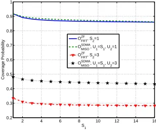
Fig. 2 shows that for U2 = S2 = 1 both ZF-FRT and
SDMA perform similarly. Furthermore, by increasingS1,
equivalentlyU1, the coverage probability in both systems is
slightly reduced. Nevertheless, for the setting, whereU2=
S2= 3, the coverage probability is reduced in both systems
while SDMA system over-performs ZF-FRT system. Multi-stream ZF-FRT system and multi-user SDMA system are fundamentally different as in the former all the transmitted streams to a user are required to be successfully received to consider that user in the coverage. Therefore, by fixing the density of the BSs the likelihood of successful reception of all streams might be generally lower. Nevertheless, in the multi-user SDMA each UE is only responsible for detecting its own single stream data. Of course the likelihood of successful reception for each individual stream might also reduce by increasing the number of UEs due to reduction of DoF and ICI increase however, the reduction is less than that of the ZF-FRT scheme. In terms of the complexity, multi-user SDMA for each UE requires perfect channel direction information to be able to construct the precoding matrix, whereas the ZF-FRT scheme does not require any feedback.
E. Orthogonal Space-Time Block Codes (OSTBCs) Systems
Recognizing the statistical resemblances of the SIR expres-sions among ZFBF and OSTBCs systems (see, e.g., [20]), the
2 4 6 8 10 12 14 16
0.2 0.3 0.4 0.5 0.6 0.7 0.8 0.9 1
S1
Coverage Probability
OZF FRT, S2=1 OSDMA
MISO, U1=S1, U2=1 OZFFRT, S2=3
[image:7.595.52.296.63.184.2]OSDMA MISO, U1=S1, U2=3
Fig. 2. Coverage probability of ZFBF and MISO-SDMA systems vs. S1, where λ1 = 10−4, λ2 = 5×10⁻³, α = 4,Nr = Nt
1 = N2t = 16, P1= 50W,P1= 10W,β1= 10dB,β2= 5.
analysis of this paper can readily be extended to the case of OSTBC systems. To do so, we need to assume that fading matrices, the positions of BSs and UEs, and their associations remain unchanged during the the space-time block codes. Ana-lyzing schemes, such as maximum ration combining (MRC) at the receiver while the transmitters do not have CSIT, are more complex due to the inter-stream interference at the receiver side.
VI. NUMERICAL ANALYSIS ANDSIMULATIONRESULTS
We now provide numerical and simulation results.K= 2is assumed for easier presentation of the results. We first focus on providing numerical analysis of coverage performance of FRT and ART schemes, aiming to shed light how multiplexing gains affect the strength of intending signals and interference. We then provide technical interpretations of the observed trends.
The second part of this section provides various simula-tion results to corroborate our analysis and investigate the impacts of densification and MIMO communications on the coverage performance. We also investigate the cases in which densification and MIMO communications are beneficial to the network’s coverage performance.
A. Numerical Analysis
To capture the impact of multiplexing gains on the coverage probability, we simply assumeβi=βandλi =λandPi=P.
1) The FRT Scheme: We start with the FRT scheme.
Proposition 1 provides an upper-bound of the coverage prob-ability. Here we consider the coverage probability for tieriin (6). Examination of (6) reveals two impacts of multiplexing gains: (i) the DoF of intending and interfering signals and (ii) the transmission power per stream on both attending and interfering signals. To distinguish them, we first exclude the impact of multiplexing gains on the transmission power per stream (it is equivalent to saying that the transmission power at BSs of tier j proportionally increases with Sj)).
We then define f1(S1) =∆ S1αˇ 1
Ã
Nr−S
1 P
r1=0
Γ(αˇ
S1+r1)
Γ(αˇ
S1)Γ(1+r1) !S1
and
f2(S1, S2) =∆
µ
Γ(αˇ
S1+S2)
Γ(S2) ¶S1
+
µ
Γ(αˇ
S1+S1)
Γ(S1) ¶S1
. It is easy to
observe that functions, f1(S1) and f2(S1, S2) represent the
For Peer Review
effect of multiplexing gains, S1, and S2, in the
numera-tor and the denominanumera-tor of (6) while the impact of power per stream is excluded. Moreover, we introduce functions
f∗
1(S1)andf2∗(S1, S2), respectively, as f1∗(S1)=∆S1−αˇf1(S1)
and f∗
2(S1, S2) =∆ S2−αˇ
µ
Γ(αˇ
S1+S2)
Γ(S2) ¶S1
+S−αˇ
1
µ
Γ(αˇ
S1+S1)
Γ(S1) ¶S1
so that the impacts of multiplexing gains on the transmit powers at the BSs are also captured. As it is seen from (6), OZFFRT,1 ∝ f
∗
1(S1)
f∗
2(S1,S2). Functions f1(S1) and f ∗
1(S1) can
be interpreted as tangible intended-DoF per communication
link, and effective intended-power per communication link,
respectively. Similarly, to capture the impact of multiplexing gains on the coverage performance per stream in (7), we define
g1(S1)∆=
Nr−S
1 P
r1=0
Γ( ˇα+r1)
Γ( ˇα)Γ(1+r1)andg2(S1, S2)
∆
= Γ( ˇα+S2)
Γ(S2) +
Γ( ˇα+S1)
Γ(S1) ,
while the effect of multiplexing gains on the power per stream is excluded. To incorporate this, we further define g∗
1(S1) ∆ =
S−αˇ
1 g1(S1) andg∗2(S1, S2)=∆S−2αˇ Γ( ˇα+S2)
Γ(S2) +S
−αˇ 1
Γ( ˇα+S1)
Γ(S1) . It is
then easy to verify from (7) thatOZFFRT,1,li∝ g
∗
1(S1)
g∗
2(S1,S2).
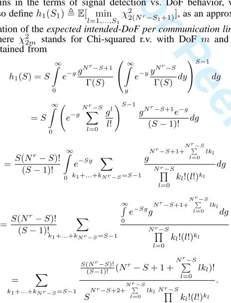
On the other hand, to inspect the impact of multiplexing gains in the terms of signal detection vs. DoF behavior, we also defineh1(S1),E[ min
l=1,...,S1 χ2
2(Nr−S1+1)], as an approxi-mation of the expected intended-DoF per communication link, where χ22m stands for Chi-squared r.v. with DoF m and is obtained from
h1(S) =S
∞ Z
0
e−gg
Nr−S+1
Γ(S)
∞ Z
g
e−yy
Nr−S
Γ(S) dy
S−1
dg
=S
∞ Z
0
à e−g
NXr−S
l=0
gl
l!
!S−1
gNr−S+1
e−g
(S−1)! dg
= S(N
r−S)!
(S−1)!
∞ Z
0
e−Sg X
k1+...+kN r−S=S−1
gN
r−S+1+N rP−S l=0
lkl
NrQ−S
l=0
kl!(l!)kl
dg
=S(N
r−S)!
(S−1)!
X
k1+...+kN r−S=S−1
∞ R
0
e−SggNr−S+1+
N rP−S
l=0 lkl
dg
NrQ−S
l=0
kl!(l!)kl
= X
k1+...+kN r−S=S−1
S(Nr−S)! (S−1)! (N
r−S+ 1 +N
r−S
P
l=0
lkl)!
SN
r−S+2+N rP−S l=0
lklNrQ−S
l=0
kl!(l!)kl
.
This way, k1(S1),Nr−S1+ 1is actually the expected
intended-DoF per stream. Contrastingh1(S1)(k1(S1)) against
functions f1(S1)and f2(S1, S2)(g1(S1)and g2(S1, S2))
re-veals how much of the expected DoF is actually helpful in im-proving the ability of the receivers in detecting signals. Finally, we defineh∗
1(S1) =S1−αˇh1(S1)andg∗1(S1) =S1−αˇg1(S1)as
the overall representations of the multiplexing gains on the expected DoF per link and per stream, respectively.
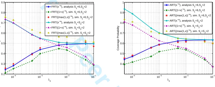
Fig. 3 plots f1(S1) and g1(S1) vs. S1. Both f1(S1) and
g1(S1) are shown to be monotonically decreasing functions
of S1, and hence increasing the multiplexing gainS1 results
in a lower coverage probability from both link and stream per-spectives. Further,f1(S1)is shown to be smaller thang1(S1),
so per-link coverage probability is much smaller than the that of per-stream. Therefore, per-link and per-stream coverage probabilities react differently to changes in the multiplexing gain.
[image:8.595.59.291.297.602.2]We further study the impact of transmission power in Fig. 3, where f∗
1(S1) and g∗1(S1) are presented for various
multiplexing gains. Figs. 3 shows similar patterns. The main difference is that by increasingS1,f1∗(S1)andg1∗(S1)decline
more quickly thanf1(S1)andg1(S1). Moreover, we observe
that values of functions f1(S1) and g1(S1) are in general
much smaller than that of h1(S1) and k1(S1), respectively.
Consequently, the expected DoF can be considered as opti-mistic measures of the receiver’s capability in terms of signal detection.
Fig. 4 demonstratesf2(S1, S2) andg2(S1, S2). Both
func-tions are shown to exhibit the same pattern by varying S1
andS2, where generally f2(S1, S2)≤g2(S1, S2). Therefore,
by reducing the multiplexing gain,S1, the negative impact of
ICI on the performance of a communication link is reduced, compared to the performance of a given stream. We also observe that by increasing S2, both functions are increased.
By incorporating the impact of power, however, the observed behavior is dramatically changed as shown in Fig. 4, where
f∗
2(S1, S2) and g2∗(S1, S2) are given vs. S1. One can see
that (i) there are meaningful discrepancies between functions
f∗
2(S1, S2)andg2∗(S1, S2)not only from their corresponding
values but also from their behaviors with respect to S1; (ii)
whilef2(S1, S2)andg2(S1, S2)are monotonically increasing
functions ofS1(left plot),f2∗(S1, S2)demonstrated decreasing
and mildly increasing patterns depending on S1. Function
g∗
2(S1, S2)is also slightly increased by increasingS1.
Combining the findings of Figs. 3 and 4, we conclude that increasing the multiplexing gains reduces the coverage proba-bility. Furthermore, the main reason for higher multiplex gains resulting in a smaller coverage probability is due to the im-pairing impact of multiplexing gains on the effective intended-power per communication link, noticing the flat response of functionf∗
2(S1, S2)toS1 in Fig. 4 as well as a sharp drop of
functionf∗
1(S1)toS1in Fig. 3. To confirm this conclusion, we
setS1 =S2=S, and illustrate per-link coverage probability
(6) and per-stream coverage probability (7) vs. parameter S
in Fig. 5. Both interpretations of the coverage probabilities are shown to be monotonically decreasing functions of S. According to Fig. 5, increasing the multiplexing gain from
S= 1toS = 2reduces the coverage probability per link by more than30%, with an almost15%reduction in the coverage probability per stream.
ForNr=Si,∀i,
OZF
FRT≤ ˜ π
C(α)βαˇ 1
Sαˇ
µ
Γ(S)
Γ(ˇα/S+S)
¶S
. (16)
Using Kershaws inequality (see, e.g., [37]), we write
Γ(αˇ
S+S)
Γ(S) >
µ S+αˇ
S −1 +
1−α/Sˇ
2
¶αˇ
S
=
µ S+
ˇ
α S−1
2
¶α/Sˇ
.
(17)
For Peer Review
2 4 6 8 10 12 14 16 18 20 0
5 10 15 20 25
S 1
Values of Functions
f 1(S1) f* 1(S1) h1(S1)
h* 1(S1) g
1(S1) g*
1(S1) k
1(S1) k*
[image:9.595.66.543.59.183.2]1(S1)
Fig. 3. f1(S1),g1(S1),h1(S1), andk1(S1)vs. S1forK= 2,Nr= 20, andα= 3.5.
2 4 6 8 10 12 14 16 18 20 1
2 3 4 5 6 7 8
S 1
Values of Functtions
f 2(S1,S2),S2=1 f
2(S1,S2),S2=4 g
2(S1,S2),S2=1 g
2(S1,S2),S2=4 f*
2(S1,S2),S2=1 f*
2(S1,S2),S2=4 g*
2(S1,S2),S2=1 g*
2(S1,S2),S2=4
Fig. 4. f∗
1(S1),g∗
1(S1),h∗
1(S1), andk∗
1(S1)vs. S1forK= 2,Nr= 20, andα= 3.5.
2 4 6 8 10 12 14 16 18 20 0
0.1 0.2 0.3 0.4 0.5 0.6 0.7
S
Coverage Probability
OZFFRT,α=4.5 OZFART, α=4.5 OZFFRT,α=3.5 OZFZRT,α=3.5
Fig. 5. Coverage probability of the ART and FRT schemes vs.S, whereλi=λ,Pi=P, andβi= β,∀i.
Substituting (17) into (16) yields OZF
FRT ≤
π
˜
C(α)βαˇ
1
Sαˇ(1−S−1) ³
1 +α/Sˇ2S−1
´−αˇ
which is a decreasing function of S. Thus, increasing the multiplexing gain S
reduces the coverage probability.
Note that the above numerical and analytical results are based on the upper-bound given in Proposition 1. The sim-ulation results presented in the next subsection confirm the accuracy of Proposition 1, and thus the conclusions drawn here remain valid.
2) The ART Scheme: We consider ART scheme for which the corresponding coverage probability is approximated in Proposition 2. According to Proposition 2, its coverage probability is proportionally related to the coverage prob-ability of FRT. Thus, the above numerical analysis would stay valid in the case of ART. Note that comparing with the bound for the coverage probability of the FRT scheme given in (5), understanding the impact of the multiplexing gains even in the simplified scenario of this subsection is not straightforward. Therefore, we rely on a numerical analysis by comparing the approximation in (11) with the bound given in Proposition 1.
In Fig. 5, (5) and (11) are plotted for a system withK= 2, and S1 = S2 = S. The ART scheme is shown to perform
significantly better than FRT. For instance, when S= 4, and
α= 4.5, adopting the ART scheme makes a more than 45% coverage performance improvement over the system with FRT. The modest cost of this improvement is the extra signaling overhead caused by the UEs feeding back to the BSs the achievable data rates for each stream. Fig. 5 also suggests that compared to the FRT scheme, in the ART scheme the coverage performance diminishes faster by increasing the multiplexing gain. For instance, by increasing the multiplexing gain from
S = 1 to S = 2, the coverage performance of FRT (ART) is reduced by 30% (10%). Fig. 5 further indicates that the coverage performance of ART is more sensitive to the variation of the path-loss exponent than that of FRT. Therefore, the FRT scheme demonstrates a level of robustness against changes (e.g., from outdoor to indoor) in the wireless environment.
B. Simulation Results
In our simulation we set K = 2 and randomly locate BSs of each tier in a disk of radius 10000 units according to the corresponding deploying density. All BSs are always
10−1 100 101
100
β2
Coverage Probability
FRT, sim. S
1=S2=2
ART, sim. S1=S2=2, FRT, analysis S1=S2=2 ART, analysis S1=S2=2 FRT, sim. S
1=6,S2=2
ART, sim. S1=6,S2=2 FRT, analysis S1=6, S2=2 ART, analysis S1=6, S2=2
Fig. 6. Coverage probability of the FRT and ART scheme v.s.β2, where
λ1 = 10−4,λ2= 5×10⁻⁴,α= 4,Nr = 10,P
1 = 50W,P1= 10W,
β1= 5.
active and the simulation is run for40000snapshots. In each snapshot, we randomly generate MIMO channels based on the corresponding multiplexing gains at the BSs.
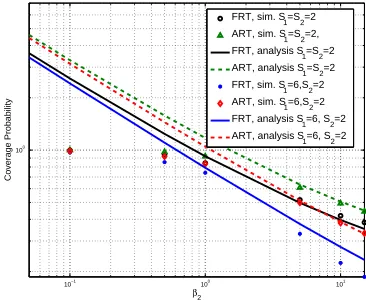
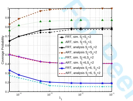
1) Accuracy of the Bounds: Fig. 6 plots the coverage
probabilities under FRT and ART schemes vs.β2. As shown
for β2 ≥ 1, which is the case of our model, the analytical
bounds closely follow the simulation results. This finding is important especially for the case of ART as the proposed bound in (11) is heuristic. For the case of β2 <1, however,
the analysis is not representative. Therefore, Fig. 6 confirms the results reported in [16], [26]. We further observe that by increasingβ2, the coverage probability is reduced in all graphs
and ART outperforms FRT. In both schemes, by increasing the multiplexing gain, S1, the corresponding coverage
probabili-ties are shown to be reduced.
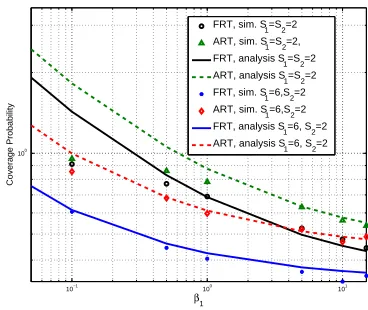
Fig. 7 compares the analysis and simulation results vs. β1,
showing the same patterns observed in Fig. 6. However, comparison of Figs. 6 and 7 shows that increasingβ1 makes
less impact on reduction of the coverage probability in both schemes.
From the comparison of Figs. 7 and 6, we also find that increasing β2 widens the gap between FRT and ART while
the growth ofβ1 narrows the gap. The observed discrepancies
are due to the differences between the transmission power and densities of the BSs in different tiers.
We also evaluate the accuracy of our analysis against the
[image:9.595.343.526.228.379.2]For Peer Review
10−1
100
101 100
β1
Coverage Probability
FRT, sim. S1=S2=2 ART, sim. S1=S2=2, FRT, analysis S1=S2=2 ART, analysis S
1=S2=2
FRT, sim. S1=6,S2=2 ART, sim. S1=6,S2=2 FRT, analysis S1=6, S2=2 ART, analysis S
[image:10.595.344.527.56.219.2]1=6, S2=2
Fig. 7. Coverage probability of FRT and ART scheme v.s.β1 whereλ1= 10−4,λ2= 5×10⁻⁴,α= 4,Nr= 10,P1= 50W,P1= 10W,β2= 5.
density of BSs deployment in Figs. 8 and 9. In the former (the latter), we fix λ1 = 10−4 (λ2 = 10−4) and change λ2 (λ1).
Both figures confirm that the proposed approximations for both FRT and ART closely follow the corresponding coverage probability. This also confirms our conclusion on the impact of the multiplexing gains on the coverage performance of FRT and ART in the previous sections.
2) Impact of Multiplexing Gains and Densifications: Figs. 8
and 9 also highlight the following important trends. (i) ART provides better coverage performance than FRT by almost 20– 25%, which is smaller than our previously expected value in Section IV-B. This is because in Section IV-B, transmission powers, deploying densities, and SIR thresholds are assumed to be the same in both tiers. One may conclude that the advan-tage of ART over FRT is fully exploitable in a homogenous network deployment, i.e., Pi = P, Si = S, λi = λ, and
βi =β ∀i. (ii) Multiplexing gains S1 and S2 make different
impacts on the coverage performance: (ii-1) According to Fig. 8, while the density of high-power BSs in tier 1, λ1,
is fixed, if S1 = S2, increasing λ2 lowers the coverage
probability. On the contrary, Fig. 9 indicates that when the density of low-power BSs in tier 2, λ2, is fixed by increasing
λ1, a higher coverage performance results forS1=S2. In fact,
for cases with the same multiplexing gain across the tiers, the coverage probability could decrease/increase depending upon the densified tier. Therefore, in such cases it is more efficient to densify the tier with the higher transmission power.
(ii-2) Fig. 8 shows that for fixed λ1, increasingλ2 is beneficial
and results in a higher coverage performance, where S1= 6,
and S2 = 2. Fig. 9, on the other hand, illustrates that for
S1 = 6 and S2 = 2 and when λ2 is fixed, increasing λ1
lowers the coverage probability. Consequently, in cases with different multiplexing gains, the results suggest that it is better to densify the tier with low-power and/or low multiplexing gain. (ii-3) For high values of λ2, Fig. 8 also shows that
both cases of S1 = 6, S2 = 2 and S1 = S2 = 2 perform
the same. For high values of λ1, Fig. 9, however, shows a
large gap between the coverage probability of systemS1= 6,
S2= 2and that of systemS1=S2= 2. In other words, for a
network with ultra-dense low-power tier, the multiplexing gain
10−4 10−3 10−2 10−1 0.2
0.3 0.4 0.5 0.6 0.7 0.8 0.9 1
λ2
Coverage Probability
[image:10.595.79.263.62.217.2]FRT, sim. S1=S2=2 ART, sim. S1=S2=2, FRT, analysis S1=S2=2 ART, analysis S1=S2=2 FRT, sim. S1=6,S2=2 ART, sim. S1=6,S2=2 FRT, analysis S1=6, S2=2 ART, analysis S1=6, S2=2
Fig. 8. Coverage probability of the FRT and ART schemes vs.λ2, where
λ1 = 10−4,α = 4,Nr = 10,P1 = 50W,P1 = 10W, β1 = 2, and β2= 5.
of high-power tier can be increased without compromising the coverage performance.
In summary, increasing the density of low power BSs (tier 2) should be interpreted as a green light for increasing the multiplexing gain of tier 1 without hurting the coverage performance. Moreover, densification in tier 1 results in a higher performance provided that similar multiplexing gains are set across all tiers.
(iii) The results in Figs. 8 and 9 also indicate that increasing the density of low power BSs of tier 2 makes greater impact on the coverage probability than it does in tier 1. For instance, a 10-fold densification of tier 2 (tier 1) changes the coverage performance by more than25% (10%). This is a very impor-tant practical insight because installing more low-power BSs
is cheaper than increasing the density of high-power BSs of tier 1.
(iv)The above results also confirm that for large values ofλ1
andλ2, the coverage probability is stable and does not react
to densification. This is also referred to as scale invariancy, see, [16]. This indicates that we could increase the capacity by installing more BSs without hurting the coverage. As a result, without sacrificing the coverage performance, we can increase the density of BSs in tier 2 to simultaneously increase the multiplexing gain of tier 1.
3) Impact of Number of Receive Antennas: In Figs. 10 and
11, we study the impact of the number of receive antennas
Nr on the coverage performance. We first review the results
of Fig. 10, where a sparse tier 1 with the density of BSs,
λ1 = 5×10⁻⁵, is considered. Two scenarios are considered
with respective to the density of BSs in tier 2: (1) dense, the results of which are shown in the left plot, and (2) sparse, the results of which are given in the right panel. In both cases, we investigate three cases: (1) S1 = S2 = 1, (2) S1 = Nr,
S2 = 1, and (3) S1 = S2 = Nr. In both dense and sparse
scenarios, the case ofS1=S2=Nrperforms very poorly and
increasing the number of antennas worsens performance. In this case, ART slightly outperforms FRT. Moreover, for small values ofNr, the sparse scenario yields a better performance than that of the dense scenario. For large values of Nr,