Discriminant Analysis via Joint Euler Transform and ℓ2, 1 Norm

(1)

Discriminant Analysis via Joint Euler Transform

and

`

₂

_,

₁

-norm

Shuangli Liao, Quanxue Gao, Zhaohua Yang, Fang Chen, Feiping Nie, and Jungong Han

Abstract—Linear Discriminant analysis (LDA) has been widely used for face recognition. However, when identifying faces in the wild, the existence of outliers that deviate significantly from the rest of data can arbitrarily skew the desired solution. This usually deteriorates LDA’s performance dramatically, thus preventing it from mass deployment in real-world applications. To handle this problem, we propose an effective distance metric learning method based LDA, namely Euler LDA-L21 (e-LDA-L21). e-LDA-L21 is carried out in two stages, in which each image is mapped into a complex space by Euler transform in the first stage and the`2,1 -norm is adopted as the distance metric in the second stage. This not only reveals nonlinear features but also exploits the geometric structure of data. To solve e-LDA-L21 efficiently, we propose an iterative algorithm, which is a closed-form solution at each iteration with convergence guaranteed. Finally, we extend e-LDA-L21 to Euler 2DLDA-e-LDA-L21 (e-2DLDA-e-LDA-L21) which further exploits the spatial information embedded in image pixels. Experimental results on several face databases demonstrate its superiority over the state-of-the-art algorithms.

Index Terms—Linear Discriminant Analysis, Two-dimensional Linear Discriminant analysis, Dimensionality reduction, Euler transform, `2,1-norm.

I. INTRODUCTION

F

INDING an effective representation for image has been a fundamental problem in the fields of pattern recognition and machine learning. During the last few decades, many approaches have been developed for this task, among which principal component analysis (PCA) [1] and linear discrim-inant analysis (LDA) [2] turn out to be two representatives. PCA is a unsupervised method used for extracting the most representative features, while LDA is a supervised one capable of extracting the most discriminative features. Not surprisingly, LDA generally performs better when conducting data classi-fication task.

In the domain of image analysis, it is essential to reshape the original two-dimensional image into a high-dimensional

Manuscript received Jan, 2016; revised ********; accepted ********. This work is supported by National Natural Science Foundation of China under Grant 61773302, the 111 Project of China (B08038), and Shenzhen Fundamental Research fund under Grant JCYJ20160530141902978.

Corresponding author: Q. Gao (e-mail: xd ste [email protected]) and Z. Yang ([email protected]).

The authors wish it to be known that, in their opinion, the first and third authors should be regarded as joint First Authors

S. Liao, Q. Gao and F. Cheng are with State Key Laboratory of Integrated Services Networks, Xidian University, 710071, Xi’an CHina

Z. Yang is with the School of Instrumentation Science and Opto-electronics Engineering, Beihang University, Beijing, China

F. Nie is with the Center for OPTical IMagery Analysis and Learning, Northwestern Polytechnical University, 710069, Xi’an China.

J. Han is School of Computing and Communications, Lancaster University, United Kingdom.

vector prior to applying the aforementioned methods. This may impair the spatial structure information embedded in the pixels of image. To tackle this problem, many image matrix-based dimensionality reduction methods have been developed, most of which follow the idea of directly estimating the scatter matrices from image matrices and then solving the projection matrix by optimizing the criterion function. Such matrix based methods include two-dimensional PCA (2DPCA) [3], multi-linear PCA [4], two-dimensional LDA (2DLDA) [5], tensor LDA [6], and direction tensor independent component analysis [7]. Despite the impressive results obtained in many cases, these approaches struggle with the outliers existed in the real-life applications. The reason behind is that all of the above approaches characterize the geometric structure of data by squared`2-norm, which is not robust in the sense that outlying

measurements would arbitrarily skew the acquired solution from the desired solution [8] [9].

Most existing works have demonstrated that distance metric learning based methods can effectively improve the robust-ness of algorithms against outliers [10]–[18]. Team Bischof proposed KISSME metric learning [10], which is based on a statistical inference perspective. Martinelet al.[11] proposed a Kernelized Saliency-based method for multiple metic learing.

Li et al. [12] integrated the distance metric to the SVM

decision fuction. Alternatively, Liao et al. [13] incorporated the dimension reduction and metric learning, and further used the PSD constraints [14] to enhance the robustness of the learned metric. To handle the small sample size (SSS) problem, Zhang et al. [15] proposed a method by matching samples in a discriminative null space of the training data. It is noted that there are some other methods based on temporal model [16] and video [17].

Compared to squared`2-norm, nuclear-norm [19] [26] and

`1-norm [20]–[26] are more robust to outliers for

dimension-ality reduction. Using nuclear-norm as the distance metric, Zhang et al. [26]. proposed nuclear-norm based 2DPCA (N-2DPCA) that seeks the projection matrix by minimizing the nuclear-norm based reconstruction error. Similarly, many sub-space learning methods employ`1-norm as the distance metric

in order to obtain more robust projection vectors. For example, L1-PCA [20] employed `1-norm to calculate the

reconstruc-tion error, which was minimized afterwards via a greedy algorithm. To further speed up the L1-PCA algorithm, Kwak [21] proposed to seek the projection vectors by maximizing the `1-norm variance. This method is called PCA-L1, which

(2)

non-greedy 2DPCA-L1 [24]. To encode the discriminant infor-mation better, some `1-norm based LDA methods have been

developed for image classification [27]–[30]. Two of the most popular methods are LDA-L1[28] and l1-norm based kernel LDA [29], where the former used l1-norm to calculate the within-class scatter matrix and between-class scatter matrix, while the latter employed l1-norm as the distance metric in kernel LDA. Liu et al. [31] and Wang et al. [32] proposed non-greedy algorithms to solve `1-norm based discriminant

analysis methods, which can optimize the criterion function. To well exploit discriminant spatial structure, Li et al. [33] proposed L1-2DLDA for image classification.

However,`1-norm subspace methods do not well

character-ize the geometric structure due to the fact that the solution of `1-norm subspace methods relates nothing to scatter

ma-trices that characterize the geometric structure of data [34]– [36]. Moreover, `1-norm based subspace techniques cannot

provide the subspace with join-feature spareseness [37]–[41]. To handle this problem, Ding et al. [35] developed `2,1

-norm and used it to estimate the reconstruction error of data. Based on it, a novel method R1-PCA, which seeks low-dimension space by minimizing`2,1-norm reconstruction error,

was proposed to improve the robustness of PCA. Nieet al.[38] showed that`2,1-norm helps select useful features from

high-dimensional data. Inspired by these works,`2,1-norm has been

widely used as the regularization term in the criterion function. For example, Wong et al. [40] proposed `2,1-norm based

tensor feature selection for image analysis. Gui et al. [37] used `2,1-norm as the regularized term in subspace learning

and proposed a joint feature extraction and selection method for data classification. Since all of them still used squared Euclidean distance to measure the similarity between data, the flexibility and robustness of the algorithms are adversely affected. Moreover, for image classification, most existing discriminant methods still measure the similarity in the pixel space, thus leading the methods to be sensitive to illumination and outliers. Finally, the aforementioned robust discriminant methods do not reveal non-linear features which can actually help improve the robustness of algorithms.

Motivated by the fact that kernel trick can capture the nonlinear features [42]–[44] and combine the superiority of `2,1-norm, in this paper, we develop a distance metric learning

based robust LDA, namely e-LDA-L21, for discriminative feature extraction. e-LDA-L21 first maps the original images into the complex space by Euler transform, which not only suppresses outliers but also reveals non-linear patterns em-bedded in data. Afterwards, it uses`2,1-norm to measure both

between-class scatter matrix and within-class scatter matrix in the complex space. Likewise, we further extend this concept to handle 2D data and propose an e-2DLDA-L21 algorithm. Experimental results reveal the effectiveness of our proposed method. In contrast to most existing robust subspace methods, we have the following contributions:

• By analyzing Euclidean distance,`1-norm, and`2,1-norm,

we have showed that`2,1-norm can help enlarge the role

of small between-class distance and weaken the effect of large between-class distance. Thus, we employ `2,1

-norm as the distance metric in LDA. This helps improve

the robustness of LDA against to outliers.

• Our method extracts nonlinear features with Euler

trans-form in LDA. Different from the commonly used kernel function, which maps data into a higher-dimensional hidden space, Euler transform maps data into an explicitly space which has the same dimensionality as that in the original data space. As a result, our method can be easily implemented in real applications. Moreover, we have showed that cosine distance metric not only helps obtain a large margin but also improves the separability between different class images. Thus, our method well encodes nonlinear discriminant features and simultaneously gets a large margin which is important for classification.

• Our method integrates both kernel trick and distance metric learning into the criterion function. It helps fur-ther improve the robustness of algorithm. Moreover, the proposed iterative algorithm has a good convergence. The remainder of this paper is organized as follows. Section 2 reviews the related work.`2,1-norm-based LDA with Euler

representation, namelye-LDA-L21, is proposed in Section 3. We extende-LDA-L21 toe-2DLDA-L21 in Section 4. Section 5 reports experimental results. Finally, the conclusions are drawn in Section 6.

II. LINEARDISCRIMINANTANALYSIS

Assume that we haveN training imagesXj ∈Rm×n(j=

1,2, ..., N), where m andn denote the number of rows and columns of an image, respectively. The given data have c classes and the ith class has ni samples. X¯i andX¯ denote

the class mean image of the ith class and the mean image of all image samples, respectively. Denote xj, ¯xi and x¯

∈RM×1₍_M ₌_m_×_n₎ _{by the vector forms of matrices} _X

j, ¯

Xi andX¯, respectively, i.e., xj=vect(Xj),¯xi =vect(X¯i),

and¯x=vect(X¯).

A. LDA and 2DLDA

LDA aims to seek the projection matrix W= [w1,w2,· ·

·,wd]∈RM×d which minimizes the within-class scatter and

simultaneously maximizes the between-class scatter in the low -dimensional space. The objective function of LDA is [2]

Wopt= arg max

wkTwk=1

tr(WTSbW)

tr(WT_S

wW)

(1)

where wk(k = 1,2,· · ·, d) is the kth column of the matrix

W,tr(·)is the trace operator of a matrix, between-class scatter matrixSband within-class scatter matrixSware defined as

Sb=

c

X

i=1

ni(¯xi−x¯)(¯xi−¯x) T

(2)

Sw=

c

X

i=1

X

j∈ci

(xj−¯xi)(xj−¯xi) T

(3)

whereci denotes the ith class data set.

(3)

(1). Hence, such problems are often transformed into the simpler yet inexact ratio trace problem, which is equivalent to the determinant ratio problem [45]. For the model (1), the corresponding ratio trace (determinant ratio) form is

Wopt= arg max

W

tr WTSwW

−1

WTSbW

(4)

The optimal projection matrix Wopt of the objective

func-tion (4) consists of the eigenvectors{wk|k= 1,2,· · ·, d} of

the Eigen-equation (Sw) −1

Sbwk = λkwk corresponding to

the firstdlargest eigenvalues {λk|k= 1,2,· · · , d}.

Each image needs to be transformed into a 1D vector in LDA-based methods. Thus, they can no longer exploit the spatial information embedded in pixels. To handle this problem, 2DLDA is one of the most representative methods. In order to be consistent with the existing improved methods, such as L1-2DLDA [33], the model of 2DLDA only considers the left projection here. The model is

Qopt= arg max

qkTqk=1

tr QT_G

bQ

tr(QT_G

wQ)

(5)

where Q= [q1,q2, ...,qd]∈Rm×d andqk(k= 1,2,· · · , d)

is the k-th column of the matrix Q, between-class scatter matrix Gb and within-class scatter matrixGw are defined as

Gb =

c

X

i=1

ni X¯i−X¯

_¯

Xi−X¯

T

(6)

Gw=

c

X

i=1

X

j∈ci

Xj−X¯i

T

(7)

By simple algebra, the nominators and denominators of the objective functions (1) and (5) can be respectively rewritten as

tr(WTSbW) =

c

X

i=1

ni

WT(¯xi−¯x)

2

2 (8)

tr(WTSwW) =

c

X

i=1

X

j∈ci

WT(xj−¯xi)

2

2 (9)

tr QT_G

bQ = c P i=1 ni n P k=1

QT X¯i(:, k)−X¯(:, k)

2 2

(10)

tr QT_G

wQ=

c

P

i=1

P

j∈ci

n

P

k=1

QT Xj(:, k)−X¯i(:, k) 2 2

(11) whereX¯i(:, k)andXj(:, k)denote thekth column of matrices

¯

Xi andXj, respectively.

As can be seen in Eqs. (8), (9), (10) and (11), the large distance will remarkably dominate the solution of the models (1) and (5). Thus, the optimal solution of the objective function (1) and (5) is susceptible to the presence of outliers which deviate significantly from the rest of data. Moreover, squared `2-norm can suppress the role of small between-class scatter

in the criterion function. Thus, traditional LDA technique is unlikely to obtain a large margin, which is important for classification, in the low-dimensional space.

B. LDA-L1 and L1-2DLDA

To improve the robustness of discriminant analysis tech-nique, many enhanced discriminant methods have been de-veloped, among which LDA-L1 and L1-2DLDA [33] are two of the most representative methods. The objective function of LDA-L1 is

Wopt= arg max

wkTwk=1 c

P

i=1

ni

WT(xi−x)

1 c P i=1 P

j∈ci

kWT₍_x

j−xi)k₁

(12)

L1-2DLDA aims to seek projection matrixQby the model (13).

Qopt= arg max

qkTqk=1 c

P

i=1

ni

QT Xi−X

_L₁ c P i=1 P

j∈ci

QT Xj−Xi

_L₁

(13)

wherek•k_L₁ denotes the `1-norm of a matrix which can be

defined askXk_L₁=P

k

kX(:, k)k₁,X( :, k)is thekth column

of matrixX.

Although the linear discriminant analysis technique based on `1-norm is robust to outliers, compared with traditional

LDA, the solutions of both the models (13) and (12) are irrelevant to the scatter matrices that characterize the geometric structure. Thus, neither LDA-L1 nor L1-2DLDA can well reveal the geometric structure that is crucial for classification. Moreover, it is difficult to solve`1-norm optimization problem.

Consequently, it is unclear whether`1-norm can help improve

the role of small between-class scatter in the models (13) and (12).

III. EULERLDA-L21

A. Motivation

As can be seen from the above analysis,squared Euclidean

distanceactually makes the outlying measurements dominate

the solution of the objective function (1). This leads the ob-jective function (1) to be more prone to the outliers. To handle this problem, the distance metric in the model (1) should not only suppress the outliers but also enlarge the role of small between-class scatters. Combining the aforementioned analysis and the recent works [42] [43], we present an efficient and robust LDA for dimensionality reduction. It aims to seek a robust projection matrixWsuch that the projected data can well reveal not only discriminant geometric structure of data but also non-linear features.

Prior to formulating the proposed method, we first introduce the definition of`2,1-norm and cosine distance metric that can

be viewed as a kernel function [42] [43], and then analyze their advantages to outliers and discriminant geometric structure.

Definition 1 [35]. Given an arbitrary matrixA= [A(i, j)]∈

Rm×n_{, the}_`

2,1-norm of matrix Ais defined as

kAk_L

2,1 =

n

X

j=1

r Xm

i=1A

2₍_{i, j}_{) =}

n

X

j=1

kA(:, j)k₂ (14)

(4)

-2 0 2 4 6 8 10 12 -6

-4 -2 0 2 4 6

class1 class2

class3 outlier

W LDA- L21 W

LDA- L1 W

LDA - squared L2 Woutlier

LDA- L21 Woutlier

LDA- L1 Woutlier

LDA- squared L2

(a)

-6 -4 -2 0 2 4 6 8

W_LDA-L21 -1

0 1

-6 -4 -2 0 2 4 6 8

W_LDA-L1 -1

0 1

-2 0 2 4 6 8 10 12

W_{LDA-squared L2} -1

0 1

(b)

-4 -2 0 2 4 6 8 WoutlierLDA-L21

-1 0 1

-6 -4 -2 0 2 4 6 8 WoutlierLDA-L1

-1 0 1

-4 -2 0 2 4 6 8 Woutlier

LDA-squared L2

-1 0 1

(c)

Figure1. (a) Directions of LDA, LDA-L21 and LDA-L1; (b) projected data of LDA, LDA-L21 and LDA-L1; (c) projected data of LDA, LDA-L21 and LDA-L1 with outliers.

essential difference with squared`2-norm. Thus, if`2,1-norm

is employed as the distance metric in the criterion function, it can well reveal the geometric structure of data. Moreover, compared with squared `2-norm, `2,1-norm can further help

enlarge the role of small between-class distance and weaken the effect of large between-class distance in the criterion function. This results in not only the enhanced robustness to outliers but also a large margin in the low-dimensional space, thus improving the performance of algorithm. For example, we randomly produce three classes data points, which are marked with different shapes and each class has 20 data points. The

three data classes follow Gaussian distribution with covariance matrices being [0.3 0; 0 0.3] and means being [0.5 -0.5] and [0 2], and [10 -1], respectively. Moreover, we also add two outliers whose color is green. Two outliers belong to the second class. Taking these data points as training samples, we show the directions of LDA, LDA-L21, and LDA-L1, and the corresponding low-dimensional representation in Figure 1.

WLDA,WLDA−L21andWLDA−L1 denote the directions of

LDA, LDA-L21 and LDA-L1 respectively when training data do not include outliers.Woutlier_LDA ,W_LDAoutlier₋_L₂₁andWoutlier_LDA₋_L₁

denote the directions of the aforementioned methods when training data have outliers. As can be seen in Figure 1, when training data are clean, LDA with`2,1-norm as distance metric

obtains a large margin between class 1 and class 2 in the low-dimensional space and well separates all classes in the low-dimensional space, whereas traditional LDA and LDA-L1 do not. When training data include outliers, both our model and LDA can correctly classify all data, while LDA-L1 does not. Moreover, our model achieves a larger margin than LDA. This observation motivates us to employ`2,1-norm as distance

metric in LDA criterion function.

Figure 2. Examples motivating the use of the cosine-based dissimilarity measure. Images from left to right are the original image, a second image of the same subject, an occluded version of the original image and an image of another subject.

Figure 3. Examples motivating the use of the cosine-based dissimilarity measure. Images from left to right are the original image, a second image of the same subject, an illumination change version of the original image and an image of another subject.

Definition 2 [42] [43]. Given two arbitrary vectorsxp and xq ∈RM×1, the cosine distance metric between them is

d(xp,xq) = M

X

k=1

{1−cos (απ(xp(k)−xq(k)))} (15)

whereαis an alpha mask [42], which is also known as alpha matte or alpha channel and associates variable transparency with an image.xp(k)andxq(k)are thek-th element of xp

(5)

TABLE I

COMPARISON OF NORMALIZED DISSIMILARITY MEASURES BETWEEN

IMAGES INFIGURE2.

Dissimilarity metric A-B A-C A-D

Euclidean distance 6.5437 11.5016 8.5694

`1-norm distance 158.2643 326.4584 275.6062

Cosine-based distance 352.1622 622.0739 851.188

TABLE II

COMPARISON OF NORMALIZED DISSIMILARITY MEASURES BETWEEN

IMAGES INFIGURE3.

Dissimilarity metric A-B A-C A-D

Euclidean distance 1.2629 16.4548 13.1405

`1-norm distance 29.6755 450.4374 359.8113

Cosine-based distance 28.0423 1159.577 1240.738

By simple algebra, Eq. (15) becomes

d(xp,xq)= M

P

k=1

{1−cos (απ(xp(k)−xq(k)))}

=1 2 M X k=1 n

(cosαπxp(k)−cosαπxq(k))2

+(sinαπxp(k)−sinαπxq(k))

2o = 1 √

2(e

iαπxp₋_eiαπxq₎

2

2 =kzp−zqk

2 2

(16)

where

zq =

1 √ 2   

eiαπxq(1)

.. . eiαπxq(M)

  = 1 √ 2e

iαπxq ₍₁₇₎

is called Euler representation of xq.

Eq. (16) illustrates that cosine distance metric between two images in the pixel space is equivalent to the squared `2-norm between the corresponding two images with Euler

representation.

Let us consider two motivating examples in which different dissimilarity measures are applied to the images that are shown in Figure 2 and Figure 3. Table I and Table II list the Euclidean distance,`1-norm distance and cosine distance metric between

images in Figure 2 and Figure 3, respectively. As can be seen in Figure 2, Figure 3, Table I and Table II, Euclidean distance and`1-norm distance associate a smaller distance between the

original image and an image from a different subject, while the distance between image A and image C, which belong to the same person with occlusion or different illumination, is large. In contrast, the use of the cosine-based measure results in a large distance between images that are from different persons. Combining the aforementioned analysis, we have the fol-lowing interesting observations:

• First, the cosine distance metric enlarges the distance between all images, so cosine distance metric can be beneficial to the data classification.

• Second, the distance between the same class images is enlarged a smaller multiple than the distance between the different class images by the cosine distance metric. This clearly shows that cosine distance metric not only helps obtain a large margin but also improves the separability

between different class images, compared with Euclidean distance and`1-norm.

B. Objective function

To improve the robustness of discriminant analysis tech-nique, we present our model with the aforementioned analysis, which employs`2,1-norm as the distance metric to measure the

similarity between data in the Euler space. Specifically, we first map each imagexq onto the Euler space by Eq. (17) and then

use`2,1-norm to reveal within-class and between-class scatter

matrices in the Euler space. Our model is as follows.

Wopt= arg max

wkHwk=1 c

P

i=1

ni

WH(¯zi−¯z)

₂ c P i=1 P

j∈ci

kWH₍_z

j−¯zi)k2

(18)

wherezj,¯zi andz¯ are the Euler representation ofxj,x¯i and

¯

x, respectively. They can be calculated by Eq. (17).

The matrix form of model (18), called e-LDA-L21, is as follows.

Wopt= arg max

wkHwk=1

WHΦb

_L

2,1

kWH_Φ

wkL2,1

(19)

whereΦb= [n1(¯z1−z¯), n2(¯z2−¯z),· · ·, nc(¯zc−¯z)], Φw=

[z1−¯z1,· · ·,zN −¯zc].

By simple algebra, the numerator of Eq. (19) can be rewritten as W H Φb _L

2,1 =

c X i=1 W H Φb(:, i)

₂ = c X i=1

WHΦb(:, i)

2

1

kWH_Φ

b(:, i)k₂

=

c

X

i=1

trWHΦb(:, i)diΦb(:, i)HW

=trWHΦbDΦbHW

(20)

whereD=diag(_kWH_Φ1 b(:,1)k2

, ...,_kWH_Φ1 b(:,c)k2

).

Similarly, the denominator of Eq. (19) can be rewritten as follows:

WHΦw

_L

2,1 =

N

X

j=1

WHΦw(:, j)

₂ = N X j=1

WHΦw(:, j)

2 2

1

kWH_Φ

w(:, j)k2

=trWHΦwEΦwHW

(21)

whereE=diag(_kWH_Φ1 w(:,1)k2

, ...,_kWH_Φ1 w(:,N)k2

).

Substituting Eq. (20), Eq. (21) into Eq. (19), the objective function (19) becomes

Wopt= arg max

wkHwk=1

trWHΦbDΦbHW

trWH_Φ

wEΦwHW

(6)

In the literature [2] [5] [45], Eq. (22) can be converted to

Wopt= arg min

wkHwk=1

trWHΦwEΦwHW

s.t. WH_Φ

bDΦbHW=T

(23)

whereTis a constant matrix with all elements being constants. The model (23) is a constrained optimization problem, which is usually solved by Lagrange multiplier method. The Lagrangian function of the problem (23) is

L(W) =tr WHCW−tr Λ WHBW−T (24)

whereΛ is a diagonal matrix for enforcing the constraints in Eq. (23), B=ΦbDΦbH andC=ΦwEΦwH.

The KKT condition for the optimal solution is that the gradient ofL(W)must be zero, i.e.,

∂L(W)

∂W =CW−BWΛ = 0 (25)

By simple algebra, we have

B−1CW=WΛ (26)

The optimal projection matrix W of the objective func-tion (23) consists of the eigenvectors of the Eigen-equafunc-tion

B−1Cwk=λkwk(k= 1,· · ·, d) corresponding to the firstd

smallest eigenvalues except zeros. The aforementioned process needs to solve the inverse of matrix Bwhich may not exist if the data dimensions are very high, and easily causes unstable solution due to the small sample size problem. To handle this problem, we use complex PCA to reduce the dimension of B

andC in advance. DenotePby PCA projection matrix, then

Ψb=PHBP (27)

Ψw=PHCP (28)

LetU= [u1,u2,· · · ,ud],uk andλk (k= 1,· · ·, d) be the

eigenvector and the corresponding eigenvalues of the following eigen-equation, respectively, and orderedλ1≥λ2≥ · · · ≥λd.

(Ψb)

−1

(Ψw)uk=λkuk (29)

then

W=PU (30)

We summarize the pseudo code of solving the objective function (23), i.e., e-LDA-L21 inAlgorithm 1.

C. Convergence analysis

Corollary 1.In t-th iteration of Algorithm1, we have

tr W(t+1)H

ΦwE(t+1)ΦwHW(t+1)

≤tr W(t)HΦwE(t)ΦwHW(t)

(31) Proof: Fort-th iteration,W(t+1)is the optimal solution of the objective function (23) according to the Eq. (24) and Eq. (25). Thus the following inequality holds.

tr W(t+1)HΦwE(t)ΦwHW(t+1)

(32)

Algorithm 1: e-LDA-L21 algorithm Require:

Initialize X = [x1,x2· · ·xN]∈RM×N as data sample.

Initialize parameter α= 1.1, ε=1e−8,W(1)∈WM×d

which satisfies wkHwk =1(k= 1,2,· · ·, d),t= 1.

Ensure:

1. Calculatezj by Eq. (17).

2. Calculate the PCA projection matrixP. 3. Calculateδ=J(W(t))−J(W(t−1))

, where

J(W(t)) =

c

P

i=1

P

j∈ci

(W

(t)₎H₍_z

j−¯zi)

₂

while δ≥εdo

4. CalculateΨbby Eq. (27) and calculateΨwby Eq. (28).

5. Calculate the eigenvector U of(Ψb)−

1 (Ψw).

6. CalculateW=PU. 7. Updateδ.

8. Updatet :t←t+ 1. end while

Output: W

LetF(t)=ΦwHW(t), then we get

tr

F(t+1) H

E(t)F(t+1)

≤tr

F(t) H

E(t)F(t)

(33) SubstitutingE(t) _{into Eq. (32) then}

N

X

j=1

F(t+1)(:, j) 2 2

F(t)(:, j) ₂ ≤ N X j=1 F

(t)_(:_{, j}₎

₂ (34)

According toa2₊_b2_≥₂_{ab, we can get}

2 F

(t+1)_(:_{, j}₎ ₂−

F

(t)_(:_{, j}₎ ₂≤

F(t+1)(:, j) 2 2

F(t)(:, j) ₂ (35) Then N X j=1 2 F

(t+1)_(:_{, j}₎ ₂−

F

(t)_(:_{, j}₎ ₂ ≤ N X j=1

F(t+1)(:, j) 2 2

F(t)(:, j) ₂

(36) Combining Eq. (34) and Eq. (36) yields

N X j=1 F

(t+1)_(:_{, j}₎ ₂≤ N X j=1 F

(t)_(:_{, j}₎

₂ (37)

SubstitutingF(t) andF(t+1) into Eq. (37) then

N X j=1 Φw H

W(t+1)(:, j) ₂≤ N X j=1 Φw H

W(t)(:, j) ₂ (38)

According to Eq. (21), we get

tr W(t+1)H

ΦwE(t+1)ΦwHW(t+1)

(39) Eq. (39) shows that the objective of e-LDA-L21 in each iteration is monotonically non-increasing. Then combining the solution process in Eq. (24) and Eq. (25), we have that

(7)

IV. EXTENSION TOEULER2DLDA-L21

A. Objection function

For image recognition, in order to well exploit the spatial information embedded in image pixels, we extende-LDA-L21 to Euler 2DLDA-L21 (e-2DLDA-L21) in this section. Prior to formulatinge-2DLDA-L21, we first introduce the matrix form of cosine distance metric. The matrix form of Eq. (15) is

d(Xp,Xq) =

X

h,k

{1−cos (απ(Xp(h, k)−Xq(h, k)))}

(40) whereXp(h, k) andXq(h, k)denote the element of the

hth-row andkth-column of matricesXp andXq, respectively.

By simple algebra, Eq. (40) becomes

d(Xp,Xq) = P h,k

{1−cos (απ(Xp(h, k)−Xq(h, k)))}

=P h,k 1 √ 2 e

iαπXp(h,k)−_eiαπXq(h,k)

2

=kZp−Zqk

2

F

(41) where

Zq =

1

√

2e

iαπXq _∈_Cm×n ₍₄₂₎

is called Euler representation of Xq∈Rm×n.

Ine-2DLDA-L21, the between-class and within-class scatter matrices are respectively defined as

tr QHGbQ

= c X i=1 ni Q H _¯

Zi−Z¯

_L

2,1 (43)

tr QHGwQ

= c X i=1 X

j∈ci

Q

H

Zj−Z¯i

_L

2,1 (44)

whereZj,Z¯iandZ¯are the corresponding Euler representation

of Xj, X¯i and X¯, which can be obtained by Eq. (42),

respectively.

According to the Eq. (43) and Eq. (44), the objective function of e-2DLDA-L21 can be rewritten as

Qout= arg max

qH kqk=1

QHΦb

_L₂_,₁

kQH_Φ

wkL2,1

(45)

whereΦb=

n1 Z¯1−Z¯

, n2 Z¯2−Z¯

,· · · , nc Z¯c−Z¯

,

Φw=

Z1−Z¯1,· · ·,Zj−Z¯ci,· · · ,ZN−Z¯c

.

B. Algorithm

Before solving the objective function (45), we first in-troduce the following equations. Given an arbitrary matrix

A∈Cm×n_{, according to the definition of L21-norm, we have}

kAk_L

21 =

n

X

k=1

kA(:, k)k₂

=

n

X

k=1

tr(A(:, k)A(:, k)

H

kA(:, k)k₂ )

=tr(AΛAH)

(46)

whereΛ =diag_kA_(:1_,₁₎_k

2, 1

kA(:,2)k₂, ...,

1

kA(:,n)k₂

.

According to the Eq. (46), we have

QHΦb

_L₂_,₁=

c×n

X

k=1

QHΦb(:, k)

₂=tr

QHΦbDΦbHQ

(47)

QHΦw

_L₂_,₁=

N×n

X

k=1

QHΦw(:, k)

₂=tr

QHΦwEΦwHQ

(48) where D =diag_kQH_Φ1

b(:,1)k2

,· · ·,_kQH_Φ 1 b(:,c×n)k2

, E =

diag_kQH_Φ1 w(:,1)k2

,· · · ,_kQH_Φ 1 w(:,N×n)k2

.

Substituting Eq. (47), Eq. (48) into Eq. (45), the objective function of e-2DLDA-L21 becomes

Qopt= arg max

qkHqk=1

trQH_Φ

bDΦbHQ

trQH_Φ

wEΦwHQ

(49)

Eq. (49) can be converted to

Qopt= arg min

qkHqk=1

trQHΦwEΦwHQ

s.t. QHΦbDΦbHQ=T

(50)

whereTis a matrix whose elements are constants.

With reference to the solution process ofe-2DLDA-L21 in Eq. (24), Eq. (25) and Eq. (26), we can derive the Lagrangian function corresponding to the model (50), and then let the result be equal to zero. Finally, we can get

Ψb−1ΨwQ=QΛ (51)

whereΨb=ΦbDΦbH andΨw=ΦwEΦwH.

The optimal projection matrix Q of the objective func-tion (50) consists of the eigenvectors of the Eigen-equafunc-tion

Ψb−1Ψwqk =λkqk(k= 1,· · ·, d) corresponding to the first

dsmallest eigenvalues except zero.

Finally, we summarize the pseudo code of solving the objective function (50) inAlgorithm 2.

Algorithm 2: e-2DLDA-L21 algorithm Initialize:

Initialize parameter α, ε, Q(1) _∈ _Qm×d _{which satisfies} qkHqk =1(k= 1,2,· · ·, d),t= 1.

Iteration:

1. CalculateZj(j= 1,2,· · ·, N)by Eq. (42).

2. CalculateΨw andΨb.

3. Calculate Qt by Eq. (51) and select d eigenvectors corresponding to the firstdsmallest eigenvalues except zero as Qt_.

4. t=t+ 1, go to until converges. Output: Qt

V. EXPERIMENTAL RESULTS

(8)

Figure4. Some samples of one person in the Extend Yale B database.The second row is noised images. The third row is face images+object images (outliers).

Figure5. Some samples of one person in the CMU PIE database.The second row is noised images. The third row is face images+object images (outliers).

all 1D methods, we empirically set the maximum number of projection vectors to the number of input-data class minus 1, and set the parameter αin e-LDA-L21 to 1.0 for AR, CMU PIE, LFWcrop and SUFR-W databases, [0.1,0.3,0.7,0.7] for four groups of experiments on the Extended Yale B database. For all 2D methods, we set the maximum number of projection vectors to 25, and set the parameter α in e-2DLDA-L21 to 1.0 for all databases. All the experiments are performed on the windows-7 operating system (Intel Core i6-4770 CPU @ 3.40 GHz 8 GB RAM).

A. Databases

The Extended Yale B database [46] includes 2414 face images that were sampled from 38 persons under frontal-view with different illuminations. In the Extended Yale B dataset, most classes (person) have 64 images except for the 11th, 12 th, 13th, 14th, 15th, 16th and 17th that have 60, 59, 60, 63, 62, 63, and 63 images, respectively. Each image was resized to be 32×32 pixels. 14 images per person were randomly selected and placed two types of noise, respectively. One is the black and white dots. The ratio of the pixels of noise to number of image pixels is intervenient 0.05 to 0.15. Another is the

16×16pixels block of object images. Thus, we got two new galleries for the experiments. Figure 4 show some images of one person, where the second and third rows denote the first and second types of noised images, respectively.

Figure6. Some samples in the LFWcrop database.

Figure7. Some samples in the SUFR-W database.

AR dataset [47] contains over 4000 color face image of 126 people, including frontal views of faces with different facial expressions, lighting conditions and occlusions. The pictures of 120 individuals (65 men and 55 women) were taken in two sessions (separated by two weeks). Each session contained 13 color images, which include 6 images with occlusion and 7 full facial images with different facial expressions and lighting conditions. In this dataset, we converted each color image to gray image by Matlab function rgb2gray and then normalized it to 50×40 pixels [3].

The CMU PIE dataset [48] has 2856 frontal-face images sampled from 68 persons (classes) with various illumination. In the PIE dataset, each image was resized to32×32pixels. 10 images per person were randomly selected and placed the two same types of noise as that in the Extend Yale B database. Thus, we got two galleries for the experiments. Figure 5 shows some images of one person, where the second and third rows denote the first and second types of noised images, respectively.

LFWcrop dataset [49] is a cropped version of the Labeled Faces in the Wild (LFW) dataset. In the vast majority of im-ages, almost all of the backgrounds are omitted. The extracted area was then scaled to 64x64 pixels. Figure 6 shows some images of one person in the LFWcrop. The cropped faces in LFWcrop exhibit real-life conditions, including misalignment, scale variations, in-plane as well as out-of-plane rotations.

SUFR-W dataset [49] is a new unconstrained natural image dataset which contains both grayscale and color images. In this dataset, we converted each color image to gray image and then normalized it to 64x64 pixels. Figure 7 shows some images of one person in the SUFR-W.

B. Experiments for 1-D methods

In the AR dataset, we randomly select 13 images per person for training and the remaining images for testing, and then re-spectively use the aforementioned four 1-d methods to extract features. We repeat this process 10 times. Table III lists the top average recognition accuracy with corresponding standard deviation (std) and average running time with corresponding standard deviation (std).

(9)

the aforementioned experiments are repeated 10 times. Table IV lists the top average recognition accuracy and standard deviation.

In the CMU PIE dataset, we do the same experiments as those in the Extended Yale B databaset for each type of noised image. In the first group experiment, 21 images per class, including 11 noise-free images and 10 noised images are randomly selected for training, and the remaining images for testing. In the second group experiment, we randomly select 21 images (5 noised and 16 noise-free images) per person for training and the remaining images are viewed as testing data. All of the aforementioned experiments are repeated 10 times in the experiments. Table V lists the top average recognition accuracy and standard deviation.

In the LFWcrop dataset, we choose person who has more than 20 photos but less than 100 photos as the sub-database, which contains 57 classes and 1883 images. For each person, we randomly choose ninety percent of all images for training, and the remaining images for testing. We repeat this process 10 times. Table VI lists the top average recognition accuracy and standard deviation.

In the SUFR-W dataset, we choose person who has more than 50 photos but less than 60 photos as the sub-database, which contains 54 classes and 2921 images. For each person, we randomly choose ninety percent of all images for training, and the remaining images for testing. We repeat this process 10 times. Table VI lists the top average recognition accuracy and standard deviation.

Figure 8 plots the average classification curves of four methods versus the number of projection vectors on the AR database, Extended Yale B database and CMU PIE database. Figure 9 plots the average classification curves of four methods versus the number of projection vectors on the LFWcrop and SUFR-W databases.

TABLE III

THE TOP AVERAGE CLASSIFICATION ACCURACY(%)WTIH

CORRESPONDING STANDARD DEVIATION(STD)AND AVERAGE TRAINING

TIME WITH CORRESPONDING STANDARD DEVIATION(STD)ON THEAR

DATABASE.

Methods accuracy std running time std

e-LDA-L21 98.87 0.46 9.4465 0.0757

ILDA-L1 96.65 0.56 75.6425 1.7764

LDA-L1 92.72 1.37 14.2829 0.5127

Wang’s 97.52 0.51 46.4280 1.9850

KISSME 97.86 0.38 8.3278 0.6236

XQDA 98.46 0.29 8.7592 0.4930

DNS 97.78 0.64 6.5290 2.5289

As can be seen in the aforementioned experiments, we have

• LDA-L1 is inferior to ILDA-L1, this is because that

LDA-L1 solves the optimal projection vectors by greedy strategy and the obtained solution does not best optimize the corresponding trace ratio objective function, while ILDA-L1 avoids this problem by non-greedy algorithm. Wang’s method is superior to the other two`1-norm based

methods. The reason may be that Wang’s method takes into account the relationship between projection vectors which is important for classification. LDA-L1 and ILDA-L1 are inferior to e-LDA-L21. This is due to the fact

TABLE IV

THE TOP AVERAGE CLASSIFICATION ACCURACY(%)AND

CORRESPONDING STANDARD DEVIATION(%)ON THEEXTENDEDYALEB

DATASET

Methods Black and white dots Image outliers

Exp1−1 Exp1−2 Exp2−1 Exp2−2

e-LDA-L21 90.10±0.69 87.90±0.77 90.40±0.62 87.49±1.12

ILDA-L1 85.18±0.78 85.40±0.87 85.36±1.08 82.13±1.09

LDA-L1 69.99±2.47 71.12±2.04 67.53±6.53 68.12±6.41 Wang’s 85.64±0.59 85.68±0.76 85.10±5.09 84.08±1.41 KISSME 85.74±0.93 86.95±0.64 85.93±0.55 83.69±0.95 XQDA 87.97±0.61 86.81±0.74 88.73±0.73 86.65±1.02 DNS 90.04±0.89 85.01±0.95 88.03±1.41 83.28±1.31

TABLE V

CORRESPONDING STANDARD DEVIATION(%)ON THECMU PIEDATASET

e-LDA-L21 99.99±0.02 99.69±0.17 99.94±0.09 98.20±0.29

ILDA-L1 99.05±0.38 98.20±0.34 98.70±0.63 95.22±0.43 LDA-L1 89.43±1.26 89.10±0.58 90.04±1.43 88.50±1.30 Wang’s 99.28±0.39 98.51±0.27 99.38±0.48 97.32±0.43 KISSME 99.01±0.30 99.15±0.16 99.29±0.44 97.03±0.47 XQDA 99.22±0.36 98.87±0.23 99.55±0.21 98.51±0.33

DNS 99.75±0.21 99.18±0.23 99.68±0.34 96.43±0.57

TABLE VI

CORRESPONDING STANDARD DEVIATION(%)ON THELFWCROP AND

SUFR-WDATASETS

Methods LFWcrop SUFR-W

accuracy std accuracy std

e-LDA-L21 54.55 3.33 40.11 2.60

ILDA-L1 40.55 2.76 27.78 1.56 LDA-L1 28.58 2.79 24.67 2.02 Wang’s 43.90 2.51 31.98 1.80

KISSME 44.08 2.06 31.89 2.38 XQDA 49.59 3.12 36.78 1.81

DNS 45.05 3.09 39.81 2.06

that LDA-L1 and ILDA-L1 measure the similarity in the image pixel space, which is sensitive to outliers and illumination. Another reason is that they do not well characterize both the geometric structure of data and nonlinear features.

• KISSME considers two independent generation processes

(10)

Number of Projection Vectors

0 20 40 60 80 100 120

Classification Accuracy(%)

70 75 80 85 90 95 100

e-LDA-L21 LDA-L1 ILDA-L1 Wang's KISSME XQDA DNS

(a)

0 5 10 15 20 25 30 35 40

0 10 20 30 40 50 60 70 80 90

(b)

0 10 20 30 40 50 60 70

70 75 80 85 90 95 100

(c)

Figure8. Average classification accuracy versus the projection vectors number of different methods on three databases. (a) AR, (b)Exp2-1 on the Extended Yale B, (c)Exp2-1 on the CMU PIE.

0 10 20 30 40 50 60

(a)

0 10 20 30 40 50 60

0 5 10 15 20 25 30 35 40

(b)

Figure9. Average classification accuracy versus the projection vectors number of different methods on two databases. (a) LFWcrop, (b)SUFR-W.

0 10 20 30 40 50 60 70 80 90 100

Number of Iteration

2.5 3 3.5 4 4.5 5 5.5

Objective Fuction Value (log10)

AR CMU PIE LFWcrop SUFR-W Extended Yale B

Figure 10. Convergence curves of e-LDA-L21 on the AR, CMU PIE,

Extended Yale B, LFWcrop and SUFR-W databases.

when the covariance matrices of different classification samples are different, quadratic discrimination analysis should be used. The performance of the DNS algorithm is not stable, which may be due to the images of the same person are collapsed into a single point in the null space,

thus leading to overfitting.

• Figures 8 and 9 illustrate that our method e-LDA-L21

is superior to the other four methods and can obtain the best recognition accuracy among the four methods with the same number of projection vectors. The reason may be that e-LDA-L21 calculates the dissimilarity between data in the Euler space which can suppress outliers and improve the separability of data to obtain a large margin for different classes. Moreover, as the aforementioned analysis in section III,`2,1-norm enlarges the role of small

between-class distance in the criterion function. This also helps encode the discriminant information.

• Table VI shows that under uncontrolled scenarios (with non precise face crops), the performance of our method degrades remarkably, compared with the performance in other datasets. The reason may be that subspace-based learning methods are not robust to some complicated con-ditions including misalignment, illumination variations, in-plane as well as out-of-plane rotations. But our method is still remarkably superior to the other LAD based robust subspace methods LDA-L1, ILDA-L1 and Wang’s.

(11)

0 5 10 15 20 Number of Projection Vectors

55 60 65 70 75 80 85 90 95 100

Recognition Rate(%) 2DPCA

2DPCA-L1 2DLDA L1-2DLDA e-2DLDA-L21

(a)

0 2 4 6 8 10 12 14 16 18 20

Number of Projection Vectors 20

30 40 50 60 70 80 90 100

Recognition Rate(%) 2DPCA 2DPCA-L1 2DLDA L1-2DLDA e-2DLDA-L21

(b)

0 2 4 6 8 10 12 14 16 18 20

Number of Projection Vectors 55

60 65 70 75 80 85 90 95 100

Recognition Rate(%) 2DPCA

2DPCA-L1 2DLDA L1-2DLDA e-2DLDA-L21

(c)

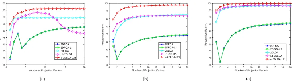
Figure11. Average classification accuracy versus the projection vectors number of different methods on three databases. (a) AR, (b)Exp1-2 on the Extended Yale B, (c)Exp1-2 on the CMU PIE.

convergence. Table III illustrates that our method is faster than the other LDA-based methods, but slightly slower than the other three comparison algorithms. The reason may be that all LDA-based methods including ours need to iteratively solve the projection vectors, but our method converges very quickly.

C. Experiments for 2-D methods

In this section, we do the same experiments as those for the 1-D methods in the Extended Yale B, AR, and CMU PIE databases to validate e-2DLDA-L21, and compare with some two-dimensional methods. Tables VIII, IX and VII list the av-erage recognition accuracy of each method and corresponding standard deviation (Std) on the Extended Yale B, CMU PIE and AR databases, respectively. Figure 11 plots the average classification accuracy of each approach versus the number projection vectors, and Figure 12 shows the convergence curve of e-2DLDA-L21 in these databases.

TABLE VII

CORRESPONDING STANDARD DEVIATION(STD)ON THEARDATABASE.

Methods accuracy std

e-2DLDA-L21 96.08 0.60

2DPCA 82.71 0.94

2DPCA-L1 82.72 0.95

2DLDA 89.93 0.68

L1-2DLDA 94.22 0.79

As can be seen in the aforementioned experimental results for tow-dimensional methods, we have that

• Discriminant methods are consistently superior to

2DPCA and 2DPCA-L1. This is probably because that 2DPCA and 2DPCA-L1 are unsupervised and do not well encode the discriminant information. L1-2DLDA is overall superior to traditional 2DLDA. The reason is that `1-norm is robust to outliers, compared with squared`2

-norm. However, 2DLDA is superior to L1-2DLDA in some experiments. This is probably because that L1-2DLDA does not relate to scatter matrices that well characterize geometric structure of data, while 2DLDA does.

TABLE VIII

CORRESPONDING STANDARD DEVIATION(%)ON THEEXTENDEDYALEB

DATABASES

e-2DLDA-L21 98.03±0.29 97.69±0.30 97.77±0.30 94.34±0.59

2DPCA 55.64±1.44 58.33±0.69 51.58±0.80 51.48±0.85 2DPCA-L1 53.77±1.07 59.44±0.60 51.61±0.72 51.43±0.88 2DLDA 81.81±0.56 85.41±0.55 85.16±1.18 84.71±1.11 L1-2DLDA 82.25±0.52 84.70±0.46 83.54±1.08 81.42±1.23

TABLE IX

CORRESPONDING STANDARD DEVIATION(%)ON THECMU PIE

DATABASES

e-2DLDA-L21 99.94±0.15 99.71±0.11 99.99±0.02 97.30±0.21

2DPCA 77.58±0.45 85.09±0.72 77.54±1.49 76.50±1.58 2DPCA-L1 79.09±0.50 85.61±0.57 77.38±1.49 76.50±1.59 2DLDA 97.49±0.72 98.59±0.30 99.11±0.57 95.78±0.67 L1-2DLDA 99.20±0.42 98.42±0.30 99.24±0.47 95.24±0.68

• Our approache-2DLDA-L21 is superior to the other two-dimensional methods. This is probably because that our method well reveals nonlinear features and discriminant features by Euler transform and`2,1-norm. Another

rea-son is that our method relates to scatter matrices and well exploits geometric structure of data. Figure 12 shows that our proposed algorithm monotonically decreases the value of the objective function and has a good conver-gence.

[image:11.612.61.551.65.204.2]

(12)

0 10 20 30 40 50 60 70 80 90 100 Number of Iteration

4.1 4.15 4.2 4.25 4.3 4.35 4.4 4.45 4.5

Objective Fuction Value (log10)

AR Extended Yale B CMU PIE

Figure12. Convergence curves ofe-2DLDA-L21 on three databases.

TABLE X

THE AVERAGE CLASSIFICATION ACCURACY(%)AND CORRESPONDING

STANDARD DEVIATION(%)ON THEEXTENDEDYALEBDATASET

e-LDA-L21 90.10±0.69 87.90±0.77 90.40±0.62 87.49±1.12

LDA-L21 87.94±0.62 86.58±0.67 87.73±0.72 84.40±1.12

e-LDA-L1 84.58±0.89 84.23±0.97 82.53±0.91 80.36±0.87

LDA-L1 69.99±2.47 71.12±2.04 67.53±6.53 68.12±6.41

other datasets, two-dimensional methods are inferior to the corresponding 1D discriminant methods. The reason may be that two-dimensional methods would be con-fronted with the heteroscedastic problem and the problem would be more serious for two-dimensional methods than the one for 1D-dimensional methods [52].

D. Discussion

1) : `2,1-norm and Euler transform

To discuss the effects of Euler transform and `2,1-norm for

discriminant analysis respectively, we compared e-LDA-L1,

e-LDA-L21, LDA-L1 and LDA-L21 on the Extended Yale B, LFWcrop and SUFR-W databases. In the experiments, we selected the aforementioned training images and corre-sponding testing images on these datasets. Tables X and XI list the average recognition accuracy of each approach and corresponding standard deviation (Std), respectively. Figure 13 plots the average classification accuracy of each approach versus the number projection vectors on the Extended Yale B, LFWcrop and SUFR-W databases, respectively.

• Discriminant methods with Euler transformation (e-

LDA-L21 and e-LDA-L1) are superior to the corresponding methods without Euler transformation (LDA-L21 and LDA-L1). The reason may be that e-LDA-L21 and

e-LDA-L1 calculate the dissimilarity and similarity be-tween data in the Euler space which can suppress outliers and reveal nonlinear features. Moreover, Euler space can help improve the separability of data and obtain a large margin for different classes.

TABLE XI

THE AVERAGE CLASSIFICATION ACCURACY(%)AND CORRESPONDING

STANDARD DEVIATION(%)ON THELFWCROP ANDSUFR-WDATASETS

Methods LFWcrop SUFR-W

accuracy std accuracy std

e-LDA-L21 54.55 3.33 40.11 2.60

LDA-L21 45.18 1.77 33.44 1.81

e-LDA-L1 49.08 1.48 39.85 2.53

LDA-L1 28.58 2.79 24.67 2.02

• Methods, which employ `2,1-norm as distance metric,

are superior to `1-norm based methods. The reason is

that `2,1-norm based methods reveal within-class and

between-class scatters, while `1-norm based methods

do not. Moreover, `2,1-norm enlarges the role of small

between-class distance. This helps get a large margin which is important for classification. However, it is un-clear whether `1-norm plays the same role.

• Table XI shows that LDA-L21 is inferior to e-LDA-L1. The reason may be that LDA-L21 does not well encode nonlinear discriminant features. It also illustrates that Euler transform well revels nonlinear features.

• Figure 13 illustrates that e-LDA-L21 is superior to the

other three methods and obtains the best recognition accuracy among the four methods under the same number of projection vectors.

2) : The sensitivity analysis of the parameterα.

In order to well illustrate the influence of parameterαin our model, we added some experiments on the Extended Yale B, AR and SUFR-W databases. In the experiments, we selected the aforementioned training images and corresponding testing images on these datasets. Figure 14 plots the curves of classification accuracy versus parameterαon three databases, respectively, and also marks the maximum value for each group experiments.

• From Figure 14 (a), we can see that α has a large influence for the classification accuracy of our method under the different group experiments on the Extend Yale B database. It is unable to select the same α in this dataset. Thus, we select different α for different group experiments on the Extended Yale B dataset.

• Figure 14 (b) illustrates that α has little influence for the classification accuracy of our method on the AR and SUFR-W databases. Whenαis in [0.9 1.1] interval, our method overall has good performance. Thus, we setαas 1.0 in the experiments on the AR and SUFR-W datasets.

VI. CONCLUSION

We present a robust supervised approach, namely Euler LDA-L21(e-LDA-L21), for dimensionality reduction.e- LDA-L21 maps image onto Euler space and employs `2,1-norm

[image:12.612.338.529.92.172.2]

(13)

0 5 10 15 20 25 30 35 40

0 10 20 30 40 50 60 70 80 90

e-LDA-L21 LDA-L21 e-LDA-L1 LDA-L1

(a)

0 10 20 30 40 50 60

(b)

0 10 20 30 40 50 60

0 5 10 15 20 25 30 35 40

(c)

Figure13. Average classification accuracy versus the projection vectors number of different methods on three databases. (a)Exp2-2 on the Extended Yale B, (b)LFWcrop, (c)SUFR-W.

0.2 0.4 0.6 0.8 1 1.2 1.4 1.6 1.8

70 75 80 85 90 95

Exp1-1 Exp1-2 Exp2-1 Exp2-2

x : 0.7 y : 87.67

x : 0.7 y : 87.49 x : 0.1

y : 90.10

x :0.3 y : 90.40

(a)

0.1 0.3 0.5 0.7 0.9 1.1 1.3 1.5 1.7 1.9

95 96 97 98 99 100

AR

0.1 0.3 0.5 0.7 0.9 1.1 1.3 1.5 1.7 1.9

30 35 40 45 50

SUFR-W

x : 0.9 y : 98.19

x : 1.1 y : 40.56

(b)

Figure14. The curve of classification accuracy versus the parameterα. (a) Extended Yale B, (b)AR and SUFR-W.

space to an explicit Euler feature space and does not in-crease the dimensionality of features, while kernel LDA does not. Compared with most existing robust LDA methods, our method not only is robust to outliers but also helps obtain a large margin in the low-dimensional space. Thus, our method encodes discriminant information. Experiment results illustrate that our proposed algorithms have a good convergence and our methods are superior to the other robust methods for image classification.

For feature extraction, rotational invariance is one of the important properties [50] [51]. As the aforementioned anal-ysis, from the norm point of view, `2,1-norm and traditional

squared`2-norm have no essential difference, thus, our method

retains traditional LDA’s rotation invariance. We will study this problem in future work.

ACKNOWLEDGMENT

The authors would like to thank the anonymous reviewers and AE for their constructive comments and suggestions, which improved the paper substantially. We also thank Prof. X. Gao for polishing our paper. Finally, we wold like to thank Prof. S. Liao and Dr. Zhang for providing the codes of XQDA and DNS.

REFERENCES

[1] M. Turk and A. Pentland, ”Eigenfaces for recognition”, J. Cognitive

Neurosci., vol. 3, no. 7, pp. 71-86, winter. 1991.

[2] P. N. Belhumeur, J. Hespanha and D. J. Kriegman, ”Eigenfaces vs. Fisherfaces: recognition using class specific linear projection”, IEEE

Trans. Pattern Anal. Mach. Intell., vol. 19, no. 7, pp. 711-720, Jul. 1997.

[3] Jian Yang, D. Zhang, A. F. Frangi and Jing-yu Yang, ”Two-dimensional PCA: a new approach to appearance-based face representation and recognition”,IEEE Trans. Pattern Anal. Mach. Intell., vol. 26, no. 1, pp. 131-137, Jan. 2004.

[4] H. Lu, K. Plataniotis and A. Venetsanopoulos, ”MPCA: Multilinear principal component analysis of tensor objects”, IEEE Trans. Neural

Netw., vol. 19, no. 1, pp. 8-39, Jan. 2008.

[5] J. Yang, D. Zhang, Y. Xu and J. Yang, ”Two-dimensional discriminant transform for face recognition”, Pattern Recognit., vol. 38, no. 7, pp. 1125-1129, Jul. 2005.

[6] J. Ye, J. Ravi Janardan and L. Qi, ”Two-dimensional linear discriminant analysis”,In proc. Advances in Neural Information Processing Systems, pp. 1569-1576, 2005.

[7] L. Zhang, Q. Gao and D. Zhang, ”Directional independent component analysis with tensor representation”,Proc. IEEE Int. Computer Vision

and Pattern Recogni., pp. 1-7, 2008.

[8] Q. Gao, F. Gao, H. Zhang, X. Hao, and X. Wang, ”Two-dimensional maximum local variation based on image Euclidean distance for face recognition”,IEEE Trans. Image Processing, vol. 22, no. 10, pp.3807-3817, 2013.

(14)

[10] P. Roth, P. Wohlhart, and M. Hizer, ”Large Scale Metric Learinng from Equivalence Constraints”, IEEE Conference on Computer Vision and

Pattern Recognition, pp. 2288-2295, 2012.

[11] N. Martinel, C. Micheloni, G. L. Foresti, ”Kernelized Saliency-based Person Re-Identification through Multiple Metric Learning”, IEEE

Transactions on Image Processing, vol. 24, no.12, pp. 5645-5658, 2015.

[12] Z. Li, S.Chang, F. Liang, T.S. Huang, L. Cao, and J.R. Smith,”Learning locally-adaptive decision functions for person verification”,Computer

Vision and Pattern Recognition, vol. 9 no. 4 pp. 3610-3617, 2013.

[13] S. Liao, Y. Hu, X. Zhu, ”Person Re-identification by Local Maximal Occurrence Representation and Metric Learning”,IEEE Conference on

Computer Vision and Pattern Recognition, vol. 8, no. 4, pp. 2197-2206,

2015.

[14] S. Liao , Z. Li, ”Efficient PSD Constrained Asymmetric Metric Learning for Person Re-Identification”,IEEE International Conference on

Com-puter Vision pp. 3685-3693, 2015.

[15] L. Zhang, T. Xiang, and S.Gong, ”Learning a Discriminative Null Space for Person Re-identification”,IEEE Conference on Computer Vision and

Pattern Recognition, pp:1239-1248, 2016.

[16] N. Martinel, A. Das, C. Micheloni, and A. Roy-Chowdhury, ”Temporal model adaptation for person re-identification”,European Conference on

Computer Vision(ECCV), pp. 858-877, 2016.

[17] X. Zhu, X. Jing, F. Wu, and H. Feng, ”Video-based person re-identification by simultaneously learning intra-video and inter-video dis-tance metrics”,International Joint Conference on Artificial Intelligence, pp:3552-3558,2016.

[18] L. Luo, J. Yang, J. Qian, T. Ying, and G. Lu, ”Robust image regression based on the extended matrix variate power exponential distribution of dependent noise”,IEEE Transactions on Neural Networks and Learning

Systems, vol. 28, no. 9, pp. 2168-2182, 2017.

[19] Z. Zhang, F. Li, M. Zhao, L. Zhang and S. Yan, ”Robust Neighborhood Preserving Projection by Nuclear/L2,1-Norm Regularization for Image Feature Extraction”,IEEE Trans. on Image Processing, vol. 26, no. 4, pp. 1607-1622, 2017.

[20] Q. Ke and T. Kanade, ”Robust L1 norm factorization in the presence of outliers and missing data by alternative convex programming”,Proc.

IEEE Int. Computer Vision and Pattern Recogni., pp. 592-599, 2005.

[21] N. Kwak, ”Principal component analysis based on L1-norm maximiza-tion”,IEEE Trans. Pattern Anal. Mach. Intell., vol. 30, no. 9, Jun. 2008. [22] X. Li, Y. Pang and Y. Yuan, ”L1-norm-based 2DPCA”, IEEE Trans.

Syst., Man, Cybern. B, Cybern., vol. 40, no. 4, pp. 1170-1175, Jan.

2010.

[23] F. Nie, H. Wang, C. H. Ding, D. Luo and H. Huang, ”Robust principal component analysis with non-Greedy l1-Norm maximization”,Proc. Int.

Joint Conf. Artificial Intelligence, pp. 1433-1438, 2011.

[24] R. Wang, F. Nie, X. Yang, F. Gao and M. Yao, ”Robust 2DPCA with non-greedy L1-norm maximization for image analysis”,IEEE Trans.

Cybernetics, vol. 45, no. 5, pp. 1108-1112, May. 2015.

[25] N. Kwak, ”Principal Component Analysis by Lp-Norm Maximization”,

IEEE Trans. on Cybern., vol. 44, no. 5, pp. 594-609, Apri. 2014.

[26] F. Zhang, J. Yang, J. Qian and Y. Xu, ”Nuclear norm-based 2-DPCA for extracting features from images”,IEEE Trans. Neural Networks and

Learning Systems, Vol. 26, no. 10, pp. 2247-2260, Oct. 2015.

[27] H. Wang, F. Nie and H. Huang, ”Robust distance metric learning via simultaneous L1-norm minimization and maximization”,Proc. Int. Conf.

Mach. Learn., pp. 1836-1844, 2014.

[28] F. Zhong and J. Zhang, ”Linear discriminant analysis based on L1-norm maximization”,IEEE Trans. Image Processing, vol. 22, no. 8, pp. 3018-3027, Aug. 2013.

[29] W. Zheng, Z. Lin and H. Wang, ”L1-Norm kernel discriminant analysis via Bayes error bound optimization for robust feature extraction”,IEEE

Trans. Neural Netw. Learn. Syst., vol. 25, no. 4, pp. 793-805, Apr. 2014.

[30] X. Chen, J. Yang and Z. Jin, ”An improved linear discriminant analysis with L1-norm for robust feature extraction”,Proc. Int. Conf. Pattern

Recogni., pp. 1585-1590, 2014.

[31] Y. Liu, Q. Gao, S. Miao, X. Gao, F. Nie, and Y. Li, A non-greedy algorithm for L1-norm LDA,IEEE Trans. Image Processing, vol. 26, no. 2, pp. 684-695, 2017.

[32] Q. Wang, Q. Gao, D. Xie, X. Gao, and Y. Wang, ”Robust DLPP With Nongreedy L1-Norm Minimization and Maximization”,IEEE Trans. on

Neural Networks and Learning Systems, vol. 29. no. 3, pp. 738-743,

2018.

[33] C. Li, Y. Shao and N. Deng, ”Robust L1-norm two-dimensional linear discriminant analysis”,Neural Networks, vol. 65, pp. 92-104, May. 2015. [34] Q. Gao, L. Ma, Y. Liu, X. Gao, F. Nie, ”Angle 2DPCA: a new formulation for 2DPCA”,IEEE Transactions on Cybernetics, vol. 48, no. 5, pp. 1672-1678, 2018.

[35] C. Ding, D. Zhou, X. He and H. Zha, ”R1-PCA: rotational invariant L1-norm principal component analysis for robust subspace factorization”,

Proc. Int. Conf. Mach. Learn., pp. 281-288, 2006.

[36] Q. Wang, Q, Gao, X.Gao, and F. Nie, ”Optimal mean two-dimensional principal component analysis with F-norm minimization”,Pattern

recog-nition, vol. 68, pp. 286-294, 2017.

[37] J. Gui, D. Tao, Z. Sun, Y. Luo, X. You and Y. Tang, ”Group sparse multiview patch alignment framework with view consistency for image classification”,IEEE Trans. Image Process., vol. 23, no. 7, pp. 3126-3137, Jul. 2014.

[38] F. Nie, H. Huang, X. Cai and C. Ding, ”Efficient and robust feature selection via joint L2,1-norms minimization”, Advances in Neural

In-formation Processing Systems, pp. 1813-1821, 2010.

[39] X. Shi, Y. Yang, Z. Guo and Z. Lai, ”Face recognition by sparse dis-criminant analysis via joint L2,1-norm minimization”,Pattern Recognit., vol. 47, pp. 2447-2453, Jul. 2014.

[40] W. Wong, Z. Lai, Y. Xu, J. Wen and C. Ho, ”Joint tensor feature analysis for visual object recognition”,IEEE Trans. Cybernetics, vol. 45, no. 11, pp. 2425-2436, Nov. 2015.

[41] C. Hou, F. Nie, D. Yi and Y. Wu, ”Feature selection via joint embedding learing and sparse regression”,Proc. 22nd Int. Joint Conf. Artif. Intell., pp. 1324-1329, 2011.

[42] A. J. Fitch, A. Kadyrov, W. J. Christmas, and J. Kittler, ”Fast robust correlation”,IEEE Trans. Image Processing, vol. 14, no. 8, pp. 1063-1073, 2005.

[43] S. Liwicki, G. Tzimiropoulos, S. Zafeiriou, and M. Pantic, ”Euler prin-cipal component analysis”,International Journal of Computer Vision, vol. 101, no. 3, pp. 498-518, 2013

[44] M. H. Nguyen and F. Torre, ”Robust kernel principal component analysis”,In Advances in Neural Information Processing Systems, pp. 1185C1192, 2009.

[45] Fukunaga K,Introduction to statistical pattern recognition, Academic press, 2013.

[46] A. S. Georghiades, P. N. Belhumeur and D. J. Kriegman, ”From few to many: illumination cone models for face recognition under variable lighting and pose”,IEEE Trans. Pattern Anal. Mach. Intell., vol. 23, no. 6, pp. 643-660, Jun. 2001.

[47] A. M. Martinez, ”The AR face database”, CVC Technical Report, 24, 1998.

[48] T. Sim, S. Baker and M. Bsat, ”The CMU Pose, Illumination, and Expression (PIE) database”, Proceedings of Fifth IEEE International

Conference on Automatic Face Gesture Recognition, Washington, DC,

pp. 46-51, 2002.

[49] J. Leibo, Q. Liao, T. Poggio, ”Subtasks of unconstrained face recogni-tion”,VISAPP, vol. 2, pp. 113-121, 2014.

[50] C. Sanderson and B. C. Lovell, ”Multi-region probabilistic histograms for robust and scalable identity inference”,Proc. Int. Conf. Biometrics, pp.199-208, 2009.

[51] Q. Liao, J. Leibo, and T. Poggio, ”Learning invariant representations and applications to face verification”,proc. Advances in Neural Information

Processing Systems, pp. 3057-3065, 2013.

[52] W. Zheng, J. Lai, and Stan Z. Li, ”1D-LDA vs. 2D-LDA: When is vector-based linear discriminant analysis better than matrix-vector-based?” Pattern

Recognition, vol. 41, no. 7, pp. 2156-2172, 2008.

(15)

Quanxue Gao received the B. Eng. degree from xi’an Highway University, Xi’an, China, in 1998, the M.S. degree from the Gansu University of Technol-ogy, Lanzhou, China,in 2001, and the Ph.D. degree from Northwestern Polytechnical University, Xi’an China, in 2005. He was a associate research with the Biometrics Center, The Hong Kong Polytechnic University, Hong Kong from 2006 to 2007. From 2015 to 2016, he was a visiting scholar with the department of computer science, The University of Texas at Arlington, Arlington USA. He is currently a professor with the School of Telecommunications Engineering, Xidian University, and also a key member of State Key Laboratory of Integrated Services Networks. He has authored 40 technical articles in refereed journals and proceedings, including IEEE Transactions on Image Processing, IEEE Transactions on Neural Networks and Learning Systems, IEEE Transactions on Cybernetics, CVPR, AAAI, and IJCAI. His current research interests include pattern recognition and machine learning.

Zhaohua Yangreceived the B.S. degree in precision instruments and machinery from Harbin Institute of Technology, Harbin, China, in 1998, the M.S. degree in control theory and engineering from Lanzhou University of Technology, Lanzhou, China, in 2001, and the Ph.D. degree in precision instruments and machinery from Harbin Institute of Technology in 2004. She was Visiting scholar from Washington University in St. Louis in 2012. She is currently an Associate Professor in the School of Instrumentation Science and Opto-electronics Engineering, Beihang University, Beijing, China. She has authored 50 technical articles in refereed journals and proceedings including IEEE Transactions on Industrial Electron-icsInstrument and Measurement and etc. Her current research interests include ghost imaging, Pattern recognition, and engineering applications.

Fang Chenreceived the B. Eng. Degree in Commu-nication Engineering from Lanzhou Jiaotong Uni-versity, China, in 2014. She is currently a M.S. degree candidate in traffic information engineer-ing and control in Xidian University, China. Her research interests include pattern recognition, and dimensionality reduction and face recognition.

Feiping Nie received the Ph.D.degree in computer science from Tsinghua University, Beijing,China, in 2009. He was respectively a Post Doctoral Research Associate, Research Assistant Professor,and Research Professor with the University of Texas at Arlington, Arlington, TX,USA, from 2009 to 2015.He is currently a professor of Northwestern Polytechnical University, Xi’an China. He has authored 160 technical articles in refereed journals and proceedings, including IEEE Trans. on Pattern Analysis and Machine Intelligence,International Journal of Computer Vision, IEEE Trans. on Image Processing, IEEE Trans. Neural Networks and Learning Systems, IEEE Trans.Cybernetics, IEEE Trans. Knowledge and Data Engineering, ICCV, CVPR, ICML, AAAI, IJCAI, and NIPS. His current research interests include machine learning and its application fields, such as pattern recognition, data mining,computer vision,image processing, and information retrieval.