New developments in the CAPTAIN
Toolbox for Matlab with case study
examples
?
C. J. Taylor∗ P. C. Young∗∗ W. Tych∗∗∗ E. D. Wilson∗
∗Engineering Department, Lancaster University, UK
(e-mail: [email protected], [email protected]) ∗∗Lancaster Environment Centre, Lancaster University, UK; Fenner
School of Environment and Society, Australian National University, Canberra; Australia (e-mail: [email protected]) ∗∗∗Lancaster Environment Centre, Lancaster University, UK
(e-mail: [email protected])
Abstract: The CAPTAIN Toolbox is a collection of Matlab algorithmic routines for time series analysis, forecasting and control. It is intended for system identification, signal extraction, interpolation, forecasting and control of a wide range of linear and non–linear stochastic systems across science, engineering and the social sciences. This article briefly reviews the main features of the Toolbox, outlines some recent developments and presents a number of examples that demonstrate the performance of these new routines. The examples range from consideration of global climate data, through to electro–mechanical systems and broiler chicken growth rates. The new version of the Toolbox consists of the following three modules that can be installed independently or together: off–line, time–varying parameter estimation routines forUnobserved Component (UC) modelling and forecasting; Refined Instrumental Variable (RIV) algorithms for the identification and estimation of both discrete and ‘hybrid’ continuous–time transfer
function models; and various routines forNon–Minimal State Space (NMSS) feedback control
system design. This new segmented approach is designed to provide new users with a gentler introduction to Toolbox functionality; one that focuses on their preferred application area. It will also facilitate more straightforward incorporation of novel algorithms in the future.
Keywords:Identification; estimation; forecasting; signal processing; control system design; robotic systems; climate data; chicken growth
1. INTRODUCTION
The Computer–Aided Program for Time Series Analysis and Identification of Noisy Systems (CAPTAIN) Toolbox provides access to novel algorithms for various important aspects of system identification, estimation, nonstationary time series analysis, signal processing, adaptive forecasting and automatic control system design. These algorithms have been developed by the first three authors of this article, and their colleagues (see Acknowledgements), over many years. In fact, CAPTAIN was originated by the second author over 40 years ago, whilst the first Matlab implementation was released in 2000 (Pedregal et al., 2007;
Taylor et al., 2007). The books on Recursive Estimation
and Time Series Analysis (Young, 2011) and True Digi-tal Control: Statistical Modelling and Non–Minimal State Space Design (Taylor et al., 2013) contain information on the history, derivation and use of all of the algorithms in the Toolbox.
? This work is supported by the Engineering and Physical Sciences
Research Council (EPSRC), EP/M015637/1 and EP/R02572X/1; and project Programa Estatal de Investigacion 2013–2016, Spain (ECO2015–70331–C2–1–R).
In essence, the Toolbox represents the output of various on–going investigations into Matlab implementations of the underlying algorithms, as well as default and optional values of the input parameters to the routines. This should help both expert and less experienced modellers to use these routines when they are considering the analysis of data sets across a wide range of scientific disciplines, as illustrated by the citations to e.g. Taylor et al. (2007) that have appeared in diverse areas of the open literature.
As explained later in the article, the latest version of the Toolbox includes improved routines and new modelling tools. Furthermore, the Toolbox has recently been reorgan-ised significantly and now consists of the following three distinct modules:
(1) TVPMOD: Time Variable Parameter (TVP) MODels. For the identification of Unobserved Com-ponent (UC) models, with a particular focus on time–variable and state–dependent parameter
mod-els, including the popular Dynamic Harmonic
(2) RIVSID: Refined Instrumental Variable (RIV) System Identification algorithms. For optimal RIV identification of multiple–input, continuous and
discrete–time,Transfer Function (TF) models.
(3) TDCONT: True Digital CONTrol (TDC). For multivariable control, including pole assignment and optimal LQ/LQG (Linear–Quadratic–Gaussian) de-sign, and with both backward shift (z−1) and delta– operator (δ) options.
A web site http://captaintoolbox.co.uk is devoted to the
Toolbox: it reports recent developments, as well as pro-viding short discussions on technical issues arising. The Toolbox is free to non–commercial users and can be down-loaded from:http://www.lancaster.ac.uk/staff/taylorcj/tdc.
The present article reviews the main features of the Tool-box (section 2); outlines some recent improvements and a number of other developments that will be added in the future (section 3); and presents a number of examples that demonstrate its practical application (section 4). These examples include the analysis of global climate models and paleo–climatic data, a nonlinear electro–mechanical system, and broiler chicken growth curves. The article refers to a rather large number of acronyms, the most important of which are summarised in Table 1.
2. CAPTAIN TOOLBOX OVERVIEW
The CAPTAIN Toolbox has evolved to service the
require-ments of the Data–Based Mechanistic (DBM) modelling
philosophy (see e.g. Young, 1978, 2011; Price et al., 1999). DBM models are obtained initially from the analysis of observational time–series but are only considered credible if they can be interpreted in physically meaningful terms. It is a philosophy that emphasises the importance of para-metrically efficient, low order, dominant mode models, as well as the development of stochastic methods and the as-sociated statistical analysis required for the identification and estimation of such models. It stresses the importance of explicitly acknowledging the basic uncertainty that is essential to the characterisation of any physical, chemical, biological or socio-economic process.
2.1 Toolbox Structure
The TVPMOD module is based around a state–space framework that allows for the identification of UC models. Here, the time series is assumed to be composed of an addi-tive or multiplicaaddi-tive combination of different components that have defined statistical characteristics but which can-not be observed directly. The stochastic evolution of each parameter is assumed to be described by a generalised ran-dom walk process. The TVP estimates are obtained first from a forward pass Kalman filtering step that also allows for forecasting from the end of the time series. However, because the estimates on this forward pass are lagged, as a result of the filtering operations, optional updating, using a
backwards–recursive, Fixed Interval Smoothingalgorithm
yields lag–free estimates and allows for signal extraction, interpolation over gaps in the time series and backcasting.
In this manner, TVPMOD provides routines for the
optimal estimation of dynamic (i.e. TVP) regression
mod-Table 1. Abbreviations.
TVPMOD Time Variable Parameter module
RIVSID System Identification module
TDCONT True Digital Control module
ARX Auto–Regression with eXogenous variables
CT Continuous–Time
DBM Data–Based Mechanistic
DHR Dynamic Harmonic Regression
DT Discrete–Time
MPC Model Predictive Control
NMSS Non–Minimal State Space
PIP Proportional–Integral–Plus
RIV Refined Instrumental Variable
RIVBJ RIV for full Box–Jenkins models
SDP State Dependent Parameter
TDC True Digital Control
TF Transfer Function
TVP Time Variable Parameter
UC Unobserved Components
els, including linear regression; auto–regression, which is useful for spectrogram estimation (Young, 2006); and DHR (Young et al., 1999), which provides a very powerful forecasting algorithm (see the examples in section 4.1
and 4.4). Finally, a closely related algorithm for State
Dependent Parameter (SDP) estimation provides a non– parametric identification procedure for a wide class of nonlinear and chaotic systems (see section 4.2).
The RIVSID module includes routines for the optimal identification and estimation of a unified Box–Jenkins model that includes both discrete and continuous–time TF models (Young, 2011, 2015; Taylor et al., 2013). One advantage of such TF models is their simplicity and ability to characterise the dominant modal behaviour of a stochastic, dynamic system. This makes such a model an ideal basis for control system design, model reduction and large simulation model emulation (Taylor and Shaban, 2006; Young and Ratto, 2011).
Finally, with the newTDCONTmodule (see section 3.2),
the latest version of the Toolbox now has a full set of algorithms for control system design, simulation and robustness evaluation (Taylor et al., 2013).
2.2 How to use the Toolbox
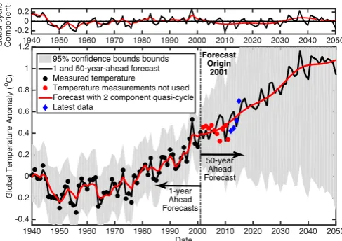
The Toolbox is primarily used by means of standard func-tion calls i.e. directly from the Matlab Command Window or from scripts. Each function is called using a number of input and output arguments. Here, default input argu-ments are embedded into CAPTAIN and usually provide a reasonable initial result, while the full power of the Toolbox is accessed through the wide range of optional settings. For example, a smoothed trendysfor the climate data illustrated in Fig. 1 (see later) is straightforwardly
obtained using ys = irwsm(y), in which irwsm is a
CAP-TAIN function for the estimation of integrated random walk models. There is only one input argument, the data
y, and so CAPTAIN utilises the most typical model for this type of analysis. However, enteringys = irwsm(y,TVP,nvr)
Finally, the Toolbox includes over 50 useful command line demos. These illustrate the wide scope of models and algo-rithms. Experience suggests that one of the most effective ways to get started with CAPTAIN is to examine such demos and then to adapt them for each new data set of interest, so saving much time in algorithmic development.
3. RECENT DEVELOPMENTS
Earlier articles about the Toolbox, presented in software–
themed sessions at the IFAC System Identification
se-ries of conferences, have included Young et al. (2009) and Young and Taylor (2012). The first of these provides an overview of its functionality, with practical examples based on the Mauna Loa atmospheric carbon dioxide series and flow data for the River Canning in Western Australia. The second reported on new functions for the estimation of multiple–input TF models with different denominator polynomials and on some improvements for real–time recursive estimation, with a practical example concerning the Leaf River catchment in Mississippi, USA. The following discussion focuses on the main developments subsequent to these and describes some new examples. The Toolbox has also been updated in various other minor ways during the past few years, not least to fix bugs and to ensure compatibility with the latest versions of Matlab.
3.1 New Modular Structure
In recent years, the Toolbox has grown to over 300 rou-tines, sometimes leading to confusion, especially for new users who might not know where to start. Hence, one re-cent development is the introduction of the three modules noted above. In addition to the superficial division of the Toolbox into three separate folders, the reorganisation is accompanied by revisions to the user help information, the development of new demos for each module, and the preparation of three new user handbooks (in–progress). In addition, some of the common sub–functions (not normally directly called by the user) have been rewritten to ensure that each module can operate independently of each other. These new arrangements are primarily designed to help the Toolbox developers to more rapidly correct bugs, and to upgrade with new algorithms in the future. However, further work is required to continue to improve the ac-cessibility of the Toolbox, particularly for inexperienced users. Many functions in the Toolbox include an enormous number of options. These provide value to the authors and a small number of other users, but can seem overly complicated to occasional modellers, hence a streamlining of some of the options is now in progress.
3.2 New TDCONT Module
In contrast to some other Matlab toolboxes that focus on
either system identification or control, CAPTAIN
facili-tates an integrated TDC approach that encompasses the entire design process, from data–based model identifica-tion, through to control system design and implementa-tion, using a digital, sampled–data standpoint through-out (Taylor et al., 2013). In brief, the design procedure consists of (i) stochastic identification and recursive esti-mation of suitable control models (using RIVSID) based
on the analysis of either planned or monitored experimen-tal data; or via model reduction from data generated by a physically–based simulation model; (ii) off–line control algorithm design and initial evaluation (using TDCONT), via an iterative application of an appropriate discrete–time design methodology, coupled with closed–loop sensitivity analysis based on Monte–Carlo simulation; and (iii) imple-mentation and evaluation for the real process.
With regard to (iii), standard real–time Matlab tools or other software environments can be utilised.
Alterna-tively, since the approach yields Proportional–Integral–
Plus(PIP) algorithms that can be interpreted as a logical extension of conventional PI/PID methods, it is usually straightforward to express the controller in a suitable in-cremental form, and hence implement using existing indus-try hardware–software frameworks. As a result, CAPTAIN Toolbox algorithms have been utilised for the design of PIP control systems in various practical domains, from agriculture (Lees et al., 1998; Taylor et al., 2000, 2004), robotics in construction (Shaban et al., 2008) and nuclear decommissioning (Taylor and Robertson, 2013) (see also section 4.2), as well as for simulation–based research into e.g. engines (Jamali et al., 2015).
Central to TDCONT is a generalisedNon–Minimal State
Space (NMSS) model that allows for deterministic and stochastic optimal control design, in addition to pole as-signment and predictive control options. In contrast to earlier versions of the Toolbox, the new module includes delta–operator design (Chotai et al., 1998), robustness evaluation (Taylor et al., 2001) and analytical multivari-able decoupling; and the authors are presently adding functions for nonlinear control based on SDP models. Furthermore, the included demos reproduce almost every worked example and graphical output from a complemen-tary book on state–space control (Taylor et al., 2013). In other words, NMSS feedback is utilised in TDCONT as a unifying framework for generalised digital control system design, with the included demos providing a relatively gentle learning curve, from which potentially challenging topics, such as optimal, stochastic and multivariable con-trol can all be investigated.
3.3 Other Algorithmic Developments
The major up–coming changes to CAPTAIN are a new
routine for Multi–State Dependent Parameter (MSDP)
estimation; an Arbitrary Sampling DHR (ASDHR)
algo-rithm that allows for non–uniformly sampled data; modi-fications to the RIVSID routines to allow for more refined initiation on the very few occasions when the standard pro-cedures might fail, as well as automating the present advice about estimating initial conditions when usingrivcbj (out-lined in http://captaintoolbox.co.uk/Captain_Toolbox.html/ Technical_Matters/Technical_Matters.html); and, finally, mak-ing the input and output arguments of routines conform better with those of other well–known toolboxes, such as SID and CONTSID (Padilla et al., 2015).
this using high order ARX modelling and emulation but additional changes in the future are intended to automate the procedure completely.
4. ILLUSTRATIVE EXAMPLES
The first two examples exploit Continuous–Time (CT) models. CAPTAIN was the first Matlab Toolbox to allow for optimal identification of both Discrete–Time (DT) and CT models from sampled data in a unified ‘hybrid’ TF form (Young, 2011), based on algorithms developed originally by Young and Jakeman (1979–1980). The latest versions of the CT routines (rivcbjid/rivcbj) are used in the first example, where they are combined with DHR modelling (dhr) for an important forecasting application.
The second example utilises rivcbj and sdp for a robotic
system. Further examples demonstrate DT estimation (using rivbjid/rivbj) for a biological control problem and application ofdhrto a noisy paleo–climatic data set.
4.1 Global Climate Model Identification and Forecasting
This recent study (Young, 2018) follows from earlier work on climate modelling and carbon emissions management (Jarvis et al., 2009). It is based on a UC model and has involved rivcbjid/rivcbj modelling of the continuous– time TF relationship between total radiative forcing and the globally averaged surface temperature; together with
dhr modelling of an additive, quasi–cyclic component.
This component plays an important part in explaining the temperature changes and appears to be related to other quasi–cyclic climate phenomena, such as theAtlantic Multidecadal Oscillation (AMO). The complete model forms the basis for forecasting using the Kalman filter that is part of the DHR algorithm. A typical example is shown in Fig. 1, where we see that, on the basis of only the data up to 2001, it is able to forecast successfully the changes in the global temperature for 15 years ahead and produce forecasts after this which seem feasible. The CT model is important because it is related directly to the differential equation models used by climate scientists and is characterised by parameters that can be interpreted directly in climate terms. Also, therivcbjroutine yields low order CT models that are able to ‘emulate’ the response of large climate models almost perfectly.
4.2 Nonlinear Electro–Mechanical System Identification
This example is also based on CT modelling, this time
a differential equation model of a nonlinear
Electro-Mechanical Positioning System (EMPS), where the sdp
implementation of the SDP algorithm is used to identify frictional nonlinearity in the system. This routine exploits fixed interval smoothing, together with special re–ordering of the data to generate a non–parametric (graphical) es-timate of the nonlinearity. First, thesdp routine provides the non–parametric estimate; then a suitable parametric function is selected that is able to characterise the shape of this estimate, with its parameters optimised using the
standard lsqnonlin optimisation routine in Matlab. Both
estimates are shown in Fig. 2 and it will be noted that the nonlinearity is identified as being asymmetrical. This is important in practical terms because it is normally
Date
1940 1950 1960 1970 1980 1990 2000 2010 2020 2030 2040 2050
Global Temperature Anomaly (
oC)
-0.4 -0.2 0 0.2 0.4 0.6 0.8 1 1.2
95% confidence bounds bounds 1 and 50-year-ahead forecast Measured temperature
Temperature measurements not used Forecast with 2 component quasi-cycle Latest data
1940 1950 1960 1970 1980 1990 2000 2010 2020 2030 2040 2050 Quasi-cyclic Component
-0.2 0 0.2
Forecast Origin
2001
[image:4.595.309.553.74.246.2]50-year Ahead Forecast 1-year Ahead Forecasts
Fig. 1. Global climate model: 50 year ahead forecast of global surface temperature from 2001.
Fig. 2. Electro–Mechanical System Identification showing SDP and Inverse Dynamic Model (IDM) estimates.
assumed to be symmetric and is estimated as such. The paper describing this study (Janot et al., 2017) also consid-ers nonlinear SDP control. This linearises the closed–loop system so that linear PIP control, exploiting the TDCONT routines and arivbj identified model of the inner closed– loop, is used for outer loop ‘trimming’ that refines the closed–loop response. Related SDP modelling and control approaches have been developed by Taylor and Robertson (2013) for a robotic hydraulic manipulator system.
4.3 Chicken Growth Curves
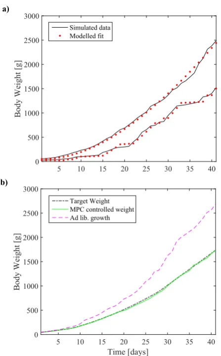
[image:4.595.308.553.292.483.2]Fig. 3. Simulated broiler chicken growth curves showing: a) modelling weight response to feed inputs and b) closed–loop controlled weight response.
libitum feed rule and an experimental feed rule. For the latter, each day the feed has a 50% of being the same as the ad libitum feed, or a 50% chance of being 20% of the ad libitum feed. The corresponding output growth is simulated using a nonlinear growth formula based on equation (5) from Aerts et al. (2003). From twenty–four simulated data sets, in twelve the feed was based on the ad libitum feed rule, and in the other twelve the experimental feed rule. Random variations to the inputs and output were added to the data. The best DT model structure across all data sets is identified. An example of the fit to two data sets is given in Fig. 3a. The average identified model parameters are used to design a constrained MPC. The resulting growth curve when using MPC is compared to ad libitum and the desired growth in Fig. 3b.
4.4 Detecting Long Term Cycles in Paleo–Climatic Data
The dhr routine has recently been used in the detection
and quantification of a millennial scale cycle in precip-itation changes, based on a high–resolution speleothem
δ18O record from northern Iberia (Smith et al., 2016).
These variations in precipitation delivery relate to an underlying millennial scale cycle in North Atlantic Os-cillation (NAO) dynamics, which show two distinct cycle lengths of approximately 1300 and 1500 years (extracted
Single cycle model periodicity
1200 1300 1400 1500 1600 1700 1800
Seasonal component norm
[image:5.595.319.541.70.251.2]0 1 2 3 4 5 6
Fig. 4. Total power measure (L2–norm of the modelled
cyclic component) of single periodicity against the tested periodicity range (years) (Smith et al., 2016).
time
0 2000 4000 6000 8000 10000 12000
detrended data and model's cycle components -0.8 -0.6 -0.4 -0.2 0 0.2 0.4 0.6
Dual period model R2=0.7379 Seasonal component norm: 10.5531
modelled harmonic components detrended data
Fig. 5. Full two cycles and trend DHR model, shown for clarity without the trend, and the detrended data, plotted against time (years). Timescale is years before present. Gaps in the record are visible especially around 8 ka before present.
from data and visible as peaks in Fig. 4) with evolving amplitudes throughout the Holocene until the modern day.
The speleothem δ18O is strongly correlated to existing
records of North Atlantic Ocean Ice Rafted Debris (IRD), indicating an NAO–like connection with oceanic circula-tion during the Holocene. DHR methods are used in the identification of cycle periodicities, initially with a single periodicity model that highlights the two spectral peaks, Fig. 4, for which standard frequency response approaches struggle due to high noise levels. A dual frequency DHR model is subsequently applied and explains over 70% of the data variance. Level breaks in the time series trend are handled using a variance intervention technique also
implemented in the dhr routine. The cyclic model fit to
[image:5.595.305.541.315.512.2]5. CONCLUSIONS
The article has briefly reviewed the main features of the CAPTAIN Toolbox for Matlab, and described how it is now organised into modules for: (i) TVP estimation and UC modelling; (ii) RIV identification and estimation of both discrete and ‘hybrid’ continuous–time TF models; and (iii) NMSS control system design. The article has focused on some recent improvements and developments, and has alluded to new algorithms that are in the process of being added to the Toolbox. Other future work includes the inclusion of multivariable delta–operator system iden-tification and control, and nonlinear SDP control.
ACKNOWLEDGEMENTS
The current developers of the CAPTAIN toolbox are the first three authors of this article. Significant contributors in the past have included: Prof. Diego J. Pedregal, Es-cuela Tenica Superior de Ingenieros (Industriales Edificio Politenica, Ciudad Real), Paul G. McKenna and Renata Romanowicz. The authors are also grateful to the many toolbox users who have made suggestions over the years.
REFERENCES
Aerts, J.M., Lippens, M., De Groote, G., Buyse, J., De-cuypere, E., Vranken, E., and Berckmans, D. (2003). Recursive prediction of broiler growth response to feed intake by using a time–variant parameter estimation method. Poultry Science, 82, 40–49.
Cangar, ¨O., Aerts, J.M., Vranken, E., and Berckmans, D.
(2007). Online growth control as an advance in broiler
farm management. Poultry Science, 86, 439–43.
Chotai, A., Young, P.C., McKenna, P., and Tych, W.
(1998). PIP design for delta–operator systems.
Inter-national Journal of Control, 70, 123–168.
Jamali, P., Sadeghi, J., Tavakoli, S., and Khosravi, M.A. (2015). Weight optimal PIP control of a gasoline engine
model. InEuropean Control Conference. Linz, Austria.
Janot, A., Young, P.C., and Gautier, M. (2017). Identifi-cation and control of electro–mechanical systems using
state–dependent parameter estimation. International
Journal of Control, 90, 643–660.
Jarvis, A., Leedal, D., Taylor, C.J., and Young, P. (2009). Stabilizing global mean surface temperature: a feedback
control perspective. Environmental Modelling and
Soft-ware, 24, 665–674.
Lees, M.J., Taylor, C.J., Young, P.C., and Chotai, A. (1998). Modelling and PIP control design for open top chambers. Control Engineering Practice, 6, 1209–1216. Padilla, A., Garnier, H., and Gilson, M. (2015). Version
7.0 of the CONTSID toolbox. In17th IFAC Symposium
on System Identification (SYSID). Beijing China. Pedregal, D.J., Taylor, C.J., and Young, P.C. (2007).
System Identification, Time Series Analysis and Fore-casting. The Captain Toolbox Handbook. Engineering Department, Lancaster University.
Price, L., Young, P.C., Berckmans, D., Janssens, K., and Taylor, J. (1999). Data–based mechanistic modelling and control of mass and energy transfer in agricultural buildings. Annual Reviews in Control, 23, 71–83. Shaban, E.M., Ako, S., Taylor, C.J., and Seward, D.W.
(2008). Development of an automated verticality
align-ment system for a vibro–lance.Automation in
Construc-tion, 17, 645–655.
Smith, A.C., Wynn, P.M., Barker, P.A., Leng, M.J., Noble, S.R., and Tych, W. (2016). North Atlantic forcing of moisture delivery to Europe throughout the Holocene.
Nature Scientific Reports, 14: 24745.
Taylor, C.J., Chotai, A., and Young, P.C. (2001). Design and application of PIP controllers: Robust control of the
IFAC93 benchmark. InstMC: Transactions, 3, 183–200.
Taylor, C.J., Leigh, P.A., Chotai, A., Young, P.C.,
Vranken, E., and Berckmans, D. (2004). Cost
effec-tive combined axial fan and throttling valve control of
ventilation rate. IEE Proceedings: Control Theory and
Applications, 151, 577–584.
Taylor, C.J., Pedregal, D.J., Young, P.C., and Tych, W. (2007). Environmental time series analysis and
forecast-ing with the Captain Toolbox.Environmental Modelling
and Software, 22, 797–814.
Taylor, C.J. and Robertson, D. (2013). State–dependent control of a hydraulically–actuated nuclear decommis-sioning robot. Control Eng. Practice, 21, 1716–1725.
Taylor, C.J. and Shaban, E.M. (2006). Multivariable
proportional–integral–plus (PIP) control of the
AL-STOM nonlinear gasifier simulation. IEE Proceedings:
Control Theory and Applications, 153, 277–285.
Taylor, C.J., Young, P.C., and Chotai, A. (2013). True
Digital Control: Statistical Modelling and Non–Minimal State Space Design. John Wiley and Sons.
Taylor, C.J., Young, P.C., Chotai, A., Mcleod, A.R., and
Glasock, A.R. (2000). Modelling and proportional–
integral–plus control design for free air carbon dioxide
enrichment systems. Journal of Agricultural
Engineer-ing Research, 75, 365–374.
Young, P.C. (1978). A general theory of modeling for badly defined systems. In G.C. Vansteenkiste (ed.),Modelling, Identification and Control in Environmental Systems, 103–135. North Holland, Amsterdam.
Young, P.C. (2006). New approaches to volcanic time
series analysis. In H.M. Mader, S.G. Coles, C.B. Connor, and L.J. Connor (eds.),Statistics in Volcanology, 143– 160. The Geological Society, London.
Young, P.C. (2011). Recursive Estimation and Time
Series Analysis: An Introduction for the Student and Practitioner. Springer.
Young, P.C. (2015). Refined instrumental variable esti-mation: maximum likelihood optimization of a unified
Box–Jenkins model. Automatica, 52, 35–46.
Young, P.C. (2018). Data–based mechanistic modelling and forecasting globally averaged surface temperature.
International Journal of Forecasting, 54, 314–335. Young, P.C. and Jakeman, A.J. (1979–1980). RIV
meth-ods of time–series analysis: Parts I, II and III. Interna-tional J. Control, 29, 1–30; 29, 621–644; 31, 741–764. Young, P.C., Pedregal, D., and Tych, W. (1999). Dynamic
harmonic regression. J. of Forecasting, 18, 369–394. Young, P.C. and Ratto, M. (2011). Statistical emulation of
large linear dynamic models. Technometrics, 53, 29–43. Young, P.C. and Taylor, C.J. (2012). Recent developments
in the Captain toolbox for Matlab. In 16th IFAC
Symposium on System Identification (SYSID). Brussels.
Young, P.C., Tych, W., and Taylor, C.J. (2009). The
Captain Toolbox for Matlab. In15th IFAC Symposium