Optimizing pharmacokinetic studies utilizing microsampling

Optimizing

Pharmacokinetic Studies

Utilizing Microsampling

Helen Yvette Barnett

B.Sc. (Hons), Lancaster University, 2013 M.Res., Lancaster University, 2014

Submitted for the degree of Doctor of Philosophy at Lancaster University

Optimizing Pharmacokinetic Studies Utilizing Microsampling

by Helen Yvette Barnett, B.Sc (Hons), M.Res.

Submitted for the degree of Doctor of Philosophy at Lancaster University, October 2017

Abstract

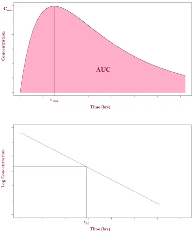
In Pharmacokinetic (PK) studies, inference is made on the absorption, dis-tribution, metabolism and excretion (ADME) of an externally administered com-pound within the body. This is done by measuring the concentration of the compound in some form of bodily tissue (such as whole blood or plasma) at a number of time points after administration. There are two approaches to PK analysis, modelling and non-compartmental (NCA). The modelling approach uses assumptions of the behaviour of the compound in the body to fit models to the data in order to approximate the concentration versus time curve. Whereas in NCA, no such assumptions are made, and numerical methods are used to ap-proximate this curve. The PK behaviour is summarised by PK parameters that are derived from this approximation, such as the area under the curve (AU C), the maximum concentration (Cmax) and the time at which this maximum occurs (tmax).

Acknowledgements

My first acknowledgement is to Lancaster University, both the Mathemat-ics & StatistMathemat-ics Department and the STOR-i DTC. When I first came to Lancaster seven years ago, I never imagined that I would find a home here, with the oppor-tunities that I have been offered. The enjoyment I found in my undergraduate studies motivated me to follow this path to a PhD, and the advantages (includ-ing fund(includ-ing) that STOR-i have given me have been indispensable. I have been lucky enough to have an amazing supervisory team during this PhD, both at the University and at Janssen. I’d like to thank Jack, Helena and Tom for all of their help, it has been a real pleasure working with them.

I would also like to acknowledge the friends that have shared the PhD ex-perience with me. Doing a PhD is not an easy three years, but supporting each other has been so important in both our successes and setbacks. Katie and Lucy have been blessings, and I know for certain that my PhD experience has been brighter because they have been a part of it.

I thank Emma, my best friend of many years, for the continuing under-standing, joy and laughter that a true friendship can bring. Weekends together have many a time been the calm in the storm and have given me the perspective so often needed in research, which has been a lifesaver in the PhD.

My fianc´e Matt, with whom I can’t wait to spend the rest of my life, never fails to surprise me in the ways in which he makes me smile. We have grown so much over the past seven years; even though the past three have been stressful for us both, we make the perfect team and have supported each other to make us shine both individually and as a pair. I’m so lucky to have found someone so amazing, and his love has been instrumental to get me where I find myself today. For this I am truly grateful.

have been a constant source of support in every way. Their ongoing faith has made me continue to work hard and I thank them unreservedly for this. I’m so appreciative of their loving help and guidance; I can only hope that my achieve-ments, including this PhD, make them proud of the daughter that they have inspired me to be.

My sister Lou, is the Anna to my Elsa. Her love, support and most impor-tantly belief in me has been integral not only in the past three years, but also the twenty-two before that. She has always helped me through the tough times and celebrated with me through the good times. I can never thank her enough for what she has done for me, but I hope that she realises how much she means to me and how much her help has contributed to the completion of this PhD.

Declaration

I declare that the work in this thesis has been done by myself and has not been submitted elsewhere for the award of any other degree.

Chapter 3 has been accepted for publication as Barnett, H.Y., Geys, H., Ja-cobs, T. and Jaki, T. (2017) Comparing sampling methods for pharmacokinetic studies using model averaged derived parameters.Statistics in Medicine.

Chapter 4 has been submitted for publication as Barnett, H.Y., Geys, H., Jacobs, T. and Jaki, T. (2017) Optimal Designs for Non-Compartmental Analysis of Pharmacokinetic Studies.Statistics in Biopharmaceutical Research.

The word count for this thesis is 42052 words.

Chapter

1 Background 1

1.1 Introduction . . . 2

1.2 Microsampling . . . 4

1.3 Pharmacokinetic (PK) Studies . . . 7

1.3.1 Modelling Approach . . . 10

1.3.2 Non-compartmental Analysis (NCA) . . . 17

1.3.3 Sparse Sampling Schemes . . . 18

1.4 Model Selection, Model Averaging and Simultaneous Inference for Multiple Parameters . . . 21

1.4.1 Model Selection . . . 21

1.4.2 Model Averaging . . . 22

1.4.3 Simultaneous Inference for Multiple Parameters . . . 23

1.5 Optimal Design Theory . . . 29

1.5.1 Model Based Optimality . . . 30

1.5.2 Cost-based Designs . . . 34

1.5.3 Application to PK/PD Studies . . . 34

1.5.4 D-Optimality for multiple response non-linear mixed ef-fect models . . . 41

1.6 Measurements that Cannot be Reliably Detected . . . 46

1.6.1 Definitions . . . 46

1.6.2 Methods . . . 48

2 Thesis Summary 51 3 Paper A: Comparing sampling methods for pharmacokinetic studies us-ing model averaged derived parameters 55 3.1 Introduction . . . 56

3.2.1 Baseline Method . . . 57

3.2.2 Extension . . . 63

3.3 Equivalence Testing . . . 65

3.3.1 Example revisited . . . 67

3.3.2 Simulation Studies . . . 68

3.3.3 Extension to Longitudinal Data . . . 73

3.4 Discussion . . . 75

4 Paper B: Optimal Designs for Non-Compartmental Analysis of Pharma-cokinetic Studies 78 4.1 Introduction . . . 79

4.2 Method . . . 83

4.3 Results . . . 86

4.3.1 Set Up . . . 86

4.3.2 Initial Results . . . 87

4.3.3 Comparison to Model Based Optimal Designs . . . 91

4.3.4 Application of Minimax Criterion . . . 93

4.4 Choice of Time Points . . . 95

4.5 Discussion . . . 103

5 Paper C: Methods for Non-Compartmental Pharmacokinetic Analysis with Observations below the Limit of Quantification 105 5.1 Introduction . . . 106

5.2 Methods . . . 108

5.2.1 Method 1: Replace BLOQ values with0 . . . 110

5.2.6 Method 6: Full Likelihood . . . 115

5.2.7 Method 7: Kernel Density Imputation . . . 116

5.2.8 Example Application . . . 118

5.3 Results . . . 119

5.4 Discussion . . . 127

6 Thesis Conclusions, Limitations and Further Work 130 6.1 Overview . . . 131

6.2 Conclusions . . . 131

6.3 Limitations . . . 133

6.4 Further Work . . . 134

Bibliography

137

A.2 For Candidate Model 3.2 . . . 144

A.3 For Candidate Models 3.6 and 3.7 . . . 144

B Sampling Time Points for Simulations 145

C Derivation of Second Order Approximation 147

D Average Bias of Parameter Estimates 150

E Additional TypeIError Rate Results 152

F Minimax Scenarios 154

Table

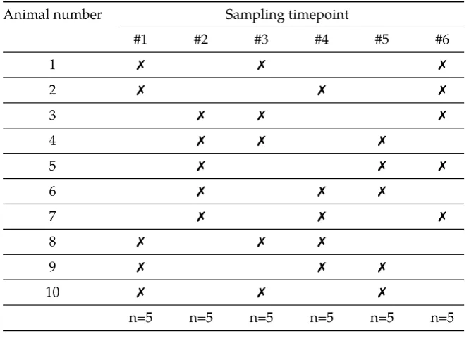
4.1 Sparse Sampling Scheme as suggested by Chapman et al.16 All main study animals are sampled, with 10 animals per sex per group. A total of 30 samples per sex per group are taken, with 3 per each of the 10 animals and 5 per each of the 6 timepoints. . . 81 4.2 The top 10 and bottom 10 ranking designs according to the

mini-mization of variance of the AUC estimate . . . 88 4.3 The top 10 ranking designs according to the minimization of

vari-ance ofΨ =w1var

d

AU C ∗

+w2var

d

Cmax

∗

withw1 =w2 = 0.5. Efficiency Measure for a given scheme is the ratio between the variance for that scheme and the best scheme, the larger the value, the less efficient the scheme. . . 92 4.4 Top 10 rankings of sparse schemes with choice of time points . . . 97 4.5 Top 10 rankings of sparse schemes with choice of time points by

Ψ =w1var

d

AU C ∗

+w2var

d

Cmax

∗

withw1 =w2 = 0.5. . . 97

4.6 Optimal Sparse Sampling Scheme with sampling time points (0.5, 1.0, 3.5, 4.0, 7.5, 12.0). 7 indicates that the individual subject scheme is shared by the scheme from Chapman et al16 and ◦ in-dicates that it is not. . . 102

5.1 The application of the seven methods to the motivating example illustrated in Figure 5.1. . . 119

B.1 Sampling Time Points Used in Simulation Studies . . . 146

D.1 The average bias of the estimate of the PK parameters. The true values aret1

E.1 Type I error rate for varying numbers of time points and combina-tions of PK parameters for an oral administration of a compound. Error bounds for 10,000 simulations are 2.214 and 2.806 for equiv-alence testing. . . 153 E.2 Type I error rate for varying numbers of time points and

combina-tions of PK parameters for an oral administration of a compound. Error bounds for 10,000 simulations are 2.214 and 2.806 for equiv-alence testing. . . 153

G.1 Top 5 overall schemes using time points(0.5,1.0,2.0,4.0,9.0,12.0) according to minimax criteria applied to equally weighted scaled sum ofAU C and Cmax variance: Ranks in the 8 scenarios, max-imum rank, and total sum rank. (* indicates the maxmax-imum rank for that scheme) . . . 157 G.2 Top 5 overall schemes using time points(0.5,1.0,2.0,4.0,9.0,12.0)

according to minimax criteria applied to equally weighted scaled sum ofAU CandCmax variance: Efficiency measure in the 8

sce-narios, maximum efficiency measure, and total sum efficiency mea-sure. (* indicates the maximum efficiency measure for that scheme)157 G.3 Optimal Time Point Choices Top 5 overall time point choices

ac-cording to minimax criteria: Ranks in the 8 scenarios, maximum rank, and total sum rank. (* indicates the maximum rank for that time point choice) . . . 158 G.4 Top 5 overall schemes using optimal time points(0.5,1.0,3.5,4.0,

7.5,12.0)according to minimax criteria applied to equally weighted scaled sum ofAU C andCmaxvariance: Ranks in the 8 scenarios,

H.1 Results showing average deviation from the non-compartmental

d

AU C _{and its variance with data generated from the fixed effects} model with higher dose and clearance. Results over 1000 simula-tions. (10 subjects, 6 timepoints) (A) = Analysed using arithmetic means. (G) = Analysed using geometric means. (N) = Confidence interval calculated using normal distribution on theAU Cd _{. (L) =}

Confidence interval calculated using log-normal distribution on theAU Cd _{. M1: Replace BLOQ values with 0, M2: Replace BLOQ}

values with LOQ/2, M3: ROS Imputation, M4: ML per timepoint Means, M5: ML per timepoint Imputation, M7: Kernel Density Imputation. * indicates not all analyses were successful. . . 160 H.2 Results showing average deviation from the non-compartmental

d

AU C_{and its variance with data generated from the mixed effects} model with higher dose and clearance. Results over 1000 simula-tions. (10 subjects, 6 timepoints) (A) = Analysed using arithmetic means. (G) = Analysed using geometric means. (N) = Confidence interval calculated using normal distribution on theAU Cd . (L) =

Confidence interval calculated using log-normal distribution on theAU Cd . M1: Replace BLOQ values with 0, M2: Replace BLOQ

H.3 Results showing average deviation from the non-compartmental

d

AU C _{and its variance with data generated from the fixed effects} model with lower dose and clearance. Results over 1000 simula-tions. (10 subjects, 6 timepoints) (A) = Analysed using arithmetic means. (G) = Analysed using geometric means. (N) = Confidence interval calculated using normal distribution on theAU Cd _{. (L) =}

Confidence interval calculated using log-normal distribution on theAU Cd _{. M1: Replace BLOQ values with 0, M2: Replace BLOQ}

values with LOQ/2, M3: ROS Imputation, M4: ML per timepoint Means, M5: ML per timepoint Imputation, M7: Kernel Density Imputation. * indicates not all analyses were successful. . . 162 H.4 Results showing average deviation from the non-compartmental

d

AU C_{and its variance with data generated from the mixed effects} model with lower dose and clearance. Results over 1000 simula-tions. (10 subjects, 6 timepoints) ((A) = Analysed using arithmetic means. (G) = Analysed using geometric means. (N) = Confidence interval calculated using normal distribution on theAU Cd . (L) =

Confidence interval calculated using log-normal distribution on theAU Cd . M1: Replace BLOQ values with 0, M2: Replace BLOQ

Figure

1.1 An illustration of some common PK parameters . . . 9 1.2 Diagram of intravenous bolus administration, one

compartmen-tal model . . . 11 1.3 Illustration of intravenous bolus administration, one

compartmen-tal model on a semi-logarithmic scale . . . 12 1.4 Diagram of intravenous bolus administration, two

compartmen-tal model . . . 12 1.5 Illustration of intravenous bolus administration, two

compartmen-tal model on a semi-logarithmic scale . . . 13 1.6 Diagram of oral administration, one compartmental model . . . . 14 1.7 Illustration of oral administration, one compartmental model on

a semi-logarithmic scale . . . 14 1.8 Diagram of oral administration, two compartmental model . . . . 15 1.9 Illustration of oral administration, two compartmental model on

a semi-logarithmic scale . . . 15 1.10 Illustration of linear interpolation between responses used in NCA. 18 1.11 Examples of different types of sparse sampling scheme . . . 19 1.12 Two different sampling grids: Uniform with respect to response

(left) and uniform with respect toAU C (right).26 . . . 37 1.13 MSE as a function ofN andkforu= 2.4,σ= 9and25≤N ≤4026 40 1.14 An illustration of the relationship between LOB, LOD, and LOQ,

3.1 Example dataset with individual concentrations (left) and spaghetti plot (right). . . 57 3.2 Comparison of observed typeI error rate for varying number of

time points and subjects for use of z and t quantile. Horizontal dotted lines show error bounds for 10,000 simulations . . . 63 3.3 Comparison of observed typeI error for varying number of time

points and subjects for use of 1st and 2nd order approximation. Horizontal dotted lines show error bounds for 10,000 simulations. 65 3.4 Comparison of observed typeI error for varying number of time

points and subjects for equivalence testing. Horizontal dotted lines show error bounds for 10,000 simulations. . . 69 3.5 Power of procedure for equivalence testing with 5, 20 and 100

sub-jects at 3 time points. . . 70 3.6 Power of procedure for equivalence testing with 5, 20 and 100

sub-jects at 7 time points for an oral administration of a compound. . 72 3.7 Type I error rate for varying numbers of time points for 5, 10 and

100 total subjects considering AU C and Cmax as PK parameters

for an oral administration of a compound. Horizontal dotted lines show error bounds for 1000 simulations. (Equivalence testing) . . 74 3.8 Power of procedure for equivalence testing for 5 time points for 5

and 10 total subjects consideringAU CandCmaxas PK parameters

for an oral administration of a compound. . . 75

4.1 An illustration of the population PK model described and the sampling time points. . . 88 4.2 The relationship between ranks given to schemes using MSE vs

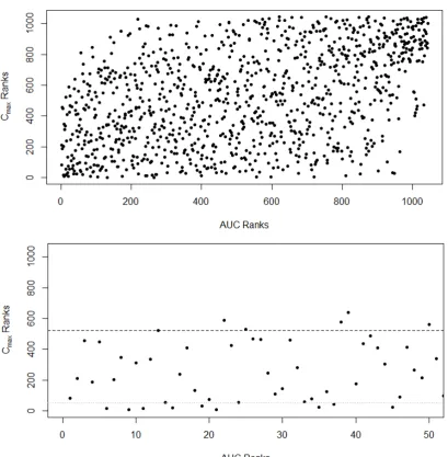
4.3 The relationship between ranks given to all schemes using the variances ofAU Cd andCdmax(top). The relationship between ranks given to schemes using the variances ofAU Cd andCdmaxfor the top 50 schemes according to theAU C ranks. Horizontal dashed line represents the top half of the ranks, dotted line represents rank 50 (bottom). . . 91 4.4 The relationship between ranks given to schemes using the weighted

sum of scaled variances ofAU Cd _andCd_{max, and}D_{-optimality. . . . 93}

4.5 Top 5 overall schemes according to minimax criterion applied to equally weighted scaled sum. Ranks for each of the eight scenar-ios are plotted. . . 94 4.6 Measuring the difference between the true population curve and

the simulated data at chosen time points. . . 99 4.7 Optimal Sampling Time Points . . . 100 4.8 Top 5 overall schemes according to minimax criterion applied to

equally weighted scaled sum for optimal time points. Ranks for each of the eight scenarios are plotted. . . 102

5.1 A motivating example, the red numbers indicate the number of observations that are BLOQ for that time point. . . 107 5.2 Regression on Order Statistics example illustrates how imputed

values are calculated. . . 113 5.3 A graphical illustration of the KD algorithm. Blue crosses indicate

a newkicalculated based on the currentfˆi. Green crosses indicate

previouski values. The red line indicates the LOQ. . . 117

5.5 Illustration of Example extended from Beal,10with smaller clear-ance and dose. The red numbers indicate the number of observa-tions that are BLOQ for that time point. . . 121 5.6 Results showing deviation from the non-compartmentalAU Cd _and

its variance with data generated from models with higher dose and clearance. Results over 1000 simulations. (10 subjects, 6 time-points) (F)=Data generated using fixed effects model. (M)=Data generated using mixed effects model. (A)=Analysed using arith-metic means. (G)=Analysed using geometric means. M1: Replace BLOQ values with 0, M2: Replace BLOQ values with LOQ/2, M3: ROS Imputation, M4: ML per timepoint Means, M5: ML per time-point Imputation, M7: Kernel Density Imputation. . . 123 5.7 Results showing deviation from the non-compartmentalAU Cd and

5.8 Results showing deviation from the non-compartmentalAU Cd and

Background

In order to ensure the protection of human subjects in clinical trials and future human patients, it is necessary to use laboratory animals in pre-clinical research. However, a balance must be established between the desire to cure disease in humans and the ethical considerations of the use of animals to achieve this.

These ethical considerations of using animals in drug development are en-capsulated by the 3 R principles: replacement, reduction and refinement.65 Re-placement involves finding different means of collecting the data that does not include the use of conscious living vertebrates. One option is absolute ment, where no animals are used at all. The other option is relative replace-ment, where animals that are not conscious living vertebrates are used. Relative replacement can be performed using, for example, in vitro methodologies or invertebrates such as nematode worms or fruit flies.

The second R of reduction is quite straightforwardly reducing the number of animals that are needed to take part in the study in order to still obtain the same quality and validity of results. Alternatively, by using the same number of animals to obtain additional information, one can reduce the number of future animals needed for such studies. This can be achieved by developing new exper-imental design and statistical analysis, in addition to better sharing of resources and data.

en-richment of the animals’ living environments in order to provide best for both their physical and behavioural needs.

A fourth R, responsibility,8is also considered by some. This is the respon-sibility of those working with animals in pre-clinical research. The nature of this slightly overlaps with the third R of refinement, as the responsibility of the re-searchers to treat the laboratory animals with respect and to care for the welfare of the animals is partly encompassed by the criteria of refinement.

One of the most recent developments in laboratory techniques to improve the outlook for laboratory animals is the novel blood sampling method of mi-crosampling (discussed in Section 1.2). This new sampling technique, which requires a reduced volume per sample, is the main motivation behind this re-search, covering considerations in the issues of reduction and refinement, and of course responsibility. The area of application of this technique that we focus on in this research is for pharmacokinetic (PK) studies in pre-clinical research (discussed in Section 1.3).

Microsampling is an important step forward for pre-clinical research, hence for it to be more widely used, there must be clear evidence that it gives equiv-alent results to previous sampling methods used, the subject of the first paper in this thesis (Chapter 3). It must also be ensured that the PK studies collect the most accurate information they can, this is done by controlling the sampling times to construct an optimal design, the subject of the second paper in this the-sis (Chapter 4). The subject of the third paper is considering how to deal with concentration values that are too low to be reliably detected in such PK studies (Chapter 5).

1.2

Microsampling

tens of thousands of euros.24 The blood : plasma ratio and whether the hemat-ocrit, blood cell partitioning and unbound fraction in plasma are constant were all found to affect the appropriateness of the use of DBS.

CMS uses a predefined low volume of sample collected in a glass capillary micropipette from, for example, the tail vein of a rat. This volume ranges from

8_-25_{µL for whole blood and}32_or64_{µL for plasma collection.}21

The process in-volves filling the glass capillary end to end with capillary force, then placing the capillary in a sample tube before washing out the sample by mixing with water or internal standard (IS) solution and leaving the capillary in the tube.48 This diluted sample can then be handled in the same way, with the same laboratory apparatus, as standard plasma samples are dealt with currently. The appropri-ateness of CMS is more vast than DBS and hence its potential usefulness is more widespread, so it may be used in a wider range of studies than DBS. This is be-cause it offers handling of samples of blood, plasma and other biofluids in the liquid state.56

In May 2013 the NC3Rs held a workshop in central London titled ’Over-coming the barriers for uptake of microsampling techniques in regulatory toxi-cology’. This comprised of representatives from pharmaceutical companies and regulatory bodies to share knowledge and information on microsampling and what the barriers were for further implementation. It was found that there were two main aspects contributing to the barrier: (i) functional and clinical pathol-ogy evaluation and (ii) approaches to bioanalysis and toxicokinetics (TK). This illustrates the reluctance of companies to embrace the use of microsampling, and suggests further evidence is needed to support its usage.

warmed prior to sampling to increase the blood flow, as they did for traditional methods.48 As well as this, the time that the animals have to be restrained is re-duced. This all reduces the stress that the animals are under and hence aids the refinement of the study procedure. The use of capillary microsampling makes use of current laboratory apparatus and procedure for analysis and hence only the sampling procedure changes which reduces retraining needed.

However, one of the main potential benefits of microsampling is the pos-sible reduction of number of animals needed in such studies. Currently, two separate groups of animals are often needed for pre-clinical and toxicokinetic studies, the main study animals in which the pharmacodynamics (therapeutic or adverse effects) are measured, and the satellite animals in which the pharma-cokinetic (PK) or toxipharma-cokinetic effects are measured. This is because the large blood volume of the sample taken for PK or TK analysis can cause anemia or other secondary effects such as bone marrow or haematological changes that could potentially confound the interpretation of the primary endpoints of the study.16 For example, in a typical repeated oral dose 4 week rat study with 10 study animals per dose group of each sex, an additional 3 to 9 satellite animals per sex are required.

toxicologi-cal endpoints in a regulatory repeated dose toxicity study of at least two weeks length.58 These results suggest that the use of microsampling may facilitate the elimination of the use of satellite animals.

Microsampling has already started to be implemented by some compa-nies in the drug development process. Anecdotal evidence exists for its use in non good laboratory practice (non-GLP), it has not been widely practiced and extended to good laboratory practice (GLP), which must adhere to a strict set of principles regarding such factors as consistency and reproducibility.58 It is hoped that more research and development in the area of microsampling will provide evidence that will help extend its usage and contribute to reduction and refinement in pre-clinical studies.

1.3

Pharmacokinetic (PK) Studies

This section provides some background to the basic concepts of pharma-cokinetics. Since the contents of this section are largely well known and estab-lished concepts in pharmacokinetics, many of the individual ideas and formula-tions are not referenced. The background information is largely based on books by K ¨all´en,49 Gibaldi32and Jambhekar & Breen.45

Pharmacokinetics is the study of the movement of drugs over time through-out the body. That is, it is concerned with the effect the body has on the drug. This is split into four main categories:

• _{Absorption- how drugs move from the site of administration (oral,} in-halation, etc) to the blood. This does not apply to drugs given by intra-venous pathways, as the drug is directly administered to the blood in that case, and there is no need for it to be absorbed;

• _{Metabolism- how drugs are transformed or broken down by the body} into smaller molecules, which may or may not be pharmacologically ac-tive or toxic;

• _{Excretion- how drugs are removed from the body.}

These four aspects are often referred to as the ADME process.

Typically one can only measure the concentration of the drug in some com-partment such as whole blood serum or plasma, and do so at specific predefined time points. The aim of pharmacokinetic studies is to then derive as much in-formation as possible about how the body handles the drug from only these measurements.

Some common PK parameters of interest that are estimated from this are: • Cmax- the maximum plasma concentration of the drug;

• tmax- the time the maximum plasma concentration of the drug is reached;

• AU C_{- the area under the concentration versus time curve, a measure of} exposure to the drug;

• t1

2 - elimination half life, the time taken for the plasma concentration to fall to half its maximum value.

These are illustrated in Figure 1.1 with the bottom graph on a semi-logarithmic scale for the elimination phase. That is, using a linear scale on the x-axis and logarithmic scale on they-axis.

Figure 1.1: An illustration of some common PK parameters

1.3.1

Modelling Approach

In the modelling approach, the concentration of the drug in the blood plasma is described by a mathematical model. Often these models are derived from assumptions that involve a simplification of the body by breaking it down into compartments, and modelling the diffusion of the drug between these com-partments. The more compartments considered, the more complex the PK model.

The choice of model depends on the distribution characteristics of the drug following its administration. The general rule is that the slower the distribution of the drug in the body, the more compartments are required to characterize the concentration versus time curve. Therefore for drugs that are rapidly dis-tributed, a one-compartmental model will adequately describe the plasma con-centration over time.

The model is also dependent on the route of administration of the drug. Drugs can be administered in two main ways: oral administration and intra-venous (IV) administration. IV administration involves delivering the drug di-rectly into the bloodstream. This can be as an infusion, with a slow increase in concentration, or as a bolus dose, with a very rapid increase in concentration. Oral administration involves ingesting the drug through the digestive system, and hence the absorption of the drug into the bloodstream must be modelled.

When fitting a PK modelC(t)to datay(t), it is assumed that the data is re-lated to the PK model by an error modele(t), either additively (1.1) or multiplica-tively (1.2). Realizations from the error modele(t)are assumed to be normally distributed with 0 mean.

Additive Error Model:

y(t) = C(t) +e(t) (1.1)

Multiplicative Error Model:

What follows are four of the main PK models generally used (although many others are used in practice):

1.3.1.1 Intravenous bolus administration, one compartmental model

In this case the body is modelled as one compartment, with the bolus dose administered directly to this compartment. Therefore the model is solely de-scribed by the elimination of the drug from this compartment, as there is no absorption phase. Figure 1.2 shows a diagram of this system.

Figure 1.2: Diagram of intravenous bolus administration, one compartmental model

The differential equation used to describe the rate of change of plasma con-centration is given in equation 1.3. The integrated equation for this model is given in equation 1.4 whereC(t)is the plasma drug concentration at timet,C0

is the plasma concentration at time 0 andkeis the elimination rate constant.

dX1

dt =−ke·X1 (1.3)

C(t) =C0e−ket (1.4)

Figure 1.3: Illustration of intravenous bolus administration, one compartmental model on a semi-logarithmic scale

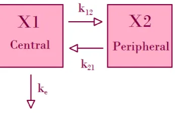
1.3.1.2 Intravenous bolus administration, two compartmental model

Here the body is modelled as two compartments, a central compartment (blood, liver, kidneys) and a peripheral compartment (fat, bone, skin). Again, the bolus dose is administered directly to the central compartment, so there is no absorption phase. However since there are two compartments, the rates of dif-fusion between the compartments must be taken into account. Figure 1.4 shows a diagram of these compartments.

Figure 1.4: Diagram of intravenous bolus administration, two compartmental model

com-partment. The integrated equation for this model is given by equation 1.6.

dX1

dt =−ke·X1−k12·X1 +k21·X2 (1.5)

C(t) =Ae−αt+Be−βt _(1.6)

Figure 1.5 shows a graphical illustration of such a model, with the two phases: distribution and post-distribution.

Figure 1.5: Illustration of intravenous bolus administration, two compartmental model on a semi-logarithmic scale

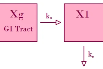
1.3.1.3 Oral administration, one compartmental model

When the drug is administered orally, the plasma concentration depends on the absorption from the gastro-intestinal (GI) tract to the compartment as well as the elimination from the compartment. Figure 1.6 shows a diagram of this process.

Figure 1.6: Diagram of oral administration, one compartmental model

scale.

dX1

dt =ka·Xg−ke·X1 (1.7)

C(t) = kaF D

V(ka−ke)

(e−ket−e−kat) _(1.8)

Figure 1.7: Illustration of oral administration, one compartmental model on a semi-logarithmic scale

1.3.1.4 Oral administration, two compartmental model

central, and the rate of elimination from the central compartment. Figure 1.9 shows a diagram of this flow between compartments.

Figure 1.8: Diagram of oral administration, two compartmental model

The differential equation to describe the rate of change of concentration in the central compartment is given in 1.9, with the integrated equation given in equation 1.10.

dX1

dt =ka·Xg+k21·X2−(k12+ke)·X1 (1.9)

C(t) = Ae−αt+Be−βt +Ce−kat _(1.10) Figure 1.9 shows the graphical representation of how the log plasma con-centration changes over time, with theαandβphases labelled.

1.3.1.5 Calculation of PK Parameters

Once the corresponding model has been fitted to the data and model pa-rameters calculated, the PK papa-rameters can be estimated as functions of these parameters. For example, for the one-compartmental oral dose model,tmaxcan

be calculated by differentiating the concentration versus time model with re-spect tot, setting equal to 0 and solving. This gives:

tmax =

logka−logke

ka−ke

.

The maximum concentration,Cmax, is then given by substituting int = tmax to

the model:

Cmax =

kaF D

V(ka−ke)

(e−ketmax−e−katmax).

TheAU CT (Area under the concentration versus time curve until time T) can be calculated by integrating the concentration versus time model overtbetween t= 0_andt=T_{, giving:}

AU CT =

kaF D

V(ka−ke)

exp(−kaT)−1

ka

−

exp(−keT)−1

ke

.

Then in the limit asT → ∞, we obtain: AU C∞= kaF D

V(ka−ke)

1 ka − 1 ke .

The variances of these estimates can be approximated using the variance-covariance matrix of the model parameters from the model fitting, and the delta method (covered in Chapter 3).

1.3.1.6 Non-Linear Mixed Effects Models

consider each subject in the population having their own individual model pa-rameters.

Take for example the volume of distribution parameter in the one compart-mental oral dose PK model. It may be assumed that the parameter has additive random effectsVi = ˜V +ηi or exponential random effectsVi = ˜V expηi, where

˜

V _{is the population parameter,}Vi is the individual parameter andηi ∼N(0, σ2)

for some varianceσ2. If more than one model parameter has mixed effects then there may also be a correlation between the random effects. In this framework, individual PK parameters can be estimated as well as population PK parameters.

1.3.2

Non-compartmental Analysis (NCA)

In this approach, no assumptions are made on the processes within the body that control the ADME process and hence no models are fitted to the data in the analysis. This offers the obvious advantage that with fewer assumptions, there is less room for error due to mis-specification of the model, and also avoids any complication that may arise in model fitting if the data is not harmonious with the model.

Since no model is fitted in the analysis, an approximation to the concentra-tions versus time curve must be made by some other means. The most preva-lent method uses a linear approximation between measurements, as illustrated in Figure 1.10.

The non-compartmental estimate to theAU Cfor an individual subject can then be calculated using the trapezium rule as follows:

[

AU C= J

X

j=1

ωjCj, (1.11)

Figure 1.10: Illustration of linear interpolation between responses used in NCA.

concentration at timetj andωj are weights defined as: ωj =

tj+1−tj−1

2 for j = 1,2, . . . ,(J−1), = tJ −tj−1

2 for j =J.

For a population estimate, one may instead use the mean concentration observed at each timetj.

1.3.3

Sparse Sampling Schemes

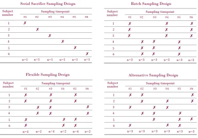
for subjects to be sampled at multiple timepoints but do not place the restriction on the timepoints that they must be split into disjoint batches. The designs are restricted however by the rule that for each set of timepoints that a subject is sampled at, at least two subjects must be sampled at these timepoints. This can result in unbalanced designs, i.e. different numbers of subjects sampled at each timepoint. The final type of sparse sampling design considered is the alternative sampling design. Here there is no restriction on when each subject can be sam-pled, although in the example in Figure 1.11 the number of subjects sampled at each timepoint has been restricted in order to make the design balanced.

Figure 1.11: Examples of different types of sparse sampling scheme

point6, 44, 55, 71 and for batch sampling designs.37, 41, 75 The basis of these methods is that the variance of the totalAU Ccan be estimated based on the sample vari-ance of the individual partial AU Cs for each batch. The variance of the AU C[ until the last observed timepointtJ is calculated by the following.

LettingJb ⊆ {1, . . . , J}be the indices of time points investigated in batch b= 1, . . . , B_,nbthe number of subjects in batchbandXitjthe observed response of subjectiat timetj. The approximation of the variance is given by:

b

V(AU C[) = B X b=1 s2 b nb , _(1.12) where

s2_b = 1

nb−1 nb

X

i=1

X

j∈Jb

ωjXitj− 1 nb nb X k=1 X

j∈Jb

ωjXktj

!2

.

Full sampling designs and serial sampling designs are special cases of the batch design. Full sampling considers one batch of subjects, with all timepoints investigated for that batch. Serial sampling considersJ batches, each batch with only one timepoint investigated.

For the flexible sampling designs, the method for approximating the vari-ance of the AU C[ is more complex.43 Again, the variance of the total AU C is estimated based on the sample variance of the individual partialAU Cs for each schedule. LetNjk be the number of subjects sampled at both time pointstj and tk,NJ the number of subjects sampled at timetj,Js ⊆ {1, . . . , J}be the indices of time points investigated in schedules,nsthe number of subjects on schedule s_, X¯j the mean of observed concentrations at time tj and δjs = Njns (that is the

proportion of samples at timetj that come from subjects on schedule s). The variance is then approximated as follows:

b

V(AU C[) = S X s=1 1 ns X

j∈Js

X

k∈Js

where

ˆ

σj,k = Njk

X

i=1

Xitj−X¯j

Xitk −X¯k

(Njk−1) +

1− Njk_Nj 1− Njk_N

k

.

For all such types of design, the R package PK42can be used to approximate the variance of theAU C estimate in the NCA framework.

For the alternative sampling design, there is no analytic form of the vari-ance of theAU C. This is due to no requirements for repeated schedules. How-ever in practice, these designs are used and hence must be considered.

1.4

Model Selection, Model Averaging and

Simulta-neous Inference for Multiple Parameters

This section provides background to the issues of model selection, model averaging, and simultaneous inference for multiple parameters, as these are rel-evant for the work completed in Chapter 3.

1.4.1

Model Selection

In statistical inferences, including PK studies, the process of model selec-tion is an important one. The aim of the model selecselec-tion process is to find the best model out of a set of proposed models. There are various established meth-ods to do such.

For nested models, one may construct pairwise comparisons of models us-ing the Likelihood Ratio Test. This involves, say for model A with likelihoodLA

and pA parameters nested inside model B with likelihoodLB and pB

However more versatile and easier to implement methods are often pre-ferred, which make use of an information criterion in the form of a penalized likelihood function:

I =−2 log(L) +q, _(1.14)

whereLis the likelihood andqis a penalty function. Akaike’s Information crite-rion (AIC) uses the penalty functionq= 2p, wherepis the number of parameters in the model,2 and Bayes information criterion (BIC) uses the penalty function q = 2plogn where n is the number of observations. AICc is also often used,

which has penalty function q = 2p+ 2_nk₋(k_k+1)₋₁. This gives more of a penalty for extra parameters than the AIC, and asn gets very large, approaches the value of the AIC. The model with the smallest value ofI is deemed to be the best ap-proximating model.

Using one of these criteria, it is often the case that once the best model is chosen, then all further inference is conditional on the chosen model being the truth, which of course may not be the case. This provides the motivation for the use of model averaging, discussed in the following sections.

1.4.2

Model Averaging

Model averaging deviates from choosing one best model, instead includ-ing the variability in the model selection process in the estimation of parameter uncertainty.12, 17 The main idea is to give weightswkto each modelMk that are

then incorporated into the value and variance of the estimator of the parame-ter of inparame-terest. These weights are scaled such thatPKk=1wk = 1. The parameter

common to all models,θ can then be estimated by:

ˆ

θ =X k

wkθˆk, (1.15)

This poses two obvious questions, the first being how to estimate the weights and the second how to incorporate them in the value and variance of the esti-mator.

To consider how to estimate the weightswk, suppose there areK models with information criterionIk = −2 log(Lk) + qk for modelk , Buckland et al.12 consider the ratio:

Liexp(−qi/2)

Ljexp(−qj/2)

= exp(−Ii/2) exp(−Ij/2)

, _(1.16)

to compare modeliwith model j. Ifqi = qj, i.e. the penalties are the same for

each model then this is simply the ratio of likelihoods, which is the Bayes Factor for comparing simple models. If the prior odds ratio is 1, then this represents the value of the posterior odds ratio. Therefore a sensible choice ofwk12is:

wk =

exp(Ik/2)

PK

i=1exp(−Ik/2)

, k= 1, . . . , K. (1.17)

This ensures that two models with the same value ofIare given the same weight. The method of bootstrapping23 can also be used to estimate the weights. Resampling with replacement gives the bootstrap resamples that are then used to calculate the weights. The weightwkis the proportion of times in the bootstrap resamples that model Mk is chosen to be the best approximating model. This bootstrap method has the feature that if two models have identical likelihoods, the method will always choose one model over the other, even if that choice is random. Then the sum of the weights of the two models is the same as the weight of one of the models would have been, were the other model to have been omitted.

1.4.3

Simultaneous Inference for Multiple Parameters

a topic that has been of much discussion, especially in the context of clinical tri-als where there are multiple endpoints. This is due to the complications caused by attempting to compute the simultaneous comparisons, especially in terms of controlling the type I error rate.3 Attempting to carry out each test as if it were the only one, at the same type I error rate, will lead to misleading results and in fact invalidate the hypothesis tests.

One method of carrying out the comparison is adjustingp-values for these simultaneous hypothesis tests, building on the basic and widely used Bonfer-roni adjustment. The adjustedp-value is defined as, for a particular hypothesis within the many being tested, ‘the smallest overall (i.e., “experimentwise”)

signif-icance level at which the particular hypothesis would be rejected’73 . Therefore this adjustedp-value may be directly compared to a given significance level α, the null hypothesis is rejected if the adjustedp-value is less than or equal toα.

The Bonferroni adjustment alters the significance level used for each test. Sayknull hypothesesH1,H2, . . . ,Hkare being tested at an experimentwise sig-nificance level of α. Then hypothesis Hi is tested individually at significance level αi such that

Pk

i=1αi = α. It is standard for each αi = α_k, although it is

possible for the allocations to be uneven. Therefore in terms ofp-values, if pi

is the unadjustedp-value for testingHi, then using the equal allocation of

indi-vidual significance levels as described above,Hi is rejected whenkpi ≤ α. The

Bonferroni adjustedp-value is thereforepBonf =kpi.

Holm38 suggests an improvement on this adjustment by proposing a se-quential procedure for rejecting the hypotheses, a more powerful adjustment called Holm’s procedure. Consider again the situation withk null hypotheses as above. This method still has the experimentwise error rate of α but is less conservative. The unadjustedp-values are ordered so thatp1 ≤ p2 ≤ . . . ≤ pk.

For each hypothesis test,pi is compared to _n−αi+1 as opposed to

α

n. The adjusted

sequential nature of the procedure. The hypothesis associated with the smallest p_{-value is tested first, followed by the next largest and so on. The procedure is} stopped when a non-significant result is found, and all other tests are consid-ered non-significant. That is, Hi is rejected if (n −i+ 1)pi ≤ α provided that

(n−j+ 1)pj ≤α ∀ j < i.

A similar approach to Holm’s procedure is Hochberg’s procedure,36which is essentially the reverse of Holm’s, in that the hypothesis associated with the largestp-value is tested first. The same level of significance_n−αi+1 is used for each

test of hypothesisHi, and testing continues until a significant result is obtained, then all further untested hypotheses are considered significant. Hi is therefore rejected if(n−j+ 1)pj ≤α ∀ j ≥i.

For all hypotheses in a set of hypotheses, Simes68introduced the following global test: RejectH0 = {H1, H2, . . . , Hn} if pi ≤ (iα_n)for at least onepi, where thepi are the ordered unadjusted p-values. It was proven by Simes that when the tests are independent, this global test has levelα. For dependent tests, Simes provided simulations to show that the test also has levelαapart from in excep-tional circumstances. Thep-value for this global Simes test is simply the smallest of the npi_i values, sinceH0 is rejected if any npi_i ≤ α. This test is used as part of

Hommel’s procedure.39, 40

Both Holm and Hommel’s test are based around the closed test procedure principle52 that is as follows. Suppose we have a collection of n hypotheses: H1, H2, . . . ,Hn. Let all possible combinations of subsets of these hypotheses be

defined asHI =

T

{Hi :i∈I}for allI ∈K, whereK is the set of all non-empty

subsets of{1, 2, . . . , n}. For each HI, let there exist a test based on statisticTI.

DefineJ ∈K andJ ⊇I, so that subsetI is included in subsetJ. For any given α, HI is rejected if everyHJ is rejected at level αby the correspondingTJ. The

probability of wrongly rejecting at least one hypothesis when testing all ofHI is

To carry out the procedure, one starts with the global testHI =

T

{Hi :i=

1, . . . , n}. Then if this test is rejected at level α then continue to test at level α each subset ofn−1hypotheses. This process continues until either a test is not rejected at the levelα, or eventually all tests, including those of subset size 1 are rejected. If the test statistic is from a Bonferroni test, then the resulting closed test procedure is Holm’s procedure. If the test statistic is from Sime’s test, then the closed test procedure is Hommel’s procedure. In terms of adjustedp-values, let pI be the unadjusted p-values for hypothesisHI and testTI. IfpJ ≤α ∀ HJ :

J ⊇ I then rejectHI. The adjusted p-value forHI is therefore the largest of the pJ’s. This of course unfortunately means conducting tests for each of the possible combinations of subsets, which isPni=1

n i

= 2n−1, which will obviously get very large very quickly. In some cases, however, shortcuts exist so that all of the tests need not be calculated.

These methods all stand alone for the simultaneous inference of multiple parameters, which provides a benchmark for future methods. However for the purpose of this research, this inference must also incorporate the model aver-aging discussed previously. Jensen & Ritz47discuss simultaneous inference for model averaging of derived parameters, specifically for the use of finding the de-rived parameters Bench Mark Dose (BMD) and the lower limit of the confidence interval for this (BMDL) in non-linear dose response modelling. This is a spe-cial kind of effective dose estimation in toxicology that includes additional prior information available. This procedure involves calculating simultaneous confi-dence intervals for the multiple comparison procedure; the adjusted quantiles for these intervals (corresponding to the theory of adjusting p-values discussed previously) are based on correlation estimates between the multiple parameter estimates.

are assumed to follow a semi-parametric model, for example :

Yi ∼ N(µi(τ0), σ2), (1.18)

for some known linear or non-linear mean functionµi that depends on an un-known parameter vectorτ0.

The model-averaged estimate used is similar to that considered by Buck-land et al.,12 that is the weighted average of parameter estimates. In this con-text, considerK candidate models that may or may not be mutually nested are parametrized by parameters(τ1, . . . ,τK) of dimensions (p1, . . . , pK). Then for modelk = 1, . . . , K, there areLderived parameters of interest : θ1, . . . , θL. These are differentiable functions of the model parameters, so thatθ1k = g1k(τk), . . . , θLk = gLk(τk). Therefore the model averaged estimate of the parameter θl (l = 1, . . . , L)is the weighted mean of the estimatesθˆl1, . . . ,θˆlK from allK models:

ˆ

θl,M A = K

X

k=1

wkθˆlk= K

X

k=1

wkglk(τˆk), (1.19)

where thewk’s are the model specific weights such thatPKk=1wk= 1. It is noted that for these methods, the specification of the particular weights is not required, although one may use the methods suggested by Buckland et al.12

The simultaneous inference is based on the methods of Pipper et al.,57and depends on thepk-dimensional asymptotic expansion of the maximum likeli-hood estimatorτˆkfor each of theKmodels :

n12(τˆ

k−τk) =n− 1 2

n

X

i=1

(I_k−1)Ψe_ki+o_P(1) (1.20)

=n−12

n

X

i=1

Ψki+oP(1), (1.21)

whereIk−1 is the inverse Fisher information matrix for modelk and Ψe_{ki is the}

The key idea exploited by Pipper et al.57 is that the asymptotic representa-tion is retained for stacked parameter estimates. That is, the followingPKk=1pK

-dimensional asymptotic expansion: n12(τˆ−τ) =n−

1 2

n

X

i=1

Ψi+oP(1), (1.22)

where τˆ = (τˆ1, . . . ,τˆK), τ = (τ1, . . . ,τK) and Ψi = Ψ1i, . . . ,ΨKi. Since the

standardized score vectors, theΨi’s, are independent and identically distributed random variables with mean zero and finite variance, application of the central limit theorem gives asymptotic normality, that is:

n12(τˆ−τ)→D _MVNK(0,Σ) _as n → ∞, _(1.23)

where the variance-covariance matrixΣis defined as the limit in probability of n−1Pn

i=1Ψ

T

i Ψi as a consequence of the law of large numbers. By substituting in parameter estimates, a consistent estimator of the variance-covariance matrix is obtained: Σˆ = n−1Pni=1Ψˆ

T

i Ψˆi. Hence one can obtain estimates of the correla-tions between the different parameter estimates from different model fits to the same data.

An asymptotic approximation for a single model-averaged estimate may be obtained by use of the delta method,70a method which uses a Taylor expansion to approximate a vector. This approximation is given by47to be:

n12(ˆθ_{l,M A} −θ₀) =wT

dglk

dτ

T

n12(τˆ−τ) +o_P(1), _(1.24)

wherew = (w1, . . . , wk)and dg_dτlk is theK×pmatrix _dd_τglk(τˆ1)T, . . . ,(τˆK)T

for l = 1, . . . , L_{. The variance of the model-averaged estimate,} θˆl,M A, may be ap-proximated using the previous asymptotic results to be:

var(ˆθl,M A)≈n−1

dglk dτ w T ˆ Σ dglk dτ

w, _(1.25)

The combined asymptotic representation of the vector of the L model-averaged estimates is then written by Jensen & Ritz47as:

n12(ˆθ_{lM A}−θ₀) = (I_L⊗w)· dg dτn

1

2( ˆτ −τ) +o_P(1), _(1.26)

whereIL is theL×Lidentity matrix and _ddg_τ is theKL×pmatrix obtained by stacking the matrices dg_dτ1k, . . . , dg_dLk_τ .

A simulation study was carried out by Jensen & Ritz47 alongside appli-cation to example datasets from the literature in order to explore the coverage properties of this asymptotic approach. Performance is compared to various other methods, for example those of Buckland et al,12Wu et al,74the unadjusted Bonferroni and methods using a single model. Results from these studies show that using a single model can result in confidence intervals too narrow, as they do not include model uncertainty. Other methods show conservative coverage, especially in cases with high correlations.

The method introduced by Jensen & Ritz is the focus to build on for the work in Chapter 3, bearing in mind the improvement it offers over the other methods previously discussed.

1.5

Optimal Design Theory

1.5.1

Model Based Optimality

When considering optimal designs from a PK modelling approach, there are different types of optimality criteria. These are all based on the assumed PK model. This requires some initial notation to be defined. Observations{yij}are assumed to satisfy:

yij =η(x,θ) +ij, i= 1,2, . . . , n; j = 1, . . . , ri; n

X

i=1

ri =N, (1.27)

whereη(x,θ)is the response function ofmunknown parametersθ = (θ1, . . . , θm)

and design variables x. Consider a linear model, η(x,θ) = θTf(xi) where

f(x) = [f1(x), f2(x), . . . , fm(x)]T is a vector of known “basis” functions. The ij are uncorrelated random variables with zero mean and constant variance.

The design of the experiment is denoted as the collection:

ξN =

  

 

x1, . . . ,xn p1, . . . , pn

  

 

={xi, pi}n1, where pi =ri/N. (1.28)

Thexiare the design points, theri are the number of samples taken at pointxi fori= 1, . . . , nandN is the total number of observations.

The information matrixM(ξN)of the design is given by the sum of infor-mation matrices corresponding to individual observations::

M(ξN) = n

X

i=1

riµ(xi), where µ(x) =σ−2f(x)fT(x), (1.29)

such that

M(ξN)θ=Y, (1.30)

where

Y =σ−2

n

X

i=1

riyif(xi). (1.31)

the information matrix:

Var[θ] =D(ξN,θ)≈M−1(ξN,θ). (1.32)

The equation:

(θ−θˆN)TM(ξN)(θ−θˆN) =R2, (1.33)

defines an ellipsoid of concentration, which generates confidence regions for normal linear models.59 Therefore the “larger” the matrixM(ξN)(equivalent to the “smaller” the matrixD(ξN)) is, the“smaller” the ellipsoid of concentration will be. Hence in order to optimize the precision of the estimatorθˆN, one wishes to “maximize” the matrixM(ξN)or equivalently “minimize” the matrixD(ξN). This relationship can be shown by considering the following argument. In the case of a single parameterθ, one can construct an estimatorθˆN which is approximately normal with meanθtand varianceVN. The ratio

ˆ

θN_√−θt

VN is

approx-imately standard normal and hence the approximate confidence interval with coverage probability1−αis:

CI1−α=

θ: |θ√−θN| VN

≤zα/2

, _(1.34)

withzα/2representing the100(1−α/2)percentile of the standard normal

distri-bution. So in the case of:

yi =θt+i, i ∼ N(0, σ2), (1.35)

withσ2 known, the sample meanθˆN =

PN

1=1

yi

N ∼ N(θt, σ2

N)has that:

CI1−α,norm =

θ : |θ−θN|

σ/√N ≤zα/2

. _(1.36)

Since the square of the standard normal random variable is equivalent to χ21,

z_α/2 ₂ =χ2_1,αwhereχ12,αis the100(1−α)percentile of theχ21 distribution. Hence:

(θ−θˆN)2

σ2_/N =N M(θ−θˆN) 2 _∼χ2

whereM = σ−2 is the Fisher information of the random variable yi. Therefore an equivalent confidence interval to that of (1.36) is:

CI1−α,χ2 = n

θ :N M(θ−θˆN)2 ≤χ21,α

o

. _(1.38)

Extending to the case of an m-dimensional parameter θ, the direct analog of (1.38) is:

CI1−α,χ2 = n

θ: (θ−θˆN)TM(ξN)(θ−θˆN)≤χ2m,α

o

, (1.39)

withχ2m,α representing the 100(1−α)percentile of the χ2 distribution withm

degrees of freedom. Thus the ellipsoid of concentration is defined by the bound-aries of this confidence region.

The general optimization problem is defined as finding the solution: ξ_N∗ ={x∗_i, p∗_i}n₁∗ =arg min

xi,pi,nΨ [M({xi, pi} n

1)], (1.40)

whereΨis a scalar known as the criterion of optimality . The possible solutions are any combinations ofn support points out of the available choices (xi ∈ X

) and the number of replications ri at xi such that Pni=1ri = N and n ≤ N.

Thus this is a discrete optimization problem with respect to the frequenciesri

or equivalently the weightspi =ri/N

The most popular types of optimality criteria are described by Fedorov & Leonov28as the following:

• D-optimality:

Ψ =|D|=|M|−1. (1.41)

Often called the generalized variance criterion, this D-criterion seems a reasonable measure of the “size” of the ellipsoid of concentration de-fined in (1.33 ) because|D|

1 2

is proportional to the volume of the ellip-soid:

Volume=V(m)Rm|D| 1 2 ,

where V(m) =

πm2

Γ(m₂ + 1), (1.42)

• E_-optimality:

Ψ =λ−_min1 [M] =λ_max[D], _(1.43) whereλmin[B]andλmax[B]are minimal and maximal eigenvalues of the

matrix B respectively. The length of the principal axis of the ellipsoid of concentration is2λ

1 2

max[D], hence minimization of thisE-criterion also

leads to the reduction of the linear “size” of the ellipsoid. • A- or linear optimality:

Ψ =tr[AD], (1.44)

where A is an m ×n non-negative definite matrix known as a utility matrix and tr[B]is the trace of the matrixB. For example ifA=m−1Im

whereImis them×midentity matrix, then theA-criterion is based on

the average variance of the parameter estimates:

Ψ =m−1_tr[D] =m−1_tr[M−1] =m−1

m

X

i=1

Var(ˆθi). (1.45)

D-optimality tends to be the most popular criterion used by theoretical and ap-plied researchers sinceD-optimal designs are invariant with respect to nonde-generate transformations of parameters, e.g. changes in the parameter scale. Also, they perform well according to other optimality criteria.27

In order to compare two designs, one can use their relativeD-efficiency:5

EffD(ξN,1, ξN,2) =

_|

M(ξN,1)|

|M(ξN,2)|

1/m

. _(1.46)

IfM is a diagonal matrix andD =M−1then |M|−1/m=

m

Y

i=1

mii

!−1/m

= m

Y

i=1

dii

!1/m

, (1.47)

1.5.2

Cost-based Designs

It is often the case that there is an associated cost with a given design. When the costs are different for the set of designs considered, this can be in-cluded in the following way.

The general optimization problem denoted in (1.40) may be viewed as an approximation to the following optimization problem:

ξ_N∗ =_argmin ξN

Ψ [NM(ξN)], (1.48)

subject to

n

X

i=1

ri =N ≤N∗, (1.49)

It is described by Fedorov & Leonov28that when measurements at a pointxare associated with some penalty or cost denoted as φ(x), the constraint of (1.49) may be replaced by:

Φ(ξN) = n

X

i=1

riφ(xi)≤Φ∗, (1.50)

whereΦ∗is the constraint on the total cost. Equivalently in the continuous set-ting of thepi’s:

NΦ(ξN)≤Φ∗, where Φ(ξN) = n

X

i=1

piφ(x1). (1.51)

This optimization problem, due to the monotonicity and homogeneity of criteria

Φ, can therefore be written as:

ξ∗ =argmin

ξ Φ

Φ∗

Φ(ξ)M(ξ)

=argmin

ξ Φ

M(ξ) Φ(ξ)

. (1.52)

1.5.3

Application to PK/PD Studies

The standard model, slightly adapting the previous notation introduced in (1.27), used for observations in PK sampling is

wherexij is thejth sampling time for subject i, ki is the total number of mea-surements for subjecti. γiis the vector of individual parameters for subjecti. N is the total number of subjects in the study. Theij are the measurement errors with zero mean.

In the model based approach to finding sampling sequences such as that described by Gagnon & Leonov,30 the key is to find a closed form expression or approximation to the information matrix for a single multidimensional pointxi, that is the(ki×1)vector of responses for subjecti. A design regionXmust be de-fined, and then the construction of optimal designs is relatively straightforward using for exampleD-optimality.

As an illustration, Gagnon & Leonov30use the design regionXformed by the combinations ofr sampling times from a sampling sequence of 16 choices, and the cost function given by:

φ(xk) =Cv+Csk, (1.54)

wherekis the number of samples taken (the length of the sampling sequence),Cs

is the cost of collecting/analysing a single sample andCv is the cost of enrolling a single subject. Gagnon & Leonov30show that whenCs >0then it is possible for the sequences with smaller samples to become optimal. It is also noted that optimal designs may comprise of a mixture of sequences with different numbers of samples. It is important to realise that although this cost function refers to monetary cost, that is not necessarily the definition of the cost function. The ‘cost’ may be in terms of time, or stress to the animals, or even a statistical concept such as bias that is wished to be penalized.

se-quence.

The simplest case is considered first, in which all subjects have the same sampling schedule. That is,xij ≡ xj andki ≡ k for alli = 1, . . . , N. Two types of empirical approaches are discussed by Fedorov & Leonov:26

• _{Type I: Method E1 For each subject, find the individual} tmax (Tb_{i) and}

Cmax(Cb_i) :

b

Ti =xj∗(i), _where j∗(i) =_argmax

j yij, Cbi =yi,j

∗_(i). _(1.55)

To findAU C[i, numerical methods are used, then averaged over all sub-jects in the study, either using arithmetic or geometric means to obtain populations estimatorsAU C[E1,Tb_E1andCb_{E1. (The subscript}E_{stands for}

empirical). It is noted that for largeN this method will produce reason-able estimators, however in the case of sparse sampling, the next method may be more appropriate.

• Type II: Method E2 At each time point, average the response over all patients:

b

ηj =ηbjN =

1

N

N

X

i=1

yij, j = 0,1, . . . , k, (1.56) and build estimators for the population curve{bηj}:

b

TE2 =xj∗, Cb_E2 = b

ηj∗, _where j∗ =_argmax

j bηj. (1.57)

Note that geometric means may also be used in place of these arithmetic means. Then numerical integration algorithms must be used to estimate AU C_:

[

AU CE2 =

k

X

j=1

Z xj

xj−1

g(x,aj)dx, (1.58)

where g is an interpolating function with parameters aj chosen such thatgpasses exactly throughηbj−1 andηbj. These are expected to provide

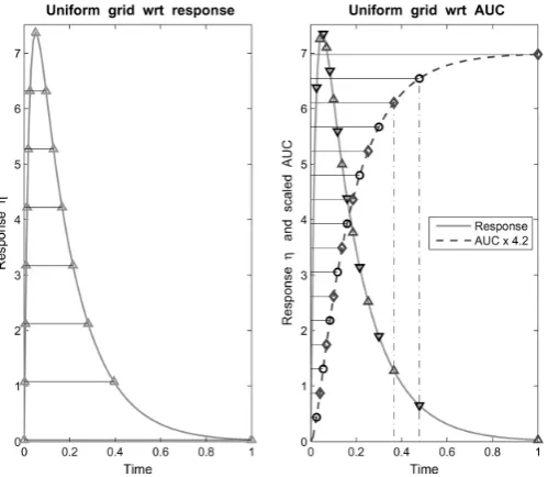
Figure 1.12: Two different sampling grids: Uniform with respect to response (left) and uniform with respect toAU C (right).26

The choice of sampling grid, that is the possible time points that samples can be taken, is often influenced by prior estimates of the plasma concentration curve. It is often the case that more samples are taken towards the start of the sampling interval and then the frequency of sampling decreases after the antici-patedtmax. Two types of sampling grid are proposed by Fedorov & Leonov,26as shown in Figure 1.12. The left hand panel shows a uniform grid on the vertical axis with respect to values of the response function, and then points are pro-jected onto the horizontal axis for sampling times. The right hand panel shows a uniform grid on the vertical axis with respect to the accumulatedAU Cvalue, and then points are projected onto the horizontal axis for sampling times.

Of course this requires preliminary knowledge of the plasma concentra-tion curve, but it is noted that so do tradiconcentra-tional sampling schemes. It is espe-cially common, as previously mentioned, to have a higher frequency of samples around the anticipatedtmax, which may be different for different trials.

ap-proximate the plasma concentration curve. This comparison is in terms of bias and variability of the three PK parameters previously discussed. The model based approach is found to perform best although the empirical approach also performs well.

A splitting of the sampling grid is also suggested, for example:

• _{Denote the single grid with}2k_{sampling points as}{xj :j = 1,2, . . . ,2k}.

• _{Collect samples for the first}N/2_{subjects at times}{x2j−1 :j = 1, . . . , k}. • _{Collect samples from the second half of the study cohort at} {x2j : j =

1, . . . , k}_.

• Using the method E2 for the estimation ofAU C2, average the responses

from each half of the cohort separately and then combine the series to obtain a population curve{ηbj}and estimate theAU Cusing (1.58).

Again, simulations are conducted and it is found that the split-grid approach results in a rather small loss of precision compared to the single grid approach. The mean squared error (MSE) of the estimate ofAU C for the single and split grids are compared using the empirical approach with the trapezium rule. In this case the response is approximated by the 2nd order polynomial with random intercept:

η(xj,γi) =γ0i+γ1xj +γ2x2j, (1.59)

where γi = (γ0i, γ1, γ2), E(γ0i) = γ0 and Var(γ0i) = u2. Let the M SE of the

ˆ

AU CE2 for the single grid beM SE1 and for the split grid beM SE2. LetBiasr

andV arrbe the corresponding bias and variance terms in the following expres-sion forM SEr:

M SEr=Bias2r+V arr, r= 1,2. (1.60) Assume a uniform grid{xj =jT /(2k), j= 0,1, . . .2k}and without loss of

if theij are assumed to have varianceσ2: Bias1 =

γ2

6 1

4k2, V ar1 =

1

N

σ2_(2k−0.5)

4k2 +u

2

∼ σ

2

2N k + u2

N, (1.61)

and for the split grid: Bias2 ≡Bias1, V ar2 =

(2k−1.5)2σ2

4k2_N +

u2

N

1− 1

2k2

∼ σ

2

N k + u2

N. (1.62) It follows from this that the measurement variability for the split grid is double that of the single grid, unsurprising since the number of samples taken is halved. However, the population component in the variance and the bias are the same for both grids. Hence when the population varianceu2dominates the measurement varianceσ2, then M SE1 ≈ M SE2, and this is in spite the number of samples being halved. However the single gird will always be better, and this difference depends on the values ofη00,σ2andu2. If costs are introduced however, this may not be the case.

Continue the notation introduced in (1.54) for costs, and let Ctotal be the

upper bound for the study budget. Then the overall costs are expressed as:

2kN Cs+N Cv ≤Ctotal for the single grid, (1.63)

kN Cs+N Cv ≤Ctotal for the split grid. (1.64)

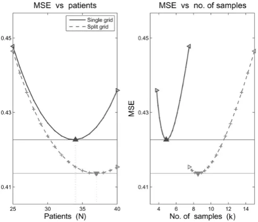
This may be approached by either selectingN and finding the maximal admis-siblek =k(N, Ctotal), or to selectkand find the maximalN =N(k, Ctotal). Note that the values ofkandN are not independent. A simulation study is conducted by Fedorov & Leonov,26 with the MSE of the estimate ofAU C from this study plotted in Figure 1.13, showing that the split grid may outperform the single grid in terms of this MSE.

Figure 1.13: MSE as a function ofN andkforu= 2.4,σ = 9and25≤N ≤4026