Composite particle algorithm for sustainable integrated dynamic ship
routing and scheduling optimization
Abstract
Ship routing and scheduling problem is considered to meet the demand for various products in multiple ports within the planning horizon. The ports have restricted operating time, so multiple time windows are taken into account. The problem addresses the operational measures such as speed optimisation and slow steaming for reducing carbon emission. A mixed integer non-linear programming (MINLP) model is presented and it includes the issues pertaining to multiple time horizons, sustainability aspects and varying demand and supply at various ports. The formulation incorporates several real time constraints addressing the multiple time window, varying supply and demand, carbon emission etc. that conceive a way to represent several complicating scenarios experienced in maritime transportation. Owing to the inherent complexity, such a problem is considered to be NP-Hard in nature and for solutions an effective meta-heuristics named Particle Swarm Optimization-Composite Particle (PSO-CP) is employed. Results obtained from PSO-CP are compared using PSO (Particle Swarm Optimization) and GA (Genetic Algorithm) to prove its superiority. Addition of sustainability constraints leads to a 4-10% variation in the total cost. Results suggest that the carbon emission, fuel cost and fuel consumption constraints can be comfortably added to the mathematical model for encapsulating the sustainability dimensions.
.
Keywords: Ship Routing, Carbon Emission, Mixed Integer Non-Linear Programming,
Maritime Transportation, Particle Swarm Optimization-Composite Particle.
1. Introduction
In maritime transportation domain, carbon emission is a topic of intense debate in the world shipping community. According to the United Nations Framework Convention on Climate Change UNFCCC (1997) Kyoto protocol, definite measures have to be taken in order to curb Carbon emission. Its main motive lies in restrainting the increase of the greenhouse gas emissions worldwide. Buhaug et al. (2009) stated that throughout the world, 4100 container carrying fleets operate, out of which only 4% are registered. Still 70 million metric tons (Mmt) of fuel was consumed in 2007 and 230 Mmt of CO2 emitted. This number shows that 22% of carbon emission and energy consumption are attributed to international shipping. According to International Chamber of Shipping (ICS), 25% of the greenhouse gas emissions in maritime industry are contributed by short sea shipping (ICS 2009). Now, this percentage may rapidly increase if there is no counteractions taken in order to lower the emission rate (IMO 2009c). International Maritime Organization (IMO) is exploring the possible measures which may help to reduce carbon emission from the available vessels by 20%-50% (IMO 2009c).
*Manuscript
IMO has already developed two measures EEDI (Energy Efficiency Design Index) for new vessels and EEOI (Energy Efficiency Operational Indicator) for existing vessels (IMO 2009a, 2009b, 2009c). IMO suggested several other measures like vessel size enlargement, voyage speed reduction, etc. In general, greenhouse gas emissions can be lowered in three distinct ways. Technological measures mainly involve the usage of alternative fuels such as biofuels, using energy-saving engines, more efficient ship propulsions, ship scrubbers which generally trap exhaust emissions and several other technologies that aim to reduce power consumption etc. There are two popular policies exist to account for carbon trading viz emission trading and carbon levy schemes. IMO has been working extensively on the introduction of these policies in the context of maritime transportation. Operational measures include speed optimization by ideally slow steaming, optimal fleet, route planning and other transportation based measures. Now all these effective measures can be implemented while addressing an equally important issue that deals with the increase in shipping costs.
Shipping costs primarily includes transportation costs, fuel costs, operating costs, hiring cost etc. To capture the carbon emission and bring sustainability issue into shipping operations, there is a need to combine carbon smission and maritime costs. In operational context, vessel speed optimization is an ideal strategy to reduce emissions and fuel consumption for a sustainable environmental condition.
logical to employ slow steaming as a prime strategy. Ronen (1982) used this strategy and stated that emission is proportional to fuel consumption which in turn is a cubic function of vessel speed. This relationship holds good approximation after a certain speed limit.
There is an increasing interest to investigate the possible ways to reduce the time spent by the ship in port. This issue can be addressed by considering a time window concept at each port. Most of the ports have definite operational restrictions during certain period of the day. Hence, port operations should categorically be carried out during that pre-defined time window. Port operations primarily involve loading/unloading of the products. Generally speaking, operating time at a port comprises of setup time and loading/unloading time. Fixed loading/unloading time is considered for each product. Port operation begins with the start of the time window. However, a vessel has to wait if it arrives much before the start of the time window. There is a possibility that the ship may finish its operation after the ending of the time window. In such cases a penalty cost is imposed depending on the total time operated outside the time window. Such measures help in maintaining port discipline and enhance the port management facilities.
Most liner shipping started to adopt the slow steaming policy from 2010 onwards. This strategy is useful in minimizing the total amount of CO2 emitted for a current maritime logistics scenario with low freight rates and high fuel prices.
voyage speed is decreased by 20%, then carbon emission and fuel consumption can be reduced by 20% and 40% respectively.
while it is at sea. While operating on ports, it runs on Marine Diesel Oil (MDO). There is a need to develop an emission coefficient for predicting the amount of CO2 generated for both types of fuel. From IMO 2000 study, it is concluded that emission coefficients of 3.082 and 3.021 can be considered for MDO and HFO respectively. Buhaug et al. (2009) have used similar emission coefficient in their paper.
Keeping in mind the slow steaming relationship with fuel cost, it is obvious to consider an appropriate fuel price coefficient for calculating the fuel cost. Fuel prices keep fluctuating from time to time as being market dependent. It can be assumed constant for computational benefit and for this paper average price considered for MDO and HFO are 463.50 USD/ton and 586 USD/ton respectively (values are taken from Kontovas et al (2011)).
In recent past, shipping lines are focusing more on mitigating ship emissions and fuel consumption in the prescribed sailing period. Fuel cost has become one of the most influential part of the total cost associated with maritime transportation. Already discussed earlier that slow steaming policy is a widely adopted operational measure to address sustainability aspects. A shipping company aims to lower the emission even when the vessels are operating at the port. Another objective is reducing the ship waiting time at the port in order to improve the service level.
plan depends on the schedule of the vessels of the shipping lines. The expected ship arrival times and departure times are regulated on the basis of shipping schedule and it gets disturbed owing to port congestion as mentioned in Notteboom (2006). Hence, for keeping proper coordination between the shipping lines and ports, vessel speed optimization can be considered as an ideal operational measure.
The contribution in this paper includes development of a new mathematical model considering planning horizon whereas in other papers only ship routing, loading/unloading operation are taken into account. The model predominantly deals with varying supply and demand rate for different products at each ports. It successfully integrates ship routing, scheduling along with slow steaming, carbon emission and fuel consumption. Slow steaming policy is incorporated for capturing the intricacies associated with sustainability in ship routing and scheduling. It is identified as an essential strategy for addressing the issues related to carbon emission. Different types of fuel oils are considered to map the realistic scenario in ports. This study integrates decision pertaining to fleet routing, multiple time window horizon and carbon emission associated with each vessel. An effective and intelligent search algorithm named PSO-CP is put to use for optimizing the developed mathematical model.
obtained from different instances are mentioned. Section 7 comprises of the conclusions and future scope of the research.
2. Literature Review
In the context of maritime logistics, researchers are showing keen intent in resolving the intricacies of carbon emission while dealing with mathematically grounded models.
2.1. Scheduling and routing models and methods
Christiansen et. al (1999) examined a fleet of ships transporting a single product (ammonia) between several production and consumption facilities. Here, the product is produced and stored in inventory facilities and later transported using a fleet of ships to several ports. The problem aims to design routes and schedules for a fleet of vessels in order to minimize the total transportation costs without any interruption of operations at the ports. Inclusion of time window concept in the model appears to be a possible scope of improvement. In subsequent years several articles related to inventory and routing problems are reported. Ronen, (2002) dealt with a maritime inventory routing problem considering multiple products. Their formulation addressed the intricacies associated with port inventory management. The routing part is missing in their formulation and it may affect the real life application of the model. Al-khayyal et al. (2007) studied a maritime inventory routing problem for multiple products and presented a mathematical model accordingly. They considered different compartments in the ship for accommodating multiple types of products. Song et al. (2013) proposed a new time-space network formulation incorporating various practical features associated with maritime inventory routing problem. Korsvik et al. (2011) introduced a tramp ship scheduling and routing problem and presented a mathematical formulation for capturing different dynamics of shipping operations. They proposed a large neighbourhood search heuristic for solving their problem. Stalhane et al. (2012) resolved a maritime pickup and delivery problem considering time window and split load. The main objective is to design a route for each ship by maximizing the total revenue generated and simultaneously minimizing the transportation cost. A novel branch-price-and-cut method is introduced for solving the new mathematical path-flow model of the problem. Agra et. al (2013) addressed a short sea fuel oil routing problem for multiple products with the inclusion of time window concept.
2.2. Models with time windows
unanticipated delays, Agra et al. (2013) presented a model considering penalty cost. Such type of costs are mentioned on various other articles within the bounds of maritime transportation. Babu et al. (2015) studied ship scheduling problem to cope with the rise in demand in Indian ports. Their problem reduced the delay of ships at port terminals by considering the time window concept and thereby improving the service level. In the context of ship routing and scheduling, Fagerholt (2001) incorporated penalty cost and soft time window horizon in their model to improve the service level. This helped in obtaining more acceptable ship schedules and reduce a substantial part of the logistics costs. Here, an inconvenience cost similar to penalty cost was imposed for servicing customers outside the time window.
2.3. Carbon emission consideration
Despite the fact that a considerably large amount of studies on maritime transportation are already present, very few papers have been published on the association between carbon emissions and maritime logistics. Lack of proper attention by the researcher shows that very few articles are available considering carbon emission during ship operation. The existing literature mainly revolves around ship design, propulsion, combustion and impact of emissions on weather and climate. Corbett et al. (2003) examined the techniques of constructing fuel-based inventories based on ship emissions. Endresen et al. (2003) researched on emission from cargo and passenger ships in the context of international trade situation. Eyring et al. (2005) introduced an approximate estimate for the total fuel consumption and global emission from international shipping over the past five decades.
capturing the relationship between vessel speed and bunker fuel consumption rate. It aims to minimize bunker fuel costs considering the possible service route, service frequency and number of ships to be deployed. Yin et al. (2014) studied the application of speed reduction in liner shipping and presented a cost model in order to exemplify the effect of slow steaming on revenue change.
Most the work associated with ship routing and scheduling fail to apprehend the importance of time window horizon. The mathematical model developed here considers time window concept while taking into account the broad formlation. Ship routing and scheduling problem has been studied by several authors such as Stalhane et al. (2012), Agra et al. (2013), Song et al. (2013), Agra et al. (2014) etc. But their respective problems overlooked the effects of carbon emission, fuel consumption in the context of maritime transportation. Andersson et. al (2014) incorporated the slow steaming policy on a fleet deployment problem but overlooked the fuel consumption related aspects. Yao et al (2012) dealt with fuel consumption and ship speed but avoided the intricacies associated ship routing and scheduling. It is absolutely clear that all the earlier researches focussed primarily on either maritime transportation or just carbon emission and fuel consumption. In this paper, the ship routing and scheduling operations are addressed while trying to curtail the carbon emission. The model developed considers slow steaming policy as an operational measure for addressing the effects of carbon emission, fuel consumption etc. The problem attempts to bridge these gaps in the literature by developing an optimization approach considering a detailed approach within maritime transportation domain.
3. Problem Description
Inter-port distribution problem is considered for a certain planning horizon. The objective is to design routes and schedules for a fleet of ships among all the ports with an aim to meet the demand and supply of each product. The problem considers several time window constraints addressing the practicality of the port operations. This problem ensures proper utilisation of the capacities of ports, depots and ships. Slow steaming policy is incorporated in the model for optimizing the amount of carbon emission generated.
Considering the underline problem, we come to understand there is a stark similarity among the vehicle routing problems (VRP), pick-up and delivery problems (PDP), road distribution by trucks (Tasan et al (2012), Beheshti et al (2015), Kachitvichyanukul et al (2015)). All these problems and their different variations such as pickup and delivery problem with time window (PDPTW) and multi-vehicle pickup and delivery problem (m-PDPTW) are well proven NP-Hard problems as stated in several articles (Zare-Reisabadi et al (2015), Yu et al (2016), Avci et al (2016), Zachariadis et al (2015)). PDP, m-PDPTW type of problems are closely related to ship routing and scheduling problem, but there is a significant differences like tramp ship specific approaches.
Our problem is formulated as MINLP comprising of routing variables, time window variables, loading and unloading variables, velocity variables etc. The major complexity in resolving the ship routing problem is observed due to large number of variables and constraints and these details are presented in table 8. For each of the problem sizes mentioned in the table, the possible combinations of variables and constraints are growing exponentially. The difficulty in the solution of the ship routing problems is that most of them belong to the class of combinatorial optimization problems characterized as NP-Hard. Computational time needed to arrive at the solution for the aforementioned problem is exorbitantly high even for a moderate size problem. While solving the MINLP model through mathematical programming and exact heuristics methods deteriorates the computational efficiency (Repoussis et al (2010), MirHassani et al (2011)). As a result, the complex problem requires a random search or heuristic search approaches. Keeping in mind that complexity of our problem and the similarity with the aforementioned problems, it is advisable to treat it as a NP-Hard.
Such a complex problem requires effective and intelligent search heuristics. As a result, particle swarm optimization for composite particle (PSO-CP) is employed to optimize this problem.
The problem considered pertains to one of the major sections of the maritime transportation domain. Here, products are imported from a certain port and distributed to some other port depending upon its requirement. The main aim is to design a mathematical model in order to predict an optimal schedule for routing of a fleet of vessels between different ports. The model integrates vessel speed optimization into fleet deployment for addressing the sustainability aspects. The study interprets the impact of slow steaming on the reduction of carbon emission, fuel consumption and fuel cost. Two different types of engine fuel are considered over here. ne Diesel Oil while operating at port and Heavy Fuel Oil while sailing in the sea. Specifying different types of fuels helps in addressing the carbon emission aspects appropriately as it depends on the type of fuel consumed. The influence of carbon emission, fuel consumption and fuel cost on the total transportation cost is also depicted. Parameters such as speed ranges, product capacities and inventory restrictions at different ports are considered appropriately.
multiple products is to be met at different ports. Each port has a specific time window for conducting the port operations within the allotted time. A penalty cost is incurred if the time window is violated. A pictorial description of the time window horizon is mentioned in figure 1. Demand and supply of each product at each port is known beforehand. The initial inventory capacities are also assumed. Initial storage capacities of each product at each port are provided. Travel time of each ship from one port to another depends on the distance between two ports and velocity of the ship. The amount of product on board a ship at the start of the planning horizon is assumed beforehand. Carbon emission, fuel cost and fuel consumption related parameters are also considered.
<<Insert Figure 1>>
4. Mathematical Model:
This section presents the mathematical formulation for the aforementioned problem. The nature of demand and supply rates definitely have an impact on the underlying model. The problem is solved for a certain time horizon, definite number of ports, multiple types of product and precise number of ships. The time horizon considered in this problem is discretized to steps of equal periods/intervals (corresponding to days). Binary variables are considered for assessing the current status of each ship.
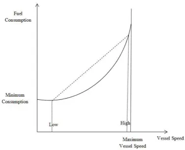
Fuel consumption is a non-linear function of sailing speed as mentioned in section 1. Ronen (1982) stated that, for speed values slightly more than certain minimum limit, fuel consumption per time unit can be considered as a convex cubic function of vessel speed. Figure 2 depicts the relationship between fuel consumption and vessel speed. The graph shows how fuel consumption is non-linearly dependent on vessel speed.
<<Insert Figure 2>>
A cubic function of vessel speed is embedded in the formulation for calculating the fuel consumption. Fuel consumption for the ship when it sails from one port to another is directly
proportional to speed.
Assumptions:
1. Considering the realistic scenario, a ship can initialize its operation in one period and can terminate its operation in the same time period or in the next time period.
2. Penalty cost is incurred if time window is violated. However, the ship may actually finish its operation during the next time window. To counter such situation, penalty cost is also imposed for the operation time in the next time window.
4. The overall model is developed keeping in mind that at most one ship can operate in a port at each time period.The uncertainties associated with multiple number of berths in each port is over-looked in the formulation.
Indices
p
Products,
q r
Portss
Shipss
q Initial port position of Ship
s
, l
k Time period
Sets
S Set of all the ships
R
Set of all the ports under considerationP
Set of productsK
Set of time periodsParameters
qr
L Representing the distance between port
q
and r Aqk
T Beginning of time window at port
q
in period k.B qk
T Ending of time window at port
q
in period kW qp
C Fixed cost associated with operation (loading/unloading) of product
p
at portq
qp
T Time required at port
q
for (un)loading one single unit of productp
qkp
D Demand at port
q
for productp
in time period kqrs
C Transportation cost for ship
s
once it travels from portq
to port rs
V Storage capacity for each ship
s
qp
Y Total storage capacity associated with the depot at port
q
for the productp
qp
U Set up time required for operating (loading/unloading) of product
p
at portq
sp
Q Amount of product
p
on-board a ships
at the starting of the planning horizonp qk
C Penalty cost per hour, associated with operation delay at port
q
in time periodkqp
J = 1, if port
q
is a supplier of productp
= -1, if port
q
has a demand of productp
= 0, if port
q
has no demand/supply of productp
s
B Maximum fuel consumption for ship
s
s
F Maximum fuel cost for ship
s
s
qs
f Fuel consumption at port
q
for ships
Continuous Variables
qk
t Starting time of operation at port
q
in period k, q R, k K Eqk
t Ending time of operation at port
q
in periodk , q R, k K. (E stands for ending of operation)qk
p Total operating time outside the time window at port
q
for periodk, q R,k K
qksp
Q Total quantity of product k loaded/unloaded at port
q
from ships
in period kq R k K, s S, p P. Qqksp 0if Jqp 0, or k 1, q qs
qksp
I Total amount of product
p
available on ships
while departing from portq
after anoperation that started in period k,q R,k K,s S ,p P.Iqksp 0, ifq qs
qkp
S Stock level at port
q
for productp
at the end of period k,q R,k K,p P
qrs
W Velocity of ship
s
while travelling from portq
to port r, For xqkrls= 0, and q = rqrs
W = 0. ,q r R, s S
Binary Variables
qkrls
x = 1, if ship
s
began its operation in period k at portq
and then travels from portq
to portrand initiate its operation at portrin periodl,= 0, otherwise, ,q r R, ,k l K,s S ,xqkrls 0if k l; or
q r
qks
z = 1, if ship
s
finally ends its route at portq
after an operation that started in periodk, = 0, otherwise, q R,k K,s Sqksp
O = 1, if product
p
is loaded/unloaded at portq
from ships
in periodk,= 0, otherwise; q R,k K,s S , p P. Oqksp 0, ifJqp 0; or k 1
The objective function
, ,
W P
qrs qkrls qp qksp qk qk
q r R k l K s S q R k K s S p P q R k K
Minimize C x C O C p (1)
Constraints
1, ,
rlqks r R l K s S
Equation (1) represents the objective function which aims to minimize the transportation cost, setup cost and penalty cost due to delay. Constraint (2) represents that in a given time period
k only one single ship s can operate in a given port q . This constraint guarantees that at a given time period at most one ship can operate in a certain port.
1 1 1,
s s
q rls q s
r R l K
x z s S (3)
1,
qksq R k K
z
s S
(4)0 , , >1,
rlqks qkrls qks
r R l K r R l K
x x z q R k K k s S (5)
Constraint (3) represents that either the ship s travels from its initial port q to port r or it ends its route at port q. Constraint (4) represent that ship s must end its route at some port q. Constraint (5) represents the flow conservation constraints for each period k and port q. This means that the ship must either sail from port q to port r or it might terminate its route in port
q, given that it started its operation in port q at period k.
,
A B
qk qk qk
T t T q R k K (6)
Constraint (6) represents the time window range.
( E qr ) 0, , , , ,
rl qk qkrls
qrs L
t t x q r R k l K s S
W (7a)
When xqkrls = 0,for a certain q, k, r, l and s,
( E qr ) = 0,
rl qk qkrls
qrs L
t t x
W (7b)
Constraint (7a) represents a scenario where a ship s (after completion of an operation in period k) is travelling from port
q
to port r (where a new operation will start in period l). Here, the port operation at port r will only start after the ending of operation at portq
plus the travelling time (which is distance travelled divided by the ship speed) from portq
to r.This constraint is considered only when the ship travels from port q to r.
q to r then naturally,
x
qkrls = 0. For such a scenario, we consider constraint (7b).0, ,
E
qk qk qp qksp qp qksp
s S p P s S p P
Constraint (8) represents the ending time of each operation on the basis of starting time of operation as well as set up time and total loading/unloading time for all the products.
0, ,
E B
qk qk qk
p t T q R k K (9)
Constraint (9) represent the operation time outside the time window.
, 1
0,
,
,
1
E qk q k
t
t
q R
k K k
(10)Constraint (10) depicts that for each port q and period k, the ship can start its operation once previous period operation is terminated.
0, , , ,
s qksp qksp
V O Q q R k K s S p P (11)
If a port operation takes place, then surely the amount of product p loaded/unloaded should be greater than zero. Constraint (11) addresses the above mentioned scenario.
( ) 0, , , , ,
qkrls qksp qp rlsp rlsp
x I J Q I q r R k l K s S (12)
Constraints (12) associates the product loaded/unloaded to the quantity on-board. This equation ensures that if a ship s travels from port q to r, then the quantity of product on-board while departing from port r should be equal to the quantity on-board while departing from port q plus/minus the quantity loaded/unloaded from port r.
0, , ,
s qkrls qksp
r R l k p P
V x I q R k K s S (13)
Equation (13) imposes an upper bound on the quantity carried by ship s. It represents a situation where ship must sail from one port to another only if the amount of product k on-board ship s is positive.
,( 1), 0, , ,
q k p qksp qkp qkp
s S
S Q D S q R k K p P (14)
Equation (14) aims to satisfy the demand for each product p at each port q in period k.
3
,
( E ) 0 , , ,
qr qrs s qk qk qs
q r R q R k K
e L W B t t f r R q r s S (15a)
Equation (15) ensures that fuel consumption for each ship s remains within the limit of maximum consumption. Here the velocity is considered as cubic function of fuel consumption.
3
Fuel consumption while the vessel sails from th port to port = th qrs
q r eW
( E ) 0
s qk qk qs q R k K
B t t f (15b)
0, , ,
qkp qp
S Y q R k K p P (16)
Equation (16) represents storage capacity constraint for each product p at each port q.
3
,
586 ( E ) 463.50 , , ,
qs qk qk s qr qrs
q R k K q r R
f t t F e L W r R q r s S (17)
When
x
qkrls = 0, constraint (17b) is used in place of constraint (17a).586 ( E )
qs qk qk s q R k K
f t t F (17b)
Constraint (17) imposes an upper limit on the total fuel cost incurred for each ship s. Average fuel prices are 463.50 USD/ton for Heavy Fuel Oil (Low-Sulphur Fuel Oil) and 586 USD/ton for Marine Diesel Oil (values related to different fuel oil prices are taken from Kontovas et al (2011)).
0, , , 1, ,
qksp rlqks
r R k K
O x q R k K k s S p P (18)
Equation (18) ensures that if ship s is operating at port q during time period k, then port q
must belong to the route of the ship.
3
,
3.021 3.082 ( E ) , , ,
s qr qs qk qk qs
q r R q R k K
E e L W t t f r R q r s S (19)
When
x
qkrls = 0, constraint (19b) is used in place of constraint (19a).3.082 ( E )
s qk qk qs
q R k K
E t t f (19b)
Constraint (19) ensures a check on carbon emission for each ship s. Emission coefficients for Marine Diesel Oil and Heavy Fuel Oil are 3.021 and 3.082 respectively (emission coefficient values are taken from Kontovas et al (2011)). This constraint restricts the carbon emission level within a certain allowable limit for maintaining a sustainable ship routing.
{0,1}, , , , , , , qkrls
x q r R q r k l K k l s S (20)
{0,1}, , , qks
z q R k K s S (21)
{0,1}, , , , qksp
O q R k K s S p P (22)
0, , , , qrs
0, , , qkp
S q r k K p P (24)
, 0, , , ,
qksp qksp
Q I q R k K s S p P (25)
, , E 0, ,
qk qk qk
t t p q R k K (26)
Equation (20), (21) and (22) represents the binary variables. Equation (23), (24), (25) and (26) represents the non-negativity constraints.
5. Solution Approach
MINLP model is developed for the problem described above. The nature of demand and supply rates might have an impact on the underlying model. The problem considered for a scenario having a precise time horizon, certain number of ports, multiple types of product and specific number of ships. The time horizon associated with the problem is discretized into steps of equal periods/intervals (corresponding to days). Binary variables are included for assessing the current status of each ship.
A variant of Particle Swarm Optimization of Composite Particle (PSO-CP) is employed for solving the MINLP model. PSO-CP was initially developed by Liu et. al (2010) in order to tackle dynamic environments. This concept was inspired from the phenomenon of interaction of elementary members in each composite particle through VAR (velocity-anisotropic reflection) scheme. It utilizes of a composite particle for considering valuable information sharing strategy in order to find better optima in the solution space. The enhance diversification of the composite particle helps integral movement while avoiding collision and velocity-slackening in the elementary particle. This algorithm incorporates the scattering operation policy for moving the fittest elementary particle to a better possible promising direction. The innovative and sterling qualities of the algorithm like construction of composite particles, scattering and VAR operation are adopted for designing a slight variant of PSO-CP for tackling the complex maritime transportation problem described earlier. Next sections 5.1, 5.2, 5.3, 5.4 and 5.5 presents the important operators associated with PSO-CP algorithm and section 5.6 provides an overview of the algorithm.
5.1. Composite Particle
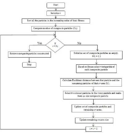
Composite particle is defined as a geometrical structure of three members having similar euclidean distance. It is constructed by
priority. Initially, all the particles are sorted in terms of their respective fitness values. Construction of composite particle is done by sorting out the particle with worst fitness value from the list. Then two other particles are selected from the list having minimum euclidean distance with the first particle. Henceforth, these three particles form the composite particle. Particles not belonging to the composite particles are
Numbers of independent particles depend upon the following formula, N1=swarm_size
function. For example, if swarm_size is a multiple of 3, suppose say 6, then N1 = 6
3*[(6-1)/3]. As largest integer function of [(6-1)/3] is 1, so N1 = 6 3*1 = 3. The construction of
composite particle is briefly depicted in figure 3 given below.
<<Insert Figure 3>>
5.2. Scattering Operation
Along with composite particle, scattering operation is also adopted because it promises to ameliorate the fittest elementary particle available to a more desirable direction. When the particles of the composite particle converge among themselves, the scattering operation is triggered. A kth composite particle converges only when the euclidean distance between the
worst particle (in terms of fitness) and next worst member of the composite particle is less than a threshold limit (Dk ). Suppose, let us consider the position of the elementary
particle having the best fitness value in the kth composite particle is represented by F. The
other two non-pioneer particles are denoted as A1 and A2. Then the particle with best fitness F
scatters along the direction in order to replace A1 and A2 using the repulsion mechanism
described as FS1 A F1 and FS2 A F2 . The parameter is a random vector generated between the acceptable scattering step range [Sstepmin,Sstepmax]. Now, the new composite particle comprising of F, S1 and S2 formed using scattering operation is shown in figure 4a.
pioneer k
x used in figure 5 represents the current position of the best fittest particle in kth
composite particle.
<<Insert Figure 4a>>
5.3. VAR (Velocity-Anisotropic Reflection) Operation
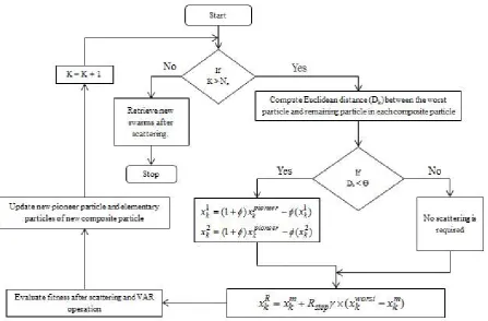
Now composite particle usually encounters two major concerns. The primary concern is to develop a method for increasing the interaction among elementary particles in order to explore promising search space. VAR scheme helps the elementary particles to look for more extensive solution space. VAR operation replaces the particle having the worst fitness value with an additional reflection point in the direction of more acceptable and fitter search space. Composite particles use this method to track more promising peaks in the new environment. VAR scheme also helps the pioneer particle in carrying out the valuable information sharing among other two elementary particles. Construction of composite particle using VAR operation is presented in figure 4b. The scattering and VAR operation are explicitly explained in the flowchart presented in figure 5. m
k
x mentioned in figure 5 represents the position of the
mth particle in the kth composite particle and worst k
x represents the position of the worst
particle in the kth composite particle. The R k
x denotes the position of the reflection point of
the mth particle ( m k
1, 2
k k
x x represents the positions of the two elementary particles in kth composite particle. Rstep
depicted in figure 5 denotes the reflection size parameter. is a random vector generated using uniform distribution.
<<Insert Figure 4b>>
<<Insert Figure 5>>
5.4. Swarm Representation
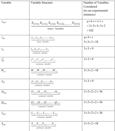
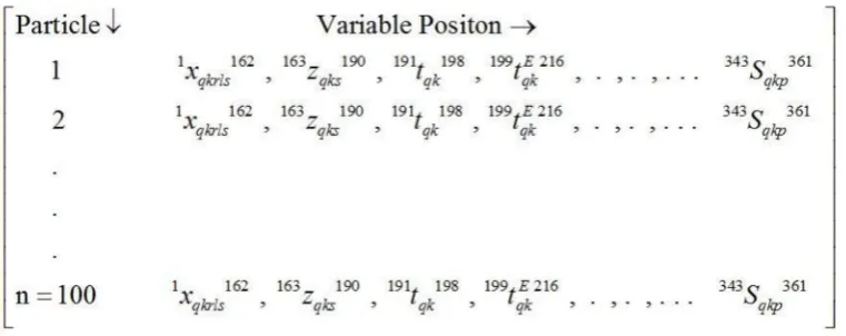
Each swarm is represented into sets of continuous time window variables (starting and ending time of operation), velocity variables (for individual ships between different ports), quantity variables (amount of product being loaded or unloaded), Stock variables (Stock level of different products at different ports), along with some binary variables for route scheduling and product allotment. For example, in case of a scenario with 3 ports, 3 time periods per planning horizon, 2 ships and 2 products, a schematic representation of the swarm is presented in table 1 and figure 6.
<<Insert Table 1>>
<<Insert Figure 6>>
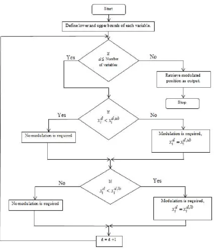
5.5. Position Modulation
Position modulation function ensures that all variables should lie within their corresponding boundaries. The function basically takes the swarm to be modulated as its input and modifies that swarm according to the predefined limits and gives the modified swarm as the output. The approach is briefly depicted with the help of the flowchart given in figure 7.
<<Insert Figure 7>>
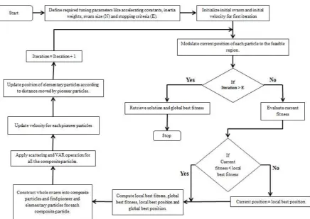
5.6. PSO-CP Algorithm Overview:
The algorithm begins with random initialization of the swarm and its initial velocity and runs in an iterative manner till the termination criterion is met. Each iteration involves tracking of the personal best for each pioneer particle, the global best particle, construction of composite particles, scattering operation, VAR scheme operation and updating the swarm for next iteration. The updating the velocity and position of a pioneer particle in a composite particle is done using the traditional PSO equations (27) and (28). Updation of the remaining two elementary particles takes place according to the distance and direction in which pioneer particle has moved.
1 2
( 1) : ( ) ( ( ) ( )) ( ( ) ( ))
i i i i g i
v t wv t c p t x t c p t x t (27)
( 1) : ( ) ( 1)
i i i
Where v ti( 1), ( )v ti is the velocity of ith particle for tth and (t+1)th iteration, x ti( 1), ( )x ti is the position of ith particle for tth and (t+1)th iteration, ( ), ( )
i g
p t p t are the local best position and global best position for the tth iteration, w is the inertia weight, c c1, 2 are the
acceleration coefficients and , are the random vectors.
At the end of each iteration the position of each updated particle is checked to ensure that it lies within its predefined boundaries using the position modulation function discussed above. When the termination criteria is reached, the algorithm attains a near optimal solution. Figure 8 presents the flowchart of the algorithm and different operations associated with it.
<<Insert Figure 8>>
6. Result and Discussion
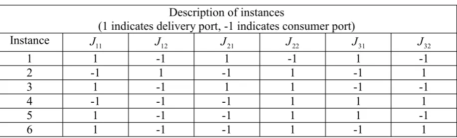
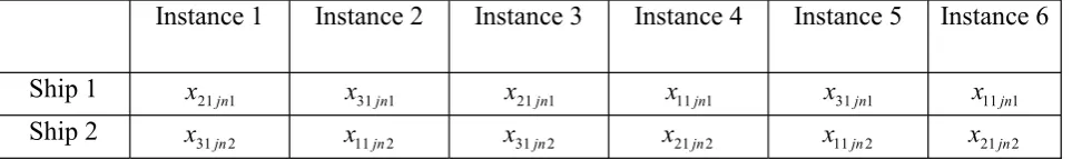
In this section, the results obtained by solving the proposed mathematical model are summarised. A small size numerical example is considered for performing the computational experiment in order to illustrate and substantiate the proposed model. The example considers 3 ports, 3 time periods for each planning horizon, 2 ships and 2 different types of products. Different instances are developed on the basis of demand or supply of each product at every port. Table 2 depicts the different instances considered. The data associated with operating costs, vessel capacity, time window information are appropriately generated using the data presented in different sources like Barnhart et. al (2007), Cullinane et. al (1999) and Chaug et. al (2005). The complete data considered for all the six test instances are presented in Table 3. For the given example, the initial ship position for all the six instances are presented in table 4.
<< Insert Table 2>>
<<Insert Table 3>>
<<Insert Table 4>>
All the experimental scenarios provided in Table 4 are solved using MATLAB R2014a installed in a machine having processor, 2.10 GHz CPU with 4GB RAM. Each instance is solved with algorithms PSO-CP, basic PSO and traditional GA. The performance of the algorithms are compared with each other. Parameter settings of the algorithms are carried out for obtaining the near-optimal solutions to the best possible extent. The crucial parameters involved in PSO-CP are accelerating coefficients, stretching parameters, diversification parameters, inertia weights and Euclidean distance limit. For obtaining the best parameter settings, 30 repeated test trails are performed corresponding to each parameter mentioned above. Values of stretching parameters and diversification parameters are directly adopted from the sensitivity analysis presented in Liu et. al (2010). Table 5 presents the desired value of each parameters associated with PSO-CP.
Every instance is run using algorithms PSO-CP, PSO and GA. The computation time is calculated for every instances. The final result obtained for the six different instances are given in the Table 6. This table presents the near-optimal solutions pertaining to each instance and corresponding computation time obtained through PSO-CP, PSO and GA. The results interprets that, there is a substantial difference in the values obtained using three algorithms. This enlightens the superiority of the PSO-CP agorithm when compared with PSO for the accuracy of the near optimal solutions. In terms of the computational time, performance of the PSO-CP can be considered as good as PSO and GA.
<<Insert Table 6>>
Similarly, to quantify the effect of sustainability related constraints on the total cost, the proposed model is optimized twice. Initially PSO-CP algorithm helps in solving the model considering the carbon emission constraints. After that the model excluding the carbon emission constraints is solved using the same algorithm. The detailed results are presented in table 7. Observation from the table highlights the fact that extra cost is incurred by incorporating the sustainability constraints in the model. On an average 4% to 10% increment in the total cost is observed after analysing the results. Figure 9 and 10 shows the convergence graphs for each instance.
<< Insert Table 7>>
<<Insert Figure 9>>
<<Insert Figure 10>>
Hence, the carbon emission, fuel consumption, and fuel cost related equations can be comfortably added to the formulation. This would address the sustainability aspects along with other dimentions of the model.
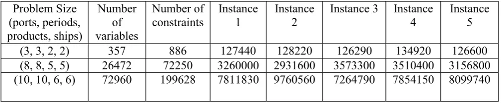
Three different problem sizes are considered to test the efficiency of the model. Table 8 presents the detailed description of each problem sizes in terms of number of ports, periods, ships and products considered. The first problem is a small size problem comprising of 3 ports, 3 time periods, 2 products and 2 ships as mentioned earlier. Six different instances are generated for this problem based on the nature of demand/supply at a port. The number of variables considered in this problem are 357. The second problem considers a scenario of 8 ports, 8 time periods, 5 products and 5 ships. 26472 number of variables are involved in this problem. The third problem deals with 10 ports, 10 time periods, 6 products and 6 ships. This can be considered as a large size problem on the basis of the number of variables (72960). Each of the aforementioned problems are solved using PSO-CP and validated using traditional PSO and GA. Total cost incurred for each instance of different problem sizes are tabulated. The visual illustrations of the convergence of the solutions are shown in the figure 11, 12. Y-axis represents the global best for each iteration. Total cost obtained at the end of each iteration is presented in the graph. Use of PSO-CP for this model is justified by the large number of variables specific to each problem used for the computation of results (as shown in table 8).
<<Insert Table 8>>
<< Insert Figure 12>>
7. Conclusion
In this paper, a mathematical model is developed addressing the sustainable ship routing problem for varying demand and supply scenario at different ports. The model is a Mixed Integer Non-Linear Programming problem considering the essence of time window, carbon emission and fuel consumption. The formulated model is solved using PSO-CP, basic PSO and GA. The sterling qualities of the algorithm employed (PSO-CP) helps to easily escape from local optima and strongly achieve near optimal point consistently which can be witnessed from the results. The results obtained from PSO-CP are completely dominating the results from the basic PSO and GA. There is a further possibilities of extending this research work by including fuel cost in the objective function. Till now the model is confined only to deterministic demands which can be considered for stochastic cases as well. Inventory replenishment decisions can be included to tackle inventory analysis scenario. The model can also be integrated with berth allocation to address more complex port operations. Moreover, the model developed in this paper can be extended to a multi objective one by considering the service time and other costs described here. It can further motivate in devising computationally efficient multi-objective algorithms for solving such problems. Insights evolved out of this article would be much beneficial for port operations and crew members. This solution would help the port authorities to readjust their schedule associated with ship routing for minimizing the transportation cost and the carbon emission.
References
Agra A, Christiansen M, Delgado A, Mixed Integer Formulations for a Short Sea Fuel Oil Distribution Problem. Transportation science, 2013; 47(1): 108-124.
Agra A, Christiansen M, Delgado A, Simonetti L, Hybrid heuristics for a short sea inventory routing problem. European Journal of Operational Research, 2014; 236(3): 924-935.
Al-Khayyal F, Hwang S-J. Inventory constrained maritime routing and scheduling for multi-commodity liquid bulk, part I: Applications and model. European Journal of Operational Research, 2007; 176(1): 106-130.
Andersson H., Fagerholt K. and Hobbesland K. Integrated maritime fleet deployment and speed optimization: Case study from RoRo shipping. Computers & Operations Research. http://dx.doi.org/10.1016/j.cor.2014.03.017
Babu S. A. K. I, Pratap S, Lahoti G, Fernandes K. J, Tiwari M K, Mount M, Xiong Y. Minimizing delay of ships in bulk terminals by simultaneous ship scheduling, stockyard planning and train scheduling. Maritime Economics & Logistics, 2015; 17(4), 464-494.
Barnhart C., Laporte G.. Handbooks in Operations Research & Management Science: Transportation. 2007, 14. 1-784. DOI: 10.1016/S0927-0507(06)14004-9.
Beheshti A. K, Hejazi A. R, Alinaghian M. The vehicle routing problem with multiple prioritized time windows: A case study. Computers & Industrial Engineering, 2015; 90(1), 402-413.
Buhaug Ø, Corbett J. J, Endresen Ø, Eyring V, Faber J, Hanayama S, Lee D. S, Lee D, Lindstad H, Markowska A. Z, Mjelde A, Nelissen D, Nilsen J, Palsson C, Winebrake J. J, Wu W. Q, and Yoshida K. Second IMO GHG Study (London, UK: International Maritime Organisation (IMO)) 2009.
Cariou P. Is slow steaming a sustainable means of reducing CO2 emissions from container shipping? Transportation Research Part D, 2011; 16(3): 260-264.
Chaug I. H. and Yu P. H. Shipping economic analysis for ultra large containership. Journal of the Eastern Asia Society for Transportation Studies. 2005; 6, 936 951.
Christiansen M. Decomposition of a combined inventory and time constrained ship routing problem. Transportation Science, 1999; 33(1): 3-16.
Corbett J.J, Köhler H.W. Updated emissions from ocean shipping. Journal of Geophysical Research, 2003; 108(20): 4650-4663.
Corbett J. J, Wang H. and Winebrake J. The effectiveness and costs of speed reduction on emissions from international shipping. Transportation Research Part D, 2009; 14(8): 539-598.
Cullinane K. and Khanna M. Economies of scale in large container ships. Journal of Transport Economics and Policy, 1999, 33 (2), 185 208.
Cóccola M. E, Méndez C. A. An iterative MILP-based approach for the maritime logistics and transportation of multi-parcel chemical tankers. Computers & Industrial Engineering, 2015; 89(1), 88-107.
Endresen Ø, Sørgard E, Behrens H.L, Brett P.O and Isaksen I. S. A. A historical reconstruction of ships fuel consumption and emissions. Journal of Geophysical Research, 2007; 112(D12), DOI:10.1029/2006JD007630.
Eyring V, Kohler H. W, Aardenne J V. and Lauer A. Emission from international shipping: 1. The last 50years. Journal of Geophysical Research, 2005; 110(D17), 306.
Grønhaug R, Christiansen M, Desaulniers G, Desrosiers J. A branch-and-price method for a liquefied natural gas inventory routing problem. Transportation Science, 2010; 44(3): 400-415.
ICS, World Trade and the Reduction of CO2 Emissions. London: International Chamber of
Shipping 2009.
IMO, MEPC 60/4/35. London: International Maritime Organization 2009a.
IMO, MEPC.1/Circ.684. London: International Maritime Organization 2009b.
IMO, Second IMO GHG Study 2009. London: International Maritime Organization 2009c.
Kachitvichyanukul V, Sombuntham P, Kunnapapdeelert S. Two solution representations for solving multi-depot vehicle routing problem with multiple pickup and delivery requests via PSO. Computers & Industrial Engineering, 2015; 89(1), 125-136.
Kontovas C, Psaraftis H N. Reduction of emissions along the maritime intermodal container chain: operational models and policies. Maritime Policy & Management, 2011, 38(4), 451-469.
Korsvik J. E., Fagerholt K. and Laporte G. A large neighbourhood search heuristic for ship routing and scheduling with split loads. Computers & Operations Research, 2011, 38(2), 474 483.
Liu L, Yang S., and Wang D. Particle Swarm Optimization With Composite Particles in Dynamic Environments. IEEE Transactions on Systems, Man, and Cybernetics Part b: Cybernetics, December 2010, 40(6): 1634-1648.
MirHassani S. A, Abolghasemi N. A particle swarm optimization algorithm for open vehicle routing problem. Expert Systems With Applications, 2011; 38(9), 11547-11551.
Notteboom, T.E.. The time factor in liner shipping services. Maritime Economics and Logistics, 2006, 8 (1), 19 39.
Repoussis P. P, Tarantilis C. D, Braysy O, Ioannou G. A hybrid evolution strategy for the open vehicle routing problem. Computers & Operations Research, 2010; 37(3), 443-445.
Ronen D. The effect of oil price on the optimal speed of ships. Journal of Operation Research Society, 1982; 33(11), 1035-1040.
Ronen D. Marine inventory routing: Shipments planning. Journal of Operation Research Society, 2002; 53(1), 108-114.
Stalhane M., Andersson H., Christiansen M., Cordeau J. F. and Desaulniers G. A branch-price-and-cut method for a ship routing and scheduling problem with split loads. Computers & Operations Research, 2012, 39(12), 3361 3375.
Tasan A. S, Gen M. A genetic algorithm based approach to vehicle routing problem with simultaneous pick-up and deliveries. Computers & Industrial Engineering, 2012; 62(3), 755-761.
Yin J, Fan L, Yang Z and Kevin X. L. Slow steaming of liner trade: its economic and environmental impacts. Maritime Policy and Management. 2014; 41(2): 149-158.
Yao Z., Ng S. H. and Lee L. H. A study on bunker fuel management for the shipping liner services. Computers & Operations Research. 2012, 39(5), 1160 1172.
Yu V. E, Jewpanya P, Redi A. A. N. P. Open vehicle routing problem with cross-docking. Computers & Industrial Engineering, 2016; 94(1), 6-17.
Zachariadis E. E, Tarantilis C. D, Kiranoudis C. T. The load-dependent vehicle routing problem and its pick-up and delivery extension. Transportation Research Part B, 2015; 71(1), 158-181.
Table 1: Swarm representation
Variable Variable Structure Number of Variables Considered
(in our experimental instances)
qkrls x
11111, 11112, 11121, 11122,... 33332
var
binary iables
x
x
x
x
x
3 3 3 3 2 162
q k r l s
qks
z 111, 112, 121, 332,
var ...
binary iables
z z z z
3 3 2 18 q k s
qk
t 11 12 13 33
vari , , ,...
continuous ables
t t t t 3 3 9
E qk
t 11 12 13 33
vari , , ,...
E E E E
continuous ables
t t t t 3 3 9
qrs
W 111 121 131 332
vari , , ,...
continuous ables
W W W W 3 3 2 18
qk
p 11 21 31 33
vari , , ,...
continuous ables
p p p p 3 3 9
qksp
O 1111 1211 1311 3322
vari , , ,...
continuous ables
O O O O 3 3 2 2 36
qksp
Q 1111 1211 1311 3322
vari , , ,...
continuous ables
Q Q Q Q 3 3 2 2 36
qksp
I 1111 1211 1311 3322
vari , , ,...
continuous ables
I I I I 3 3 2 2 36
qkp
S 111 211 311 332
vari , , ,...
continuous ables
S S S S 3 3 2 18
Table 2: Description of all the 6 instances (problem size 1)
Description of instances
(1 indicates delivery port, -1 indicates consumer port)
Instance J11 J12 J21 J22 J31 J32
1 1 -1 1 -1 1 -1
2 -1 1 -1 1 -1 1
3 1 -1 1 1 -1 -1
4 -1 -1 -1 1 1 1
5 1 -1 -1 1 1 -1
6 1 -1 -1 1 -1 1
Table 3: Table depicting the data considered for the experimental purpose
Data Set Being Considered for Experimental Instances
Parameter or variable Range Units
qr
L (300,500) Nautical Miles (nm)
qrs
W (15,30) knots
A qk
T (6,9) Hours (real time)
B qk
T (18,20) Hours (real time)
W qp
C (2,8) USD per gallon
qp
T (0.2 , 1) Minutes
qkp
D (1800,4000) Gallon per PH
qrs
C (30,80) USD per nm
s
V (2500,4000) Gallons
qp
Y (1000,3000) Gallons
qp
U (10,30) minutes
P qk
C (100,500) USD per hour
s
B (30,80) Tonnes per PH
s
F (10,30)x103 USD per PH
s
E (80,200) Tonnes per PH
qs
f (20,40) Tonnes per day
qkp
S (for k = 0) (40000,5000) Gallon per PH Planning Horizon
(PH)
Table 4: Table shows the initial ship positions (for all instances) for problem size 1
Instance 1 Instance 2 Instance 3 Instance 4 Instance 5 Instance 6
Ship 1 x21 1jn x31 1jn x21 1jn x11 1jn x31 1jn x11 1jn
Ship 2 x31 2jn x11 2jn x31 2jn x21 2jn x11 2jn x21 2jn
Table 5: Table showing different parameters and their optimal values
Parameter Inertia Weight
Acceleration coefficients
Diversification Parameter used in VAR
operation
Stretching parameters
Euclidean distance
limit
[image:25.595.67.583.549.741.2]Setting 0.9 0.1 0.98 6 2 3 0.5
Table 6: Solution obtained by using PSO-CP, PSO and tradition GA (problem size 1)
Instance Using PSO-CP Using PSO Using traditional GA
Total Cost in USD
Time of Computation
(Seconds)
Total Cost in USD
Time of Computation
(Seconds)
Total Cost in USD
Time of Computation
Table 7: Effect of carbon emission related constraints for all the 6 instances
Total Cost (considering carbon emission)
Total cost (Without considering carbon emission constraints)
% Contribution of carbon emission in Total
Cost
Instance 1 1.2744 x10⁵ 1.1746 x10⁵ 7.83% Instance 2 1.2822 x10⁵ 1.2275 x10⁵ 4.26% Instance 3 1.2629 x10⁵ 1.2210 x10⁵ 3.31% Instance 4 1.3492 x10⁵ 1.2437 x10⁵ 7.81% Instance 5 1.2660 x10⁵ 1.1328 x10⁵ 10.52% Instance 6 1.2531 x10⁵ 1.1918 x10⁵ 4.89%
Table 8: Total cost obtained for each instances of each problem size
Problem Size (ports, periods, products, ships)
Number of variables
Number of
constraints Instance 1 Instance 2 Instance 3 Instance 4 Instance 5
[image:26.595.46.551.340.446.2]Figure 1: Depicting the time window: Operating time inside and outside (with penalty) of time window
Figure 3: Flow chart depicting the construction of composite particles
[image:29.595.141.461.541.708.2]Figure 4b: Construction of composite particle using VAR scheme
[image:30.595.75.523.349.643.2]Figure 9. Graph depicts the 6 instances for problem size 1
Figure 10. Graph depicts the 6 instances for problem size 1 without considering the sustainability constraints.
[image:34.595.115.479.354.573.2]