DOI 10.1007/s10479-016-2174-8
S . I . : PATAT 2 0 1 4
A simulation scenario based mixed integer programming
approach to airline reserve crew scheduling under
uncertainty
Christopher Bayliss1 · Geert De Maere1 · Jason A. D. Atkin1 · Marc Paelinck2
© The Author(s) 2016. This article is published with open access at Springerlink.com
Abstract The environment in which airlines operate is uncertain for many reasons, for example due to the effects of weather, traffic or crew unavailability (due to delay or sickness). This work focuses on airline reserve crew scheduling under crew absence uncertainty and delay for an airline operating a single hub and spoke network. Reserve crew can be used to cover absent crew or delayed connecting crew. A fixed number of reserve crew are available for scheduling and each requires a daily standby duty start time. This work proposes a mixed integer programming approach to scheduling the airline’s reserve crew. A simulation of the airline’s operations with stochastic journey time and crew absence inputs (without reserve crew) is used to generate input disruption scenarios for the mixed integer programming simulation scenario model (MIPSSM) formulation. Each disruption scenario corresponds to a record of all of the disruptions that may occur on the day of operation which are solvable by using reserve crew. A set of disruption scenarios form the input of theMIPSSMformulation, which has the objective of finding the reserve crew schedule that minimises the overall level of disruption over the set of input scenarios. Additionally, modifications of theMIPSSMare explored, a heuristic solution approach and a reserve use policy derived from theMIPSSMare introduced. A heuristic based on the proposedMIPSSMoutperforms a range of alternative approaches. The heuristic solution approach suggests that including the right disruption
B
Christopher Bayliss [email protected] Geert De Maere [email protected] Jason A. D. Atkin [email protected] Marc Paelinck1 ASAP, University of Southampton, Southampton, UK
2 KLM Decision Support, Information services department, KLM Royal Dutch Airlines,
scenarios is as important as the quantity of disruption scenarios that are added to theMIPSSM. An investigation into what makes a good set of scenarios is also presented.
Keywords Airline reserve crew scheduling·Simulation·Mixed integer programming
1 Introduction
To maximise profits, airlines need to maximise the utilisation of resources (crew and aircraft), resulting in flight schedules with little slack. This makes each resource a critical component of an airline’s network and if a component is missing all flights related to that component may be disrupted. Crew can be absent (e.g. ill) or be delayed on connecting flights. In such circumstances airlines may call on reserve crew. This work focusses on reserve crew scheduling, i.e. determining the appropriate times at which to allocate standby reserve crew duties. In this work the possible start times for reserve crew standby duties are discretised according to the scheduled departure times of the airline’s schedule. This approach is aimed at making reserve crew recovery actions available at times as close as possible to the scheduled departure times as to minimise reserve crew induced delays.
A method has been developed called themixed integer programming simulation scenario model(MIPSSM) which will use information from repeat simulations of an airline network where reserve crew are not available. The simulation data is used to generate disruption scenarios which are used to form the constraints and coefficients of theMIPSSM formula-tion. TheMIPSSMformulation is then solved to find the reserve crew schedule that would have minimised the level of delay and cancellation that would have occurred in the original simulations (used to derive the disruption scenarios).
The remainder of the paper is structured as follows. Section2gives an overview of the proposedMIPSSMapproach. Section3outlines closely related work. Section4introduces the simulation used to generate disruption scenarios and how disruption scenarios are derived from the simulation. Section5presents the formulation of theMIPSSM and Sect.6gives several modifications and variants of the basicMIPSSM formulation including a scenario selection heuristic. Section7describes how a look up table reserve policy can be derived for a reserve crew schedule using an adapted version of theMIPSSMformulation. Section8 introduces several alternative objective functions for theMIPSSM. Section9gives exper-imental results. Section10 presents an investigation into what makes a good set of input scenarios for theMIPSSMformulation with respect to solution reliability and the quality of the resultant reserve crew schedule. Section11discusses the possible future work. Section12 concludes the paper with a summary of the main findings.
This paper adds a new approach that complements the existing literature on approaches to increasing airline schedule robustness (see Sect.3). This work focusses on the problem of reserve crew scheduling, and treats the reserve crew schedule as a means of augmenting the robustness of the airline’s crew schedule. Airline reserve crew scheduling is an important problem because of the dependencies that exist between the aircraft, crew and passenger layers of an airline’s overall schedule. Disruptions in one layer of the schedule can spread laterally to the other layers and can also be propagated (longitudinally) downstream to subsequent flights. So reserve crew can be strategically scheduled to minimise disruptions for which crew-related disruptions are the root cause.
approach applied within a different problem domain. As far as the authors are aware no previous work has used a scenario based approach for reserve crew scheduling. The proposed model is based on an airline operating a single hub airline network. The large domestic airline on whose data and practises this work is based have reserve crew stationed at their hub station who are on standby and are ready to replace disrupted crew. Disrupted crew include both absent and delayed crew. This work proposes an approach for assigning reserve crew to standby duties with the aim of minimising day of operation disruptions. The presented problem formulation is based on the case of a single crew and single fleet type. There are four reasons for doing this: (1) it simplifies the analysis of the results, allowing for a clear demonstration of how the approach can yield reserve crew schedules that minimise cancellations and delay disruptions; (2) the single crew and fleet type model still captures the main difficulty of this problem, that of modelling the uncertain demand for reserve crew; (3) the single crew and fleet type model is directly applicable to captain and first officer scheduling as these crew types are each normally qualified for a single fleet type and are usually scheduled separately (this is the case for the airline on whose operations this work is based); and (4) extending the model to a multiple crew and fleet type model is a relatively simple matter and the proposed solution approaches are directly applicable to the extended model. The implications of considering multiple fleets, crew ranks, and qualifications on the model and solution approach are discussed in more detail in Sect.11.2.
The contributions of this paper are both practical and methodological. The practical con-tributions include: the introduction of a framework for solving a challenging real world scheduling problem whose only input requirement is a simulation of the airline’s operations; and experimental results that demonstrate that this approach has the potential to minimise day of operation delay and cancellation disruptions. The methodological contributions include: a specification of how to derive disruption scenarios from the airline’s simulator; and the intro-duction of a scenario selection heuristic which is shown to be capable of deriving higher qual-ity reserve crew schedules using fewer input scenarios compared to the standard formulation.
2 Overview of the MIPSSM
This section describes the sequence of stages involved in theMIPSSMapproach. Additionally a function that converts delays into an equivalent measure of cancellations is introduced, the purpose of which is to retain the simplicity of a single objective in theMIPSSMformulation.
2.1 Stages of theMIPSSMapproach
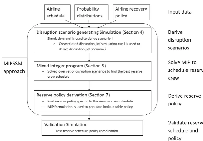
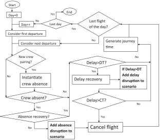
Figure1illustrates the stages that are required to be performed sequentially in the proposed MIPSSM approach, from input data through to validation. Note that the input data and validation simulation stages are not part of theMIPSSMapproach to reserve crew scheduling, but have been included in Fig.1to illustrate the full cycle of deriving and testing reserve crew schedule and policy combinations. TheMIPSSMapproach to reserve crew scheduling involves three main stages:
corre-Airline schedule
Probability distribuons
Airline recovery policy
Disrupon scenario generang Simulaon (Secon 4)
Simulaon run i is used to derive scenario i
o Crew related disrupon j of simulaon run i is used to derive disrupon j of scenario i
Mixed Integer program (Secon 5)
Solved over set of disrupon scenarios to find the best reserve crew schedule
Reserve policy derivaon (Secon 7)
Find reserve policy specific to the reserve crew schedule MIP formulaon is used to populate look up table policy
Validaon Simulaon
Test reserve schedule policy combinaon
Input data
Derive disrupon scenarios
Solve MIP to schedule reserve crew
Derive reserve policy
Validate reserve schedule and policy MIPSSM
approach
Fig. 1 Sequential stages of the proposed approach to scheduling airline reserve crew
sponding record of all of the reserve crew start times (discretised to match the scheduled departure times) which, if scheduled, would allow the corresponding reserve crew to be used to remove completely, or reduce, the given disruption.
2. AMIPSSM formulation is solved to find the best reserve crew schedule for the set of disruption scenarios generated in the first stage. In theMIPSSM formulation there are two types of variables:x the reserve crew schedule andythe reserve use variables. For each disruption scenario there is a corresponding subset of the reserve use variables. The reserve use decisions made for each disruption scenario have to be feasible with respect to the overall reserve schedulex(i.e. reserve crew can only be used if they are scheduled). The difficulty is finding a reserve schedule that allows disruptions in many scenarios to be covered in an efficient manner. Solving theMIPSSMformulation over a set of input disruption scenarios in an appropriate solver finds both the reserve crew schedulexand the reserve use decisionsythat together minimise delay and cancellations over all of the input disruption scenarios.
3. Lastly, a reserve policy is derived, corresponding to the reserve crew schedule found in theMIPSSM formulation stage, which defines the conditions on the day of operation under which reserve crew use is permitted. The policy takes the form of a look up table which specifies the minimum number of reserve crew that should be available at each departure time if reserve crew are to be permitted to be used to absorb crew-related delay affecting a given departure.
2.2 Cancellation measure of a delay
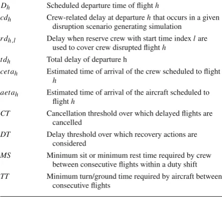
[image:4.439.46.382.49.283.2]Table 1 Cancellation measure
and related notation Dh Scheduled departure time of flighth
cdh Crew-related delay at departurehthat occurs in a given disruption scenario generating simulation
r dh,l Delay when reserve crew with start time indexlare
used to cover crew disrupted flighth tdh Total delay of departure h
cetah Estimated time of arrival of the crew scheduled to flight h
aetah Estimated time of arrival of the aircraft scheduled to
flighth
CT Cancellation threshold over which delayed flights are cancelled
DT Delay threshold over which recovery actions are considered
MS Minimum sit or minimum rest time required by crew between consecutive flights within a duty shift
TT Minimum turn/ground time required by aircraft between consecutive flights
formulation, Eq.1converts delay into a measure of cancellation. The simulation cancels flights with a delay over the cancellation threshold so the maximum cancellation measure of a delay is 1. Table1defines the notation required for calculating delays and delay cancellation measures.tdh (Eq.2) is the total delay of flighth,cdh (Eq.3) is the delay of flighthdue
to crew over and above delay due to the aircraft, i.e. the delay which could be absorbed by using reserve crew. Equation4gives the total delay that occurs when reserve crew with start time indexl(start time= Dl as reserve start times are discretised according to scheduled
departure times) are used to replace the delayed connecting crew of flighth. The cancellation measure associated with using reserve crew can still be calculated from Eq.1by replacing the numerator by Eq.4.
cmh =
tdh−cdh
CT
n
(1)
tdh =max(0,max(aetah+T T,cetah+M S)−Dh) (2)
cdh =max(0,cetah+M S−max(Dh,aetah+T T)) (3)
r dh,l =max(0,max(Dl,aetah+T T)−Dh) (4)
The particular choice ofn=2 permits a balanced demonstration of how this work accounts for delay and cancellation disruptions. Note however that any value ofncould be used.
The disruption scenario generation stage collects information about the possible objective value (cancellation measures) of using reserve crew scheduled at different times for different disruptions in each disruption scenario.
2.3 Disruption scenarios
The proposedMIPSSM approach uses the concept of disruption scenarios. A disruption scenario corresponds to a set of crew-related disruptions that could occur during the imple-mentation of an airline’s schedule. In the MIPSSM approach, disruption scenarios are collected from a simulation of an airline. The simulation has stochastic crew absence and journey time inputs instantiated from corresponding statistical distributions. For each disrup-tion in a disrupdisrup-tion scenario informadisrup-tion must be maintained about the disrupdisrup-tion size (in the form of a cancellation measure), the number of reserve crew required to cover the disruption, and the benefits of using reserves crew scheduled at different times to cover the disruption. The information about the benefit of using reserves scheduled at different possible times is stored in the form of sets offeasible reserve instancescorresponding to each disruption in each disruption scenario (see Sect.2.4)
2.4 Feasible reserve instances
In the simulation which generates disruption scenarios, information regarding the benefit of using reserve crew scheduled at different times to absorb a given disruption is collected. For each reserve start time that is feasible to absorb a given disruption, afeasible reserve instanceis generated. A feasible reserve instance therefore corresponds to a combination of a reserve crew duty start time and a disruption that could be absorbed by using a reserve crew with such a duty start time. For each feasible reserve instance there is a cancellation measure which replaces the cancellation measure of the original disruption if the reserve is used (in the MIPSSM formulation) to cover the disruption. The use of feasible reserve instances means that theMIPSSMformulation only contains binary variables corresponding to feasible reserve crew which can, if scheduled, be used to cover disruptions. Reserve feasibility constraints are therefore not required as only feasible reserve recovery actions are included in theMIPSSM formulation.
Letbdenote a given feasible reserve instance. For each feasible reserve instance there is:
1. A corresponding cancellation measure (CM(b)) which is calculated in the disruption scenario generation stage. This is the cancellation measure that applies in theMIPSSM formulation if reserve crew with the duty start time (corresponding tob) are used to cover the disruption (corresponding tob).
2. An associated unique reserve use variable index (V(b)) which identifies the binary reserve use variable in the MIPSSM formulation associated with the feasible reserve instance.
3. A unique (knock-on effect) reserve use variable index (U(b)) corresponding to feasible reserve instances which can absorb a root delay that subsequently propagates, hence reducing the secondary delay.
Feasible reserve instances generated in the disruption scenario generation phase are each stored in two sets. In one set containing all of the feasible reserve instances which were generated for the same disruption and the same disruption scenario, and in a second set containing all of the feasible reserve instances generated with the same reserve start time and for the same disruption scenario. These sets are then used to form the constraints of the MIPSSMformulation (Sect.5).
3 Related work
TheMIPSSMapproach has similarities to recoverable robustness as introduced byLiebchen et al.(2007). Recoverable robustness provides a framework for timetabling problems with the objective that the schedule must be feasible in each of a limited set of disruption scenar-ios given limited availability of recovery from disruptions. Their approach reduces to strict robustness (feasible in all outcomes without recovery actions) if the feature of limited avail-able recovery is removed. The similarity between recoveravail-able robustness and theMIPSSM approach lies in the idea of solving a scheduling problem over a limited number of realistic disruption scenarios, but differs because recoverable robustness assumes a fixed capacity for recovery exists whereas in this work the recovery action is what is being scheduled. The MIPSSMapproach is influenced by stochastic programming, which optimises over a set of explicit independent possible outcomes as opposed to optimising over the expected outcome, which may not even correspond to a possible outcome.
There has been relatively little work on reserve crew scheduling in the past and none looks at exactly the same problem.Sohoni et al.(2006) present an airline reserve crew scheduling model that takes training days and bidline conflicts into account. Such conflicts arise when crew bid for rosters which overlap with recurring training and this leads to open time (flights without scheduled crew) which have to be covered with reserve crew. The work of Sohoni et al. primarily focusses on scheduling reserve crew in anticipation of reserve crew demand from scheduling conflicts due to reoccurring training, less attention is given to reserve demand due to day of operation disruption, which is the main focus of this work. The work ofBoissy (2006) describes an absenteeism forecast model and a model for minimising the cost of reserve crew and missing crew. Boissy defines tension as the number of disruptions divided by the number of reserve crew, using more reserve crew decreases tension but increases the crew cost. Boissy’s model is used to find the optimal tension, which corresponds to the minimum cost of missing crew plus reserve crew cost. Boissy’s main focus is manpower planning whereas in this work the focus is on the scheduling of the available manpower. Dillon and Kontogiorgis(1999) present an approach for pilot reserve crew scheduling that generates reserve pairings which are then subject to crew bidding. They focus on quality of life considerations such as regularity. Their work helped in negotiations with pilot unions. The work of Dillon and Kontogiorgis refers to the specific case of US airlines, who have permanent reserve crew who are used to fill open or disrupted pairings. Open pairings are crew pairings that do not have crew assigned. Dillon and Kontogiorgis generate call out day pairings for reserve crew and focus on generating pairings with regularity and varying lengths. Generating varying length pairings allows for reserve crew who have different amounts of time off in a given month. In contrast to Dillon and Kontogiorgis, in this work reserve crew pairings are all regular as they start at the same time every day, and also have fixed lengths, since this is the way that KLM operate.
reserve crew and the expected number of reserve crew remaining each day, and uses a reserve block stacking approach. The aim is to always have standby reserve crew available.Paelinck (2001) also highlights some of the difficulties associated with the planning and scheduling of reserve crew, including how many should be scheduled, when and what is the best way to use them in response to disruptions.
As described in Sect.1a reserve crew schedule augments the robustness of an already existing crew schedule.Shebalov and Klabjan (2006) increase crew schedule robustness using the concept of move-up crews. Move-up crews refers to crews who can swap pairings in the event of delay (the available crew can adopt the delayed crew’s pairing). Their objec-tive is to maximise the availability of move-up crews. Shebalov measures the robustness of schedules/quality of the scheduled move-up crews in computational experiments in terms of the number of deadheads (crew transported as passengers to the origin of their next flight leg), reserve crew used, number of uncovered flight legs and the cost of the crew schedule. The simulation used in theMIPSSMapproach includes crew swap recovery actions, and therefore theMIPSSMapproach takes the pre-existing robustness of the crew schedule into account. This means that if the input crew schedule for theMIPSSMwas derived from an approach such as that of Shebalov and Klabjan, theMIPSSMwould preserve the increased schedule robustness which was introduced by their approach and add extra schedule robustness. On a similar note, the approach ofAgeeva and Clarke(2000) was to increase the availability of swap recovery actions by encouraging ground time overlaps, whilstSmith(2004) did the same for aircraft swap opportunities (using the concept of station purity).
Other work on increasing airline schedule robustness, which is complementary to that proposed in this work, has also been carried out.Sohoni et al.(2011) introduce stochastic programming models for modifying airline schedule departure times within allowable time windows, with the aim of increasing on-time performance and minimising the probability of passengers missing connections.Weide et al.(2010),Dunbar et al.(2012) andDuck et al. (2012) took the approach of performing crew pairing and aircraft routing in an integrated fashion, which helped to reduce disruptions resulting from dependencies between the crew and the aircraft schedules. These complementary approaches, including theMIPSSM, to increasing airline schedule robustness can all be applied during the applicable planning phases, the result of which will be even greater schedule robustness.
TheMIPSSMapproach uses simulation to obtain information about the most beneficial times to schedule standby reserve crew. Simulation has also been used to determine opera-tional crew costs for an airline crew pairing problem. In particular,Rosenberger et al.(2002) use a simulation approach to replace planned pairing costs with operational costs. The reason-ing behind such approaches is that minimisreason-ing planned costs is an optimistic approach (i.e. assuming no disruptions leads to fragile schedules), whereas the operational cost based solu-tion, despite costing more than the planned cost, will on average cost less after the recovery costs are added to the planned costs. In experiments they show that their approach minimises expected crew costs compared to state of the art approaches based on planned costs.
considers disruption scenarios that are in progress, whereas as in this work many possible future disruption scenarios are generated in order to find a single reserve crew schedule that works well in all of them.
The work ofBayliss et al.(2012) introduced a probabilistic model of crew absence and reserve crew used to cover absence. The approach was based on the knowledge of the prob-abilities of crew absence for each flight in an airline’s schedule. The probabilistic model evaluated the effect a given reserve crew schedule has on the probabilities of cancellations due to crew absence. The solution space of reserve crew schedules was then searched to find the reserve crew schedule that minimised the probabilities of cancellations due to crew absence. It was found that constructive heuristics provided near optimal solutions when solv-ing the model presented inBayliss et al.(2012) whilst a hybrid dynamic programming and branch and bound heuristic approach was able to find the optimal solutions. In contrast to Bayliss et al.(2012) this work investigates the alternative approach of modelling reserve demand uncertainty using a scenario based approach rather than a probabilistic model.
4 Disruption scenario generation simulation
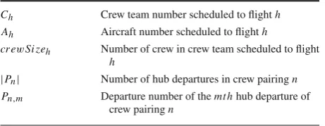
This section explains the disruption scenario generation stage of theMIPSSMapproach. Sec-tion4.1gives details of the single hub airline simulation, which is used firstly for disruption scenario generation and then later reused for experimental validation of reserve crew sched-ules. Section4.2defines what is meant by a disruption scenario and how the information it stores is collected from the simulation. Table2defines the input airline schedule notation. Table3defines the notation used for disruption scenarios.
4.1 Simulation
The simulation of a single hub airline is used without reserve crew to generate a set of disruption scenarios which contain information on the possible benefit of using reserve crew scheduled at specified times to mitigate the the given disruption. These disruption scenarios form the input for theMIPSSMformulation (Sect.5.1).
Simulation takes as input the airline’s scheduled flights and the crew and aircraft which are scheduled to each of those flights. The simulation’s stochastic inputs are journey times and crew absence, each of which have corresponding statistical distributions derived from real data. Crew and aircraft were scheduled using first in first out scheduling (see Sect.9.1 for details of the test schedule instance).
[image:9.439.166.397.528.617.2]The simulation has a dual purpose: disruption scenario generation and reserve crew sched-ule validation. For disruption scenario generation, no reserve crew are schedsched-uled and none are
Table 2 Schedule notation
Ch Crew team number scheduled to flighth Ah Aircraft number scheduled to flighth
cr ewSi zeh Number of crew in crew team scheduled to flight h
|Pn| Number of hub departures in crew pairingn Pn,m Departure number of themt hhub departure of
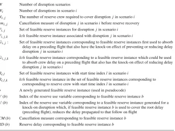
Table 3 Disruption scenario notation
W Number of disruption scenarios
Wi Number of disruptions in scenarioi
Ni,j The number of reserve crew required to cover disruptionjin scenarioi cmi,j Cancellation measure of disruptionjin scenarioibefore reserve recovery Fi,j Set of feasible reserve instances for disruptionjin scenarioi
Fi,j,k kt hfeasible reserve instance associated with disruptionjin scenarioi
Gi,j: Set of feasible reserve instances corresponding to feasible reserve instances first used to absorb
delay on a preceding flight that also have the knock-on effect of preventing or reducing delay disruption jin scenarioi
Gi,j,k kt hfeasible reserve instance corresponding to a feasible reserve instance which could be used
to absorb crew delay on a preceding flight that also has the knock-on effect of reducing delay disruption jin scenarioi
Ri,l Set of feasible reserve instances with start time indexlin scenarioi
Ri,l,k kt hfeasible reserve instance in the set of feasible reserve instances corresponding to
corresponding to reserve crew with start time indexlin scenarioi b A newly generated feasible reserve instance (used in pseudocode)
V(b) Index of the reserve use variable corresponding to feasible reserve instanceb
U(b) Index of the reserve use variable corresponding to a feasible reserve instance generated for a knock-on disruption which, if feasible reserve instancebis used to cover the root delay (preceding flight), reduces the delay propagated to that follow on flight
CM(b) Cancellation measure corresponding to feasible reserve instanceb RD(b) Reserve delay corresponding to feasible reserve instanceb
therefore available for recovery (as the point of disruption scenario generation is to find infor-mation about when reserve crew are most needed). In contrast the validation simulation does include a reserve crew schedule and is used to compare the reserve crew schedules which were found using theMIPSSM against reserve crew schedules obtained using alternative approaches.
Day=0
Consider next departure
No
Yes
Instanate crew absence
Yes
No
Yes
No
Cancel flight
Yes
Delay recovery
Crew absent?
New crew pairing?
Absence recovery?
Delay>DT?
Delay>CT?
Yes
Generate journey
me
No
Last flight
of the day?
No Yes
Last day
Yes No
No
If Delay>DT Add delay disrupon to scenario Day++
Add absence disrupon to scenario
End Start
Consider first departure
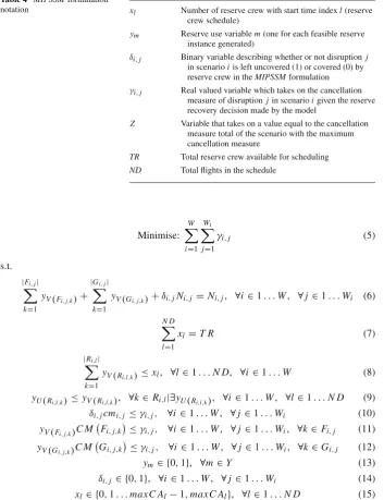
Fig. 2 Flow chart of the simulation used to derive disruption scenarios
each other’s duties without violating maximum working hours and it must be possible to undo the swap in the overnight break (i.e. the crew must stay overnight at the same station). In the disruption scenario generation simulation, if the delay is still above the delay threshold even after the consideration of swap recovery actions, information is collected on the possible benefit of scheduling reserve crew at different possible start times (Sect.4.2). The validation simulation also considers reserve crew as a possible recovery action from delays. If the delay is still above the cancellation threshold (180 minutes) the flight is cancelled.
4.2 Simulation derived scenarios
A given disruption scenarioi corresponds to a single run of the simulation. This section explains how simulation is used to derive the information for disruption scenarios.
In disruption scenarioi, a disruption j corresponds to the j t hcrew disrupted flight for which reserve crew use could be a beneficial recovery action. Reserve crew use is beneficial when a flight either has a delay which is greater than the delay threshold (the minimum delay that is considered a delay worth recovering from), even after the consideration of swap recovery, or has to be cancelled due to crew absence. Such disrupted flights have a positive cancellation measure, wherecmi,jdenotes the cancellation measure of disruptionj
in disruption scenarioi.
[image:11.439.65.378.54.327.2]Algorithm 1Pseudocode for deriving disruption scenario information for a crew absence disruption occurring at simulation runideparturek
1: Inputs: Crew-related disruption affecting departurekof simulation runi(number of absent crew) 2: Outputs: Disruptionjof scenarioi(cmi,j,Ni,j,Fi,j. . .)
3: RU V I=number of reserve use variable indices used so far 4:ifcrew absence disruptionthen
5: Wi=Wi+1
6: Ni,j=number of crew absent
7: cmi,j= |PCk|(all hub departures cancelled if absence is not covered)
8: forl=1 to total hub departuresdo
9: form=1 to|PCk|do
10: ifreserve crew with start timeDlare feasible to cover crew absence at themt hhub departure of the
crew pairing assigned to crew team numberCkthen
11: f =PCk,m(m
t hflight of the crew pairing assigned to flightk)
12: cm=m−1+r dC Tf,l
n
(number of cancellations before reserve with start time indexlcan be used plus cancellation measure due to reserve induced delay when reserve is first used) 13: forn=1 toNi,jdo
14: b=new feasible reserve instance 15: C M(b)=cm
16: V(b)=RU V I(index of new feasible reserve instance) 17: Fi,j=Fi,j∪b
18: Ri,l=Ri,l∪b
19: RU V I=RU V I+1 20: end for
21: end if
22: end for
23: end for
24: j=j+1 25:end if
feasible reserve instances are generated. A feasible reserve instance (Sect.2.4) corresponds to a feasible reserve crew duty start time index which can be used to cover a given crew disrupted flight in a given scenario (i.e. reserve start time/disruption pair). For each disruption the number of feasible reserve instances which are generated for each feasible reserve start time index is equal to the number of reserve crew required to cover the given disruption, which is either the number of crew absent (for a crew absence disruption) or the size of the crew team assigned to flighth(cr ewSi zeh) for a delay. LetFi,j denote the set of feasible
reserve instances corresponding to possible reserve start times that could, if scheduled, be used to solve or reduce disruptionjof disruption scenarioi.
For the specific case of delay disruptions it is also possible that reserve crew use can have the effect of reducing or preventing knock-on delays. For this purpose the setGi,j is introduced which denotes the set of feasible reserve instances corresponding to the possible use of reserve crew which were originally used to absorb the root delay also being used to absorb the knock-on disruption. Note that crew-related delays occur when a flight has to wait for crew on a delayed connecting flight, so the reserve used for the root delay can only influence the delay of the following flight if other reserve crew are not used to absorb the delay of that following flight. Algorithms1and2outline the procedure of collecting information for the disruption scenarios from the single hub airline simulation.
Algorithm1is used in the disruption scenario generating simulation when a crew absence occurs, the algorithm considers all of the possible ways the absence disruption can be covered using reserve crew (reserve crew with different start time indicesl) and generatesNi,jfeasible
Algorithm 2Pseudocode for deriving disruption scenario information for a crew delay dis-ruption occurring at simulation runideparturek
1: Inputs: Crew-related disruption affecting departurekof simulation runi(number of absent crew) 2: Outputs: Disruptionjof scenarioi(cmi,j,Ni,j,Fi,j,Gi,j. . .)
3: RU V I=number of reserve use variable indices used so far 4:ifcrew delay disruptionthen
5: Wi=Wi+1 6: Ni,j=cr ewSi zek
7: cmi,j= td
k C T
n
8: forl=1 to total hub departuresdo
9: ifreserve crew with start timeDlare feasible to absorb crew-related delay of departurekthen
10: cm=r dC Tk,ln
11: forn=1 toNi,jdo
12: b=new feasible reserve instance 13: C M(b)=cm
14: V(b)=RU V I
15: Fi,j=Fi,j∪b
16: Ri,l=Ri,l∪b
17: RU V I=RU V I+1 18: end for
19: end if
20: end for
21: ifcurrent crew delay is crew delay propagated from the crew’s previous flightthen
22: q=crew’s previous flight 23: o=disruption number of flightq
24: forl=1 to|Fi,o|do
25: cm=
max0,tdk−tdq−R DFi,o,l C T
n
(cancellation measure of the propagated delay if feasible reserve instanceFi,o,lis used to absorb the root delay)
26: b=new feasible reserve instance 27: C M(b)=cm
28: V(b)=RU V I
29: UFi,o,l=RU V I(reference to the knock-on effect reserve use variable)
30: Gi,j=Gi,j∪b
31: RU V I=RU V I+1 32: end for
33: end if
34: j=j+1 35:end if
the number of absent crew (line 6). The cancellation measure of the absence disruption is the number of hub departures in the disrupted crew pairing that would have to be cancelled if reserve crew were unavailable to cover the absent crew (line 7), with no delay contribution to the cancellation measure.
and scenario they are applicable to (line 18). These sets are useful later on when creating the constraints for feasible reserve use in theMIPSSMformulation.
Algorithm2is used in the disruption scenario generating simulation when a crew-related delay occurs. The algorithm stores the size of the disruption and then considers all of the possible reserve crew recovery actions and generates feasible reserve instances for each. Algorithm2differs from Algorithm1because of the type of disruption (delay rather than absence) and because of the possibility that, if they were used, feasible reserve instances generated for previous crew delay disruptions in the same simulation run could have reduced the current delay. If the current crew-related delay is a delay propagated from a previous crew-related delay, feasible reserve instances are generated corresponding to the reserve crew which could have been used to absorb the root crew-related delay and are being used to cover the knock-on delay also. These feasible reserve instances are stored in the setGi,j. The number of reserve crew required to cover the given disruption in Algorithm2is the number of crew in the delayed crew team (line 6). The cancellation measure of the delay disruption when reserve crew are not available to cover the delayed crew is computed on line 7. The algorithm then considers each possible reserve start time (line 8) which could be used to cover the delay. If the reserve start time is feasible (line 9) and can absorb the delay, thenNi,j
(=cr ewSi zek) new feasible reserve instances are generated (line 11) with unique reserve
use variable indices and cancellation measures as calculated on line 10.
Lines 21 to 33 of Algorithm2apply if feasible reserve instances generated for the previous flight prevent or reduce the delay propagated to the current flight. For such feasible reserve use instances (line 24)UFi,o,l(line 29) stores a new unique reserve use variable index corresponding to the same reserve being used to absorb the delay of the following flight. The reason why an extra reserve variable index is generated for the same reserve used on a following flight is that it is possible that other reserve crew might instead be used to cover the knock-on delay if the reserves used for the root crew-related delay do not absorb all of the delay and some delay can still propagate. The setG stores feasible reserve instances corresponding to the feasible reserve instances which were generated for the root crew-related delay. Line 25 calculates the corresponding cancellation measures for these feasible reserve instances, which depend upon the amount of delay that would have propagated if the feasible reserve instance corresponding to the root crew delay was utilised. TheMIPSSM has constraints that ensure that the beneficial knock-on effects can only apply if the reserve is actually used to absorb the root crew delay.
5 The MIPSSM’s mixed integer programming formulation (MIPSSM
formulation)
This section explains the mixed integer linear programming formulation. Section5.1presents and explains the objective and constraints and Table4defines the notation used.
5.1 Mixed integer programming formulation (MIPSSM formulation)
Table 4 MIPSSMformulation
notation xl Number of reserve crew with start time indexl(reserve
crew schedule)
ym Reserve use variablem(one for each feasible reserve instance generated)
δi,j Binary variable describing whether or not disruptionj
in scenarioiis left uncovered (1) or covered (0) by reserve crew in theMIPSSMformulation
γi,j Real valued variable which takes on the cancellation
measure of disruptionjin scenarioigiven the reserve recovery decision made by the model
Z Variable that takes on a value equal to the cancellation measure total of the scenario with the maximum cancellation measure
TR Total reserve crew available for scheduling
ND Total flights in the schedule
Minimise:
W
i=1 Wi
j=1
γi,j (5)
s.t. |Fi,j|
k=1
yV(Fi,j,k)+ |Gi,j|
k=1
yV(Gi,j,k)+δi,jNi,j =Ni,j, ∀i ∈1. . .W, ∀j ∈1. . .Wi (6)
N D
l=1
xl=T R (7)
|Ri,l|
k=1
yV(Ri,l,k)≤xl, ∀l∈1. . .N D, ∀i∈1. . .W (8)
yU(R
i,l,k)≤yV(Ri,l,k), ∀k∈Ri,l|∃yU(Ri,l,k), ∀i∈1. . .W, ∀l∈1. . .N D (9) δi,jcmi,j ≤γi,j, ∀i∈1. . .W, ∀j∈1. . .Wi (10)
yV(Fi,j,k)C MFi,j,k
≤γi,j, ∀i ∈1. . .W, ∀j∈1. . .Wi, ∀k∈Fi,j (11)
yV(Gi,j,k)C MGi,j,k
≤γi,j, ∀i∈1. . .W, ∀j ∈1. . .Wi, ∀k∈Gi,j (12)
ym∈ {0,1}, ∀m∈Y (13)
δi,j ∈ {0,1}, ∀i∈1. . .W, ∀j ∈1. . .Wi (14)
xl∈ {0,1. . .maxC Al−1,maxC Al}, ∀l∈1. . .N D (15)
total number of reserve crew available (TR) are scheduled. Constraint8ensures that in each disruption scenario the number of reserve crew used with the same start time index does not exceed the number of reserve crew which are scheduled to that start time index. Constraint9 ensures that knock-on delays can only be absorbed by reserve crew if those reserve crew are actually used to cover the root delay. Constraints10to12ensure that the cancellation measure associated with a given disruption is the maximum of that associated with the recovery actions used for the given disruption. If no reserve crew are used for a given disruption, that disruption gets the cancellation measurecmi jthat occurred in the simulation run in which the disruption
occurred. If reserve crew are used, the cancellation measure is that for the reserve crew used for that disruption that invokes the largest cancellation measure (as the flight can’t take off before all of the crew are present). Constraints13to15are the integrality constraints.
6 Variants and modifications of the MIPSSM formulation
This section firstly considers 2 alternative objective functions for the basicMIPSSM formu-lation given in Eqs.5–15. Then a scenario selection heuristic is introduced which is designed to address the question of whether the types of scenarios or the number of scenarios included in the formulation has the greatest effect on solution quality.
6.1 Alternative objectives for the MIPSSM
6.1.1 MiniMax 1
The objective of minimising the sum of cancellation measures over all disruption scenarios included in the model (Objective5) could be replaced with the alternative objectiveMiniMax1 of minimising the largest sum of cancellation measures for any scenario. This is a minimax objective function, discussed in Williams (2002), and can be implemented by replacing Objective5with Objective16and adding Constraint17. This approach will have the effect of finding a reserve crew schedule that minimises the extent of the worst case scenario as opposed to minimising the average cancellation measure.
min:Z (16)
Wi
j=1
γi,j ≤Z, ∀i∈1. . .W (17)
6.1.2 MiniMax 2
Instead of minimising the total cancellation measure of the disruption scenario with the largest cancellation measure, the same principle can be applied to individual scenarios with the alter-native objectiveMiniMax2. I.e. find the reserve crew schedule that minimises the single largest disruption. To implement this approach replace Constraint set17with Constraint set18.
In the results (Table5) there is no performance measure which is directly relevant to the MiniMax2formulation because in the reserve crew schedule validation simulation the worst single disruption is a cancellation and these will inevitably occur in each method. However in theMiniMax2formulation the worst single disruption is leaving an absence disruption uncovered which would result in all flights on the absent crew’s line of flight being cancelled.
Algorithm 3Psuedocode for the scenario selection heuristic 1:newScenar i oF ound=tr ue
2:i ts=0
3:whilenewScenar i oF ound∧i ts≤i t Li mdo
4: newScenar i oF ound= f alse
5: r pts=0
6: while¬newScenar i oF ound∧r pts<r pt Li mdo
7: Run simulation to generate disruption scenarionewScenar i o
8: Solve new scenario subproblem 9: ifsubObj>maxj(master Objj)then
10: newScenar i oF ound=true
11: add new scenario to the master problem 12: else
13: r pts=r pts+1 14: end if
15: ifnewScenar i oF oundthen
16: resolve master problem 17: end if
18: end while
19: i ts=i ts+1 20:end while
[image:17.439.47.394.289.444.2]21: return solution
Table 5 Performance measure averages from 20 repeats Method name Average
cancellation measure
Average delay/mins
Probability of delay>30 mins
Cancellation rate
Reserve utilisation rate
Solution time/mins
N o Res 15.009 11.147 0.00682 0.03925 – –
MIPSSM 1.159 12.180 0.00898 0.00140 0.674 28.688
MiniMax1 1.246 12.393 0.00938 0.00154 0.666 7.060
MiniMax2 1.724 13.874 0.01114 0.00171 0.656 2.259
SSH 1.066 11.870 0.00871 0.00141 0.667 2.871
Pr ob 1.077 11.518 0.00818 0.00166 0.690 0.443
Ar ea 2.399 14.001 0.01130 0.00353 0.589 0.060
USR 2.925 14.970 0.01336 0.00438 0.555 <0.001
zer os 3.756 11.167 0.00725 0.00902 0.571 <0.001
6.2 Scenario selection heuristic
The basicMIPSSMand the two alternative formulationsMiniMax1andMiniMax2are solved over a given set of disruption scenarios in a linear programming solver (CPLEX in this case). Although CPLEX yields optimal solutions, the solutions are only optimal for the set of disruption scenarios considered in the model. This section introduces a scenario selection heuristic (SSH) to address the issue of the choice of scenarios which should be included in theMIPSSM formulation. The solution time increases sharply as the number of disruption scenarios increases, which provides another motivation for considering a scenario selection heuristic solution approach, which includes the right scenarios rather than ensuring that plenty of disruption scenarios are included in the model.
is larger than the objective contribution of the scenario already in the master problem with the largest objective contribution (maxj(masterObjj)). The sub-problem objective value of a new scenario is calculated (line 8) from theMIPSSMformulation with the new scenario as the only input disruption scenario and with the incumbent reserve crew schedule (X) fixed. This heuristic is analogous to column generation in which the master problem and pricing problem are solved iteratively. In summary, this scenario selection approach focusses on finding a reserve schedule that can cope with a wide variety of difficult scenarios as opposed to a random set of scenarios representing the average outcome. This scenario selection heuristic can be expressed by Algorithm3.
7 Optimal reserve use policy derivation
This section introduces an approach for deriving an optimal reserve use policy for a given reserve schedule, by solving theMIPSSMformulation for a fixed reserve schedule repeatedly, over a single disruption scenario, at a time and learning the circumstances in which reserve crew use is eventually beneficial in the long run. The policy is optimal only in the sense that it is learned from the optimal decisions for a given set of disruptions scenarios which are solved by theMIPSSM
The simulation (Sect.4.1) which is used to test reserve schedules has a default policy of using reserve crew whenever this is immediately beneficial. The default policy also uses reserve crew in earliest start time order, so as to leave the largest amount of unused reserve crew capacity available for subsequent disruptions. TheMIPSSMapproach uses reserve crew in each disruption scenario in an optimal way based on full knowledge of future disruptions. Knowledge of future disruptions is not available in the simulation, if a scenario which was included in theMIPSSMformulation is repeated in the validation simulation, reserve crew might not necessarily be used in the same optimal way.
The reserve policy derived from theMIPSSMformulation is based on reserve use decisions in response to delayed crew, where a team of reserve crew could be constructed and used to absorb the delay. The policy consists of threshold minimum numbers of reserve crew remaining for each departure for which using reserve teams to absorb crew-related delay is deemed globally beneficial. The threshold values are calculated by repeatedly solving the reserve use variables of theMIPSSM for different disruption scenarios with the given reserve crew schedule fixed. The threshold value for a given flight is the average number of reserve crew remaining immediately before that flight if reserve crew were used in the way recommended by theMIPSSMformulation.
The default policy is used for reserve crew use in response to crew absence since the penalty for not replacing absent crew with reserve crew is cancellation. In general, using teams of reserve crew to cover delayed connecting crew is expensive as it solves a smaller disruption (a delay compared to a cancellation) using more reserve crew than are usually required to cover absent crew. However in certain circumstances using teams of reserve crew to cover delayed connecting crew can be globally beneficial. .
8 Alternative methods
8.1 Probabilistic reserve crew scheduling under uncertainty
the work inBayliss et al.(2012) to account for different numbers of crew being absent from each crew pairing in an airline schedule. Moreover the constraint that reserve crew are only feasible for disruptions if their duty start time is no later than the scheduled departure time of the disrupted flight has been relaxed so that some reserve delay is permitted, just as in theMIPSSM. Reserve delays in the probabilistic approach are accounted for using the delay cancellation measure (Eq.1).
8.2 Area under the graph
The area under the graph (Ar ea) method is based on running a number of simulations and recording the cumulative demand for reserve crew with respect to time in the form of a bar chart (in terms of the cancellation measure that could be avoided if reserve crew were available). Reserve crew are then scheduled at equal area intervals under the reserve demand graph over the whole time horizon. The Ar eaapproach is based on a simulation without reserve crew to find reserve demand independent of the effects of a reserve crew schedule.
8.3 Uniform start rate
The uniform start rate method (USR) schedules reserve crew at equal time intervals.
8.4 Zeros
TheZ er osmethod schedules all reserve crew to begin standby duties at the first departure of the first day.
9 Experimental results
TheMIPSSM(Sect.5.1),MiniMax1andMiniMax2(Sect.6.1) andSSH(Sect.6.2) approaches are tested and compared to one another. IBM CPLEX Optimization Studio version 12.5 with Concert technology is used as the MIP solver, on a desktop computer with a 2.79 GHz Core i7 processor and 6 Gb of RAM. These methods are also compared to the alternative methods for reserve crew scheduling (described in Sect.8).
9.1 Experiment design
connecting crew. The following section investigates the effect of the number of reserve crew available for scheduling for each solution approach.
9.2 Investigating the effect of varying the number of reserve crew available for scheduling
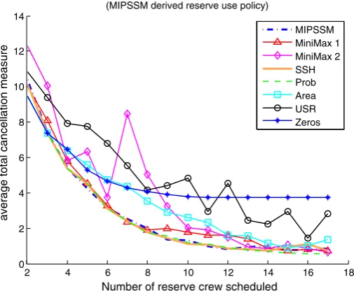
The results in Fig.3show the effect on the average cancellation measure of varying the number of reserve crew available for scheduling, using 20,000 repeat validation simulations for the reserve crew schedules from each solution approach. TheMIPSSMbased approaches are restricted to 50 input disruption scenarios and a maximum of 1 h to find a solution.
Figure3shows how the various reserve crew scheduling approaches compare for different numbers of reserve crew available for scheduling. TheSSH,MIPSSMandPr obapproaches obtain the lowest average cancellation measures of those tested for all numbers of available reserve crew. The Pr ob model gives a smooth curve of average cancellation measures, whereasMIPSSMandSSH have small fluctuations in average cancellation measure as the number of reserve crew available for scheduling changes. This fluctuation can in part be attributed to the limited number of disruption scenarios used as input for these methods. The MiniMax1modification generally leads to higher average cancellation measures especially when between 9 and 12 reserve crew were available for scheduling.MiniMax2 gave the unexpected result that scheduling more reserve crew can lead to a higher average cancellation measure. This fluctuating behaviour of theMiniMax2modification was also observed to a lesser extent in the other methods based on theMIPSSM(as well as theMIPSSMapproach itself) and can be explained by the fact that the objective of theMiniMax2modification is to suppress the single largest delay or cancellation disruption that can occur and is not to minimise the average cancellation measure. This fluctuation is due to the resultant schedules being designed for worst case disruptions as opposed to the average outcomes. The Ar ea
2 4 6 8 10 12 14 16 18 0
2 4 6 8 10 12 14
Number of reserve crew scheduled
average total cancellation measure
The effect of the number of reserves scheduled (MIPSSM derived reserve use policy)
MIPSSM MiniMax 1 MiniMax 2 SSH Prob Area USR Zeros
[image:20.439.94.347.381.589.2]2 4 6 8 10 12 14 16 18 0
2 4 6 8 10 12
Number of reserve crew scheduled
average total cancellation measure
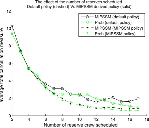
The effect of the number of reserves scheduled Default policy (dashed) Vs MIPSSM derived policy (solid)
MIPSSM (default policy) Prob (default policy) MIPSSM (MIPSSM policy) Prob (MIPSSM policy)
Fig. 4 The effect of theMIPSSMderived reserve use policy
under the graph approach lead to average cancellation measures similar to those from the MiniMax2modification but without the fluctuations. TheUSRapproach lead to the highest average cancellation measures when 10 or fewer reserve crew are available for scheduling. For more than 10 reserve crew thezer osapproach gave the highest cancellation measures.
The difference between the various solution approaches is clearest when there are around 10 to 12 reserve crew available for scheduling, which also appears to be the most sensible number of reserve crew to schedule (due to diminishing returns). In this range, Figure3shows that the best performing solution approach was theSSH. 10 to 12 reserve crew for the given problem instance is approximately proportionate to the number of reserve crew scheduled in reality.
Figure4shows the effect of using theMIPSSMderived reserve use policy described in Sect.7compared to the default policy of using reserve crew as demand occurs. Using the MIPSSMderived policy had the effect of reducing the average cancellation measure.
9.3 Other performance measures and solution reliability
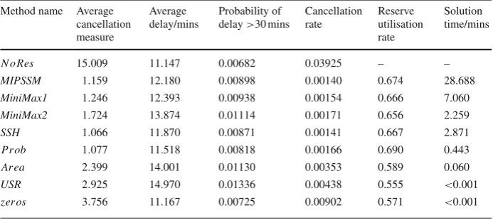
[image:21.439.94.347.56.272.2]The results show that on average theMIPSSMperforms best on cancellation rate, however theMIPSSMis also the slowest method with average solution times of 28 min. The average cancellation measure can be interpreted as the number of cancellations expected in each of the simulations, but this also includes delays which have been converted to a cancellation measure using Eq.1of Sect.2.2. On the whole, theSSHis a highly efficient approach with the lowest cancellation measure, a low average delay and a low solution time in comparison with theMIPSSMapproach. The low solution time of theSSHin comparison to the that of the MIPSSMis a result of the termination criteria being satisfied before more than 10 disruption scenarios are added to the master problem. This result suggests that theSSHoutperforms the MIPSSMapproach because it is possible to find a better reserve crew schedule with fewer input disruption scenarios, provided that some effort is made to find such a set of scenarios. ThePr obapproach has the second lowest average cancellation measure, good average delay performance and a solution time much quicker than those of theMIPSSMbased approaches. The results in Table5suggest that there is merit in both the probabilistic andMIPSSM based approaches (SSHin particular) for scheduling airline reserve crew under uncertainty. Table5also includes performance measures when no reserve crew are scheduled at all as a point of reference. Contrary to expectation the probability of delay over 30 min is lower without reserve crew, as is the average delay, however this can be attributed to the high cancellation rate, since cancelled flights do not count as delays and also to delays introduced when waiting for reserve crew to cover for absent crew.
Figure5shows the spread of cancellation measures corresponding to each method over the 20 repetitions of each method, with each being tested in 20,000 repeat validation simulations. The percentile axis has an exponential scale (cubed) for clarity, as this increases the linearity of the data. Figure5also displays the 100t h percentile (worst case) cancellation measure from each approach, and this is the most appropriate validation criteria for theMiniMax2 objective. TheMiniMax2objective does not have the lowest cancellation measure for the 100t h percentile, so it appears that this objective does not achieve its goal. The reason for this is thatMiniMax2schedules reserve crew with respect to the worst case scenarios in a limited set of scenarios, so when a worst case scenario occurs in the validation simulation which is different from the worst case scenarios used to derive the reserve crew schedule, the reserve crew schedule performs worse than a reserve crew schedule aimed at the average case scenario.
Figure5demonstrates that for each given percentile the ordering of the methods supports the results given in Table5except for thezer osapproach which has the lowest worst case cancellation measure. This result suggests that the worst scenario is, for a very large number of crew to be absent at the start of each day, which is precisely the situation thezer os approach can cope with. TheMiniMax2approach will only achieve it’s goal if such worst case scenarios happen to be in the limited sets of scenarios. The other methods have relatively high worst case cancellation measures because they are aimed at the average case scenario.
Table5and Fig.5show that theMiniMax1andMiniMax2approaches which were aimed at minimising the effects of the worst case scenarios do not appear to have been effective in achieving this goal when considering the relatively high probabilities of delay over 30 min (Table5) and the 100t h percentile (worst case) cancellation measures (Fig.5) associated with these approaches. The possible explanation is that the best reserve crew schedule for one worst case is not the best reserve crew schedule for a different worst case scenario.
0 1 2 3 4 5 6 7 8 9 10 x 105 0
5 10 15 20 25 30 35 40 45
Cancellation measure percentiles from 200000 repeat simulations using an exponentially scaled x−axis
percentile3
Cancellation measure
MIPSSM MiniMax 1 MiniMax 2 SSH Prob Area USR Zeros
60% 70% 80% 90%
MIPSSM Prob Zeros MiniMax1 SSH MiniMax2 Area USR
Fig. 5 Percentile cancellation measures
MIPSSM MiniMax1 MiniMax2 SSH Prob 1
1.5 2 2.5 3 3.5
Solution stability of MIPSSM based methods compared to the probabilistic model
Methods
Average cancellation measure
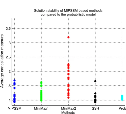
Fig. 6 Solution reliability ofMIPSSMbased methods compared toProb
[image:23.439.93.349.55.322.2] [image:23.439.92.348.329.561.2]method. For this reason further research was performed to investigate the scenario selection mechanism.
10 The effect of scenario sets on reserve crew schedule quality
The basicMIPSSM formulation requires a set of input disruption scenarios. This section attempts to address the issue of solution reliability illustrated in Fig. 6, through careful selection of the scenarios added to theMIPSSMformulation of Sect.5.1. Disruption scenarios were generated randomly in the previous sections. In the case of theSSH, scenarios are selected if the cancellation measure for the new scenario is worse than the cancellation measure in any of the already selected scenarios, with the incumbent reserve crew schedule. This section investigates what makes a good set of scenarios. To answer this question attributes of sets of scenarios are defined. These are defined by the pool of scenarios that scenarios in the set belongs to and the number of scenarios in the set. Three pools of scenarios are considered, and these are generated using the procedure outlined in Fig.7of Sect.10.1. The presence or lack of correlations between the attributes of sets of scenarios and the resultant reserve crew schedule quality was investigated. Sect.10.1presents an investigation into the effect of the number of scenarios selected and the different types of pools from which they
Pool A. 1000 Randomly generated scenarios
Select 200 sets of scenarios of various sizes without replacement from the given pool
For each set of scenarios, solve MIPSSM to find reserve crew schedule
Pool C. 100 scenarios with the lowest associated average reserve schedule cancellaon measure Pool B. Select the 100
scenarios corresponding to the reserve crew schedules with the lowest 100 average cancellaon measures
Test reserve crew schedules in repeat simulaons to derive an associated average cancellaon measure
Plot data point corresponding to a reserve schedule obtained by solving a set of scenarios from a given pool (pool, number of scenarios, average cancellaon measure) Solve MIPSSM for each
single scenario alone
For each set of scenarios from pool A, compute the average cancellaon measure for each scenario over the reserve schedules they were used to generate
Test the 1000 reserve crew schedules in repeat simulaons to derive an associated average cancellaon measure
START
FINISH
[image:24.439.78.363.293.601.2]are selected of scenarios on the quality of reserve crew schedules derived from those sets of scenarios using theMIPSSMformulation.
10.1 Attributes of sets of scenarios
As previously mentioned, the attributes of a set of scenarios are defined as the number of scenarios and the pool from which the scenarios are selected. Each pool of scenarios has a defining criterion for accepting scenarios into the pool.
10.1.1 Pool A: 1000 random scenarios
Pool A consists of 1000 randomly generated scenarios.
10.1.2 Pool B: good individual scenarios
Figure7shows how the two pools of scenarios B and C are derived from pool A. To create pool B, the first step is to solve theMIPSSM formulation for each scenario in pool A on its own to obtain a reserve crew schedule corresponding to each scenario in pool A. Each reserve crew schedule corresponding to each scenario in pool A is then tested in the validation simulation to obtain an associated average cancellation measure. Pool B is then populated with the 100 scenarios from pool A which have the lowest associated average cancellation measures. Pool B represents scenarios, that when solved alone in theMIPSSMformulation, give good reserve crew schedules.
10.1.3 Pool C: good scenarios for sets
To create pool C, 200 sets of scenarios of various sizes are randomly sampled from pool A and solved in theMIPSSMformulation. The reserve crew schedules corresponding to each set of scenarios are tested in the validation simulation to obtain associated average cancellation measures. Pool C is then populated with the 100 scenarios from pool A with the lowest average cancellation measures, where the average cancellation measure is calculated from the cancellation measures corresponding to the sample sets of scenarios they are a member of. Pool C represents scenarios that improve the quality of reserve crew schedules when added to a set of scenarios to be solved in theMIPSSMformulation. Figure7outlines the process of populating pools B and C from pool A. Figure7also illustrates the process of deriving data points for Fig.8, which is designed to show the quality and variance of the quality of reserve crew schedules derived from sets of scenarios selected from each pool of scenarios.
10.2 Testing pools of scenarios
5 10 15 20 25 30 35 40 45 0.8
1 1.2 1.4 1.6 1.8 2 2.2 2.4 2.6
Number of scenarios in a set
Cancellation measure
The effects of the number of scenarios in a set and the type of scenario pool on the resultant solution quality when MIPSSM is solved for the given set
Y= −0.0049X+1.3165 Y= −0.0017X+1.0764 Y= −0.0066X+1.1946 R= −0.2139 R= −0.2155 R= −0.5120 Pool A Pool B Pool C
pool A (1000 random scenarios) pool B (top 100 individual scenarios) pool C (top 100 set scenarios)
Fig. 8 The effect of the pool from which scenarios are selected and the number of scenarios selected on average cancellation measure associated with the reserve crew schedule derived from the given set of scenarios
measure associated with the reserve crew schedule derived from that set of scenarios for all pools. I.e. Increasing the number of scenarios will decrease cancellations/delays. Figure8 also shows that the quality of reserve crew schedules derived from sets of scenarios selected from pools B and C is on average greater than reserve crew schedules derived from sets of scenarios from pool A. Furthermore the quality of reserve crew schedules corresponding to sets of scenarios derived from Pool B is much less sensitive to the number of scenarios in those sets. This is intuitive as scenario pool B consists of scenarios that give good solution quality when solved alone. This also suggests that scenarios that work well as the single input for MIPSSMdo not necessarily lead to improved solutions when used together as a set of input scenarios for theMIPSSM. Figure8shows that the average cancellation measure of reserve crew schedules derived from sets of scenarios selected from pool C has the most convincing negative correlation (highest negative gradient and magnitude of correlation coefficient R) with the number of scenarios in those sets. This is also intuitive as pool C represents scenarios that improve reserve crew schedule when included in a set of scenarios.
The conclusion is that scenarios which are used as input for theMIPSSMcan be divided according to whether they work best as the sole input scenario (pool B) or whether they are scenarios that complement a pre-existing set of scenarios (pool C). The difference in the gradients of the regression lines corresponding to pools B and C in Fig.8shows that pools B and C contain different scenarios. It is also interesting to note that the best result in Fig.8occurred for a set of scenarios derived from pool C that only contained 16 scenarios. Increasing the number of scenarios beyond around 15 leads to an improvement in solution reliability for sets selected from pools B and C, however the same does not occur for the random scenarios of pool A. This is a positive result as solution reliability is one of the MIPSSM’s biggest problems (Fig.6).
[image:26.439.93.350.57.272.2]