1
How Should We Estimate Value-Relevance Models?
Insights from European Data
Enrico Onali
a,+, Gianluca Ginesti
b, Chrysovalantis Vasilakis
ca
Aston Business School, Aston University, Birmingham, England, UK, Post code: B4 7ET. b
Department of Economics, Management and Institutions, University of Naples “Federico II”, Monte S. Angelo University Campus, via Cinthia, 80126, Naples (Italy).
c Bangor Business school and IRES, Universite Catholique de Louvain.
+
Corresponding author: [email protected]; Tel: +44(0)121 204 3060.
© 2017, Elsevier. Licensed under the Creative Commons Attribution-NonCommercial-NoDerivatives 4.0 International http://creativecommons.org/licenses/by-nc-nd/4.0/
Abstract
We study the consequences of unobserved heterogeneity when employing different econometric methods in the estimation of two major value-relevance models: the Price Regression Model (PRM) and the Return Regression Model (RRM). Leveraging a large panel data set of European listed companies, we first demonstrate that robust Hausman tests and Breusch-Pagan Lagrange Multiplier tests are of fundamental importance to choose correctly among a fixed-effects model, a random-effects model, or a pooled OLS model. Second, we provide evidence that replacing firm fixed-random-effects with country and industry fixed-effects can lead to large differences in the magnitude of the key coefficients, with serious consequences for the interpretation of the effect of changes in earnings and book values per share on firm value. Finally, we offer recommendations to applied researchers aiming to improve the robustness of their econometric strategy.
2
How Should We Estimate Value-Relevance Models?
Insights from European Data
Abstract
We study the consequences of unobserved heterogeneity when employing different econometric methods in the estimation of two major value-relevance models: the Price Regression Model (PRM) and the Return Regression Model (RRM). Leveraging a large panel data set of European listed companies, we first demonstrate that robust Hausman tests and Breusch-Pagan Lagrange Multiplier tests are of fundamental importance to choose correctly among a fixed-effects model, a random-effects model, or a pooled OLS model. Second, we provide evidence that replacing firm fixed-random-effects with country and industry fixed-effects can lead to large differences in the magnitude of the key coefficients, with serious consequences for the interpretation of the effect of changes in earnings and book values per share on firm value. Finally, we offer recommendations to applied researchers aiming to improve the robustness of their econometric strategy.
3 1. Introduction
We investigate whether unobserved heterogeneity can lead to misspecifications in the estimation
of value-relevance models. This is an important topic in other related fields such as asset pricing and
corporate finance, as recently documented by Gormley and Matsa (2014). However, the
value-relevance accounting literature has hitherto only partially investigated this issue.
Value-relevance studies aim to assess the extent to which accounting data reflect information that
is “relevant” for firm value as represented by the stock price (Holthausen and Watts, 2001). Over the
last decades, a substantial amount of accounting studies have focused on the value relevance effects
around the implementation of International Financial Reporting Standards, henceforth IFRS (Callao et
al., 2007; Zeff, 2007; Aharony et al., 2010; Devalle et al., 2010; Horton and Serafeim, 2010; Barth et
al., 2012; Tsalavoutas et al., 2012; Barth et al., 2014; Christensen et al., 2015).
The motivation of our study lies in the heterogeneity of the approaches employed in the empirical
literature, which hinders the comparability of findings for different countries (ICAEW, 2014). To
address this issue and to answer calls for more robust econometric analysis in accounting research
(Brüggemann et al, 2013), we investigate the impact of using different approaches on the magnitude
and statistical significance of the coefficients of regression models typically employed in value
relevance studies.
The validity of the coefficient estimates of relevance models is a key topic in the
value-relevance literature (Kothari and Zimmerman, 1995; Barth and Kallapur, 1996; Aboody et al., 2002).
However, the existing literature does not provide clear guidelines to applied researchers on how to
choose among different types of econometric approaches. It is also unclear whether choosing an
inappropriate model may lead to wrong inferences with respect to whether a certain accounting
variable is value relevant or not. This is the focus of our study.
Our contribution to the literature is threefold. First, we demonstrate the importance of employing
4 2010) to decide whether a Fixed Effects (FE) model or a Random Effects (RE) model should be used.
While some papers have used the Hausman test to select the correct model between FE and RE model
(for example, Worthington and West, 2004), they tend not to use the “robust” Hausman test, and in
most cases (for example, Devalle et al., 2010) neither version of the Hausman test is employed. For
cases where the RE model is valid, we point out that the Breusch-Pagan Lagrange Multiplier (LM)
test should be run to choose between the OLS model and the RE model. Using these tests is important
to ensure that the estimator chosen is consistent and efficient. In particular, choosing the FE model
when the RE model should be preferred may lead to insignificant coefficients, because the RE model
is more efficient than the FE model. This is a crucial issue for researchers interested in value
relevance analysis because an insignificant coefficient indicates that a variable is not value relevant.
Second, we investigate the differential impact of firm FE, year FE, country FE, and industry FE.
A recent study by Amir et al. (2016) points out that many empirical accounting researchers tend to
(incorrectly) replace firm FE with other forms of FE, in particular industry FE. Amir et al. (2016)
address this issue only for U.S. listed firms (which prepare their financial statements according to the
U.S. GAAP), and they do not focus on value relevance models. We extend their findings in three
ways: i) we examine value relevance models; ii) we use data for European listed firms for the period
of compulsory IFRS adoption (2005 onwards); and iii) we examine the impact of the length of the
sample period on the bias resulting from neglecting firm FE using Monte Carlo simulations.
Third, we examine whether using different levels of clustering the standard errors leads to
substantially different results, and we check for the potential impact of attrition. We provide evidence
that clustering the standard errors matters, and we emphasise the impact of using a small number of
clusters on the extent of the bias. Attrition bias may also affect the coefficient estimates and overall
explanatory power of the model, and this problem is likely to be more acute for sample periods
5 The structure of the rest of the paper is as follows. Section 2 describes the sample composition
and data. Section 3 examines the impact of model specification on a sample of European listed firms.
Section 4 concludes the paper and offers recommendations for future research.
2. Sample and data
For our empirical analysis, we focus on two models widely employed in the value relevance
literature: the Price Regression Model (PRM) and the Return Regression Model (RRM). These
models constitute the basis to examine the value relevance of book value of equity and earnings, as
well as specific items of financial statements, such as research and development expenditure (Aboody
and Lev, 1998; Kallapur and Kwan, 2004).1
The PRM involves estimating a regression of stock price (P) on book value (BVPS) and earnings
(EPS) per share (Barth et al., 2008):2
Pit = a + bBVPSit + cEPSit + eit (Eq. 1)
where i = 1, 2, …, N represent firms, t = 1, 2, …, T represent years.
The RRM is based on a regression of stock returns on earnings per share and changes in earnings
per share: it it it it it
it
a
bEPS
P
c
EPS
P
e
RET
/
1
/
1
(Eq. 2)where 1 1 it it it it it P P DPS P
RET and ΔEPSit = EPSit – EPSit–1(Barth and Clinch, 2009).
1 These models have also been the focus of similar papers that have examined methodological issues in value
relevance models, such as Barth and Clinch (2009), who evaluate the possibility of omitted variables bias in the PRM and RRM, and the importance of scale effects.
2 We focus on this model, which is based on per-share values, because it is less likely to be prone to scale effects
6 Where P is the stock price as at six months after fiscal year-end (Lang et al., 2006; Barth et al.,
2008) and DPS denotes dividends per share. For simplicity, in the discussion below we use the
notation DEPS = (EPSit /Pit–1) and ΔDEPS = (ΔEPSit /Pit–1). All variables are winsorised at the 1st and
99th percentile to reduce the potential impact of outliers.
We collect accounting data for sample of European listed companies from Amadeus for 71
industries,3 selected on the basis of the first two digits of the U.S. SIC code,4 and 17 European
countries. Price data are collected from Datastream. We choose to examine European listed firms
because the majority of the recent value-relevance studies have focused on Europe, especially to
assess the impact of IFRS reporting on value relevance (Devalle et al., 2010; Barth et al., 2014). The
cross-country nature of our sample enables us test the robustness of our analysis across different
institutional, regulatory and cultural settings (McLeay and Jafaar, 2007; Christensen et al., 2013a,
2013b; Veith and Werner, 2014).
We choose 2005 as the beginning of our sample period because prior to 2005 even listed firms
could use domestic GAAP and this may produce some noise in the data. We choose 2013 as final year
because most of the papers on IFRS focus on sample periods shorter than ten years.
Our initial sample consists of 5,164 companies. To eliminate inconsistencies due to different
reporting dates, we consider only firms with fiscal year-end as of December 31st. This selection
criterion results in 1,208 companies leaving the sample. We also exclude companies with a negative
book value (15 companies). Data availability for our main variables of interest, P, BVPS, and EPS,
during the sample period 2005-2013 results in 2,860 companies selected.For the RRM, for which we
need data also on DPS and the first lag of P, we have 2,459 companies. In Appendix A we report the
composition of our sample and the mean of each variables.
3 The initial number of industries in the sample is 73. For two of these industries, data availability for the
variables employed in the regressions results in zero observations in the regressions. Therefore, effectively we have 71 industry clusters.
4The two-digit SIC code is commonly employed in accounting research to identify industry clusters (see,
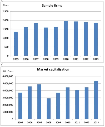
7 As shown in Figure 1, the sample is unbalanced, with firms exiting and entering the sample over
time, causing drastic changes in market capitalization and sample size. The most dramatic change
seems to be in conjunction with the financial crisis (2008-2009). We therefore have an unbalanced
panel data set, and attrition bias (Hausman and Wise, 1979) may be present. We address this issue in
sections 3.3 and 3.4.
[Insert Figure 1 Here]
3. Empirical examination of model specification
3.1. Choosing among OLS, RE models and FE models
We start our empirical examination by offering evidence on the importance of two tests: the
Hausman test, which is employed to choose between the FE and the RE model; and the
Breusch-Pagan LM test, which indicates whether a researcher should use the RE model or the OLS model.
We argue that selecting the wrong econometric model is a serious problem because it can lead to
wrong inferences. For example, choosing the RE model when the FE model should be preferred
(because the Hausman test is significant) may lead to wrong coefficient estimates. This bias may
significantly affect the magnitude (and, potentially, sign) of the coefficients for the PRM or RRM
model. On the other hand, if the Hausman test is insignificant the RE model should be chosen, and
using the FE model may result in statistically insignificant coefficients even when they would be
statistically significant for the RE model. Similarly, if the Breusch-Pagan LM test is significant, the
RE model should be preferred. However, if the Breusch-Pagan LM test is insignificant, the pooled
OLS model will be more efficient than the RE model.
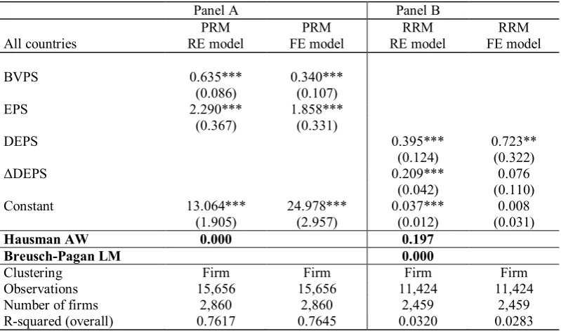
In Table 1 we report the results of estimating the PRM and RRM on the whole sample, and we
employ the “robust” Hausman test (Arellano, 1993, and Wooldridge, 2002, and 2010) and the
Breusch-Pagan LM test to understand which model should be employed. Table 1 shows that using the
RE model for the PRM leads to inconsistent coefficient estimates, because the Hausman p-value is
8 the RE and FE models, suggesting that the RE model leads to inconsistent estimates. Conversely,
using the FE model for the RRM leads to an insignificant coefficient for ΔDEPS (see table in Table 1,
Panel B), while using the RE model results in significant coefficients for both ΔDEPS and DEPS. This
is consistent with the higher efficiency for the RE estimator relative to the FE estimator. Note that, as
evidenced by the Hausman p-value (0.197), the RE model should be preferred to the FE model. The
Breusch-Pagan LM test results for Panel B suggest that the RE model should be preferred to the OLS
model, because the P-value is less than 0.05.
[Insert Table 1 Here]
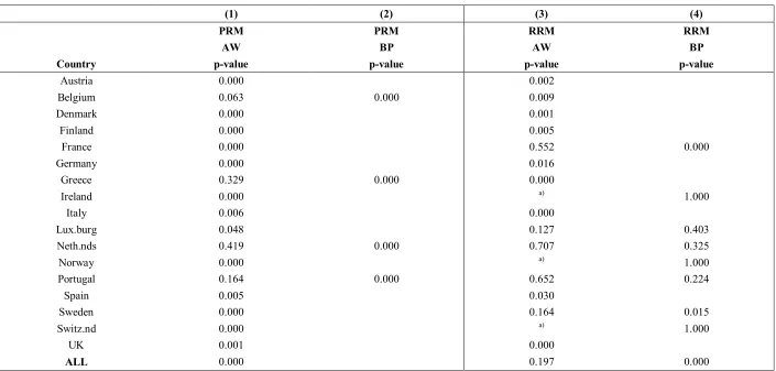
In Table 2 we provide the results of robust Hausman tests and Breusch-Pagan LM tests for
country-based sub-samples. In Table 2 we denote the robust version of the Hausman test AW, the
Breusch-Pagan LM test BP.5 This table is connected with Tables 3 and 4 (reported below), and in
particular specification (3), which includes firm FE, and specification (1), which considers a pooled
OLS without any FE.
The results reported in Table 2 show that in 13 out of 17 cases for the PRM we reject the null
hypothesis that the RE model is consistent, and we find evidence that the FE model is the most
suitable method for the estimation of the PRM. For certain countries (for example, Portugal), lack of
significance for the Hausman test may be due to the small number of observations, which may reduce
the power of the test (Clark and Linzer, 2015). Conversely, the model with firm FE does not perform
very well for the RRM: only for 9 out of 17 countries is the model with firm FE preferred to the RE
model. The RE model is preferred for countries with a large number of observations (such as France),
and even for the whole sample considering all 17 countries. This finding suggests that, in this case,
the number of observations is unlikely to be the main cause for lack of significance of the Hausman
test. Further, the results for the Breusch-Pagan LM test suggest that in six out of the nine cases (the
eight cases for the individual countries and the case for the whole sample) the pooled OLS should be
5 Using the original version of the Hausman test also results in similar rejection rates. However, the results for
9 the preferred model (in other words, the FE model and the RE model do not perform better than the
pooled OLS model). Some of these cases refer to countries with a small number of observations (for
example, Luxembourg or Ireland).
[Insert Table 2 Here]
3.2. Results for country-based sub-samples: coefficient estimates and statistical significance
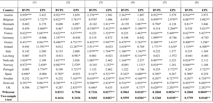
In Tables 3 and 4 we report the results (coefficient estimates and statistical significance level) for
six different specifications for the PRM and the RRM, respectively, for 17 regressions (one for each
country in the sample):6
i) Pooled OLS with heteroskedasticity-robust standard errors, clustered on the firm level (model 1);
ii) Pooled OLS with year FE, and heteroskedasticity-robust standard errors, clustered on the firm level (model 2);
iii) FE model (where the panel unit is the firm), with heteroskedasticity-robust standard errors, clustered on the firm level (model 3);
iv) FE model (where the panel unit is the firm) with year FE, and with heteroskedasticity-robust standard errors, clustered on the firm level (model 4);
v) Pooled OLS with industry FE, and heteroskedasticity-robust standard errors, clustered on the firm level (model 5);
vi) Pooled OLS with industry and year FE, and heteroskedasticity-robust standard errors, clustered on the firm level (model 6).7
6 We decide to cluster the standard errors on the firm level because the number of industries is less than 20 for
six countries, and papers such as Cameron and Miller (2015), Carter et al. (2013), Kezdi (2004), and Wooldridge (2003) warn against clustering the standard errors when the number of clusters is small. In particular, Carter et al. (2013) suggest that even when the actual number of clusters is above 20 the “effective” number of clusters can be smaller once cluster heterogeneity is allowed for. This is likely to be the case in our sample, because the number of observations for each cluster is not fixed (that is, we have unbalanced clusters). For Luxembourg we have a number of firms smaller than 20: this suggests the results for Luxembourg should be read with caution because the standard errors may be biased. For this reason, we run the six regressions for Luxembourg even without clustering. The results for the regressions without clustering (untabulated but available upon request) suggest that clustering in this case generates smaller standard errors.
7 None of the firms in the sample changes industry or country of origin during the sample period. For this
10 The results suggest that the type of specification chosen bears a strong impact on the magnitude
and statistical significance of the coefficients of the variables, and, in some cases, even the sign of the
coefficient changes. For instance, in Table 3 (PRM), we find that for several countries (Denmark,
Finland, Luxembourg and Norway), when we introduce both firm FE and year FE the sign coefficient
of BVPS changes from positive (pooled OLS case) to negative. For some countries (e.g. Germany),
the introduction of firm FE and year FE causes a dramatic reduction in the size and statistical
significance of the coefficient on BVPS (from 1.183, significant at the 1% level) to 0.108
(insignificant).
Wilcoxon and two-sample t-tests (reported at the bottom of Table 3) suggest that adding firm FE,
country FE, or industry FE leads to significantly different coefficients for EPS, but not for BVPS.
Adding only year FE does not lead to significantly different coefficients in comparison with the
pooled OLS model. The coefficient on BVPS is significant at the 5% level only in eight cases out of
17 for specifications (1), (2), and (3), in nine cases for specification (4) and in ten cases for
specifications (5) and (6).
The coefficient on EPS is significant in seven cases of out 17 for specification (5), in eight cases
for specification (6), and in nine cases for specifications (1) – (4). In other words, the specification
chosen affects inferences on whether BVPS or EPS bear an impact on stock price.
[Insert Table 3 Here]
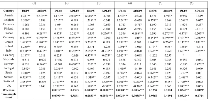
Consistent with the results reported in Table 3, Table 4 highlights that there are substantial
changes for the slope coefficients and related statistical significance of both of the variables of the
RRM when firm FE or industry FE are included. The average coefficient on DEPS tends to increase
as a result of the inclusion of firm FE from 0.85 to 1.83 (this difference is significant, according to
both Wilcoxon tests and two-sample t-tests), while the coefficients on ΔDEPS tend to decrease (the
mean drops from 0.34 to -0.36, and the Wilcoxon and two-sample t-tests are significant at the 1%
level). The coefficient for ΔDEPS in the models with firm FE (and even in the model with both
11 stock returns).8 This result is not due to an outlier that is pushing the average coefficient for ΔDEPS
below zero (as said above, we winsorise all variables).9
When industry FE (but not year FE) are in the regressions, the results are similar to those for the
model without year FE, firm FE or industry FE (pooled OLS), and also to those of the specification
with only year FE. However, when both industry FE and year FE are considered, the results are
similar to those with both firm FE and year FE. As for the statistical significance of the models, the
results for the coefficients on DEPS are significant in 11 cases out of 17 for specifications (1), (3), and
(4), in nine cases for specification (2), and in eight cases for specifications (5) and (6). For ΔDEPS,
there are only six significant cases for specifications (1) and (2), and including firm FE reduces
further the number of significant coefficients (four when only firm FE are included, in model (3), and
two if both firm and year FE are included, in model (4)). For models (5) and (6) there are three and
five significant coefficients, respectively.
[Insert Table 4 Here]
In Tables 3 and 4 we have clustered the standard errors on the firm level. Because of the
importance of clustering the standard errors (Petersen, 2009), we now briefly examine the impact of
running the same regressions without clustering. These results are untabulated but available from the
authors upon request. As reported above, for Luxembourg the number of firm-clusters is relatively
small and this may have led to biased standard errors (Cameron and Miller, 2015). However, when we
estimate the regressions without clustering on the firm level, the results in terms of statistical
significance of the coefficients on BVPS and EPS remain unaltered relative to those reported in Table
3. The results related to Table 4, instead, change in a number of cases. The number of significant
8 The high proportion of negative coefficients for ΔDEPS decreases substantially when we employ Earnings
Before Interest and Taxes (EBIT), instead of earnings. This suggests that the transitory earnings issue (Ota, 2003) may be causing such counterintuitive results.
9 For the specification with only year FE, the coefficient on ΔDEPS is positive in 15 cases out of 17, while in the
12 coefficients on DEPS increases when there is no clustering for all six specifications,10 suggesting that
neglecting within-firm correlation may lead to upward biased standard errors. However, this is not the
case for the coefficients on ΔDEPS, for which the number of significant coefficients decreases,
increases, or remains the same.11
We now examine briefly the results reported in Tables 3 and 4 in conjunction with the results
reported in Table 2. For the sake of brevity, we focus on several cases that stand out. For example, for
Italy the results for the PRM coefficients are significant only when firm FE are included
(specifications (3) and (4) in Table 3). The results in Table 2 for the robust version of the Hausman
test confirm that firm FE matter: the p-value for Italy for the PRM is 0.006. Similarly, the results in
Table 4 for Austria suggest that the coefficient on ΔDEPS is positive and significant when firm FE are
not included (columns (1) and (2) of Table 4) and negative and insignificant when firm FE are
included. The p-value for the robust version of the Hausman test is 0.002, confirming that including
firm FE has a significant impact on the coefficient estimates, and the RE and OLS coefficient
estimates are therefore inconsistent.
3.3 The role of different types of fixed effects and attrition
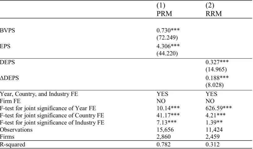
In Table 5, we report the results of OLS regressions for the PRM and RRM where year FE,
country FE, and industry FE are included, while firm FE are excluded. We also report F-tests to show
the incremental explanatory power of each type of FE. This is useful to examine whether a type of FE
is redundant once the other types of FE are included. All types of FE are important, as the F-tests are
significant at either the 1% or 5% level. This finding suggests that time-varying (but panel-invariant)
variables captured by year effects, industry time-invariant variables, and country time-invariant
variables are, at least to some extent, independent of each other.
10 The number of significant coefficients on DEPS increases when clustering is not performed, as follows: from
11 to 13 for specification (1), from nine to 13 for specification (2), from 11 to 12 for specifications (3) and (4), from eight to 12 for specification (5) and from eight to ten for specification (6).
11 The number of significant coefficients on ΔDEPS increases when clustering is not performed for
13 [Insert Table 5 Here]
In Tables 6 and 7 we dig deeper into the impact of unobserved heterogeneity by comparing the
results for a pooled OLS model with those of models that allow for a variety of FE: i) pooled OLS; ii)
year FE; iii) firm FE; iv) both firm and year FE; v) industry FE; vi) industry and year FE; and vii)
country and year FE.12
Finally, to examine the potential impact of attrition, we also run the regressions with firm and
year FE with a balanced panel of 528 firms that are in our sample throughout the period from 2005 to
2013 (model (8)). The remaining firms come from 15 countries (we lose Luxembourg and Denmark)
and 56 industries.
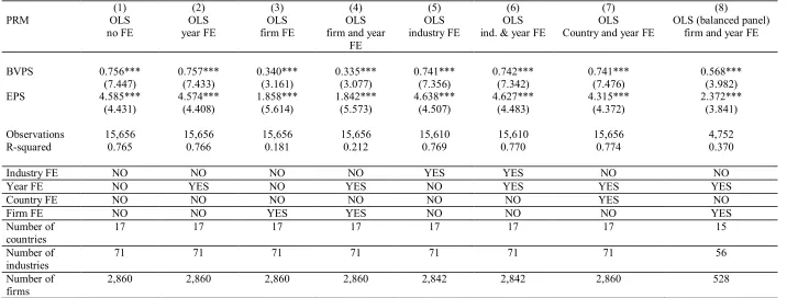
Consistent with the results reported above for the 17 country sub-samples (Table 3), the results
reported in Table 6 demonstrate that adding firm FE reduces the coefficient on EPS (from around 4.5
to around 1.8) in the PRM. The coefficient on BVPS in the PRM also decreases (from around 0.76 to
around 0.34). Industry FE, country FE and year FE bear a negligible effect on either coefficient.
According to Amir et al. (2016), as the number of industries increases, the importance of industry FE
should increase. However, despite the fact that we have 71 industry clusters but only 17 country
clusters, industry FE are not more important than country FE. This finding suggests that heterogeneity
at the industry level for European studies is not very strong. Only firm FE result in a substantial
decrease in the coefficients on both BVPS and EPS, which remain statistically significant for all
specifications. Firm FE also result in a substantial decrease in R-squared values. In specification (8),
where we use a balanced panel of 528 firms for a model with both firm FE and year FE, the
explanatory power of the model increases relative to the corresponding specification with an
12 In untabulated results, we also look at the impact of country-level institutional factors such as: Rule of law,
14 unbalanced panel: the R-squared increases from 21.2% to 37%.13 This finding indicates that the
association between market and book values for new firms and firms that eventually become delisted
is weaker than for other firms, which in turn may indicate attrition bias, which is particularly harmful
for FE models (Verbeek, 1990).
[Insert Table 6 Here]
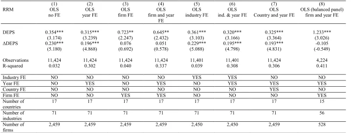
The results in Table 7 confirm the results reported in Table 4 with respect to the impact of firm
FE on the coefficients of both DEPS and ΔDEPS: firm FE result in an increase of the coefficient on
DEPS and a decrease in the coefficient on ΔDEPS. Unlike in the sub-sample estimations, the
coefficient on ΔDEPS does not become negative. Industry and country FE do not bear a significant
impact on the coefficient estimates of either variable. The coefficients on DEPS are significant for all
specifications but those on ΔDEPS are insignificant when firm FE are included. The inclusion of year
FE is associated with a strong increase in R-squared values. This finding suggests that the RRM
model is highly sensitive to macroeconomic changes that affect all firms in a certain year. Finally, the
results for the FE model with year FE when we use a balanced panel of 528 firms suggest that the
R-squared improves relative to that of the same regression on an unbalanced panel (from 33.7% to
41.1%). This finding is consistent with the results reported for the PRM in Table 6. The magnitude of
the coefficient on DEPS increases. The coefficient on ΔDEPS remains insignificant, similar to what
reported for the unbalanced panel.14
[Insert Table 7 Here]
3.4 Monte Carlo simulations
The results of our empirical analysis show that replacing firm FE with other types of FE may be
inappropriate, consistent with the findings by Amir et al. (2016), based on Monte Carlo simulations.
Amir et al. (2016), however, focus on a fixed number of periods (10). In this section, we examine the
13 This is the “within” R-squared, based on the variation within firm clusters.
14 In untabulated results, we have run regressions that exclude countries for which the RE model is preferred to
15 impact of the length of the sample period and attrition on the bias resulting from neglecting firm FE.
In particular, we provide an examination of the impact of omitting firm FE when year, country, and
industry FE are included on the bias of the coefficients. We also compare the size of the standard
errors of the coefficients across specifications, to evaluate the relative efficiency of the OLS, RE and
FE model.
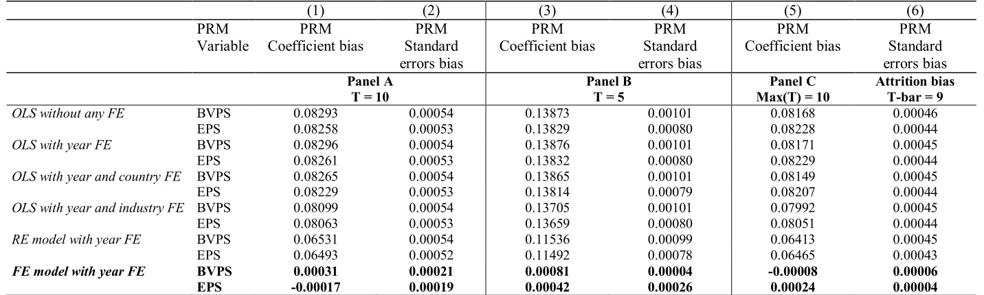
Our Monte Carlo simulations are calibrated according to the parameter values estimated in the
previous section and reported in Table 5.For the sake of brevity, we focus our discussion on the PRM,
but our results extend to the RRM as well.
The specifications considered are as follows: i) pooled OLS; ii) OLS with year FE; iii) OLS with
year and country FE; iv) OLS with year and industry FE; v) RE model with year FE; and vi) FE
model (that is, model with firm FE) with year FE.
We run 500 replications using simulated data for a sample of firms with the same composition (in
terms of country and industry of origin of the firms) as that used for the empirical analysis above. This
is done by replacing the data for P, BVPS and EPS for each firm in the dataset with simulated data.
For the simulations, we keep in our dataset only firms for which we have information about the
country and SIC code. The number of firms is therefore 2,842, as in Table 6, (models (5) and (6)). To
understand how the length of the sample period affects the bias in the coefficients and standard errors,
we run the replications considering 10 periods for Panel A and 5 periods for Panel B (that is, T = 10
in the first case, and T = 5 in the second case). Moreover, to examine the effect of attrition bias, Panel
C considers a maximum number of periods equal to 10 (Max(T) = 10), but with attrition bias leading
to an average time span equal to 9 periods (T-bar = 9).15 More details on the Data Generating Process
(DGP) are presented in the notes below Table 8.
In both cases (T = 10, and T = 5), the models with the firm and year FE provide the smallest bias
in both the coefficients and standard errors of the coefficients. The results show that the average
15 As explained in the notes to Table 8, we allow 20% of the firms to exit the sample from the sixth period
16 coefficient bias increases as T decreases when firm FE are not included. For Panel C, we find that the
bias is slightly bigger than for T = 10, but smaller than for T = 5, consistent with the fact that T-bar =
9. The bias is larger for OLS models, and slightly smaller for the RE model. However, in both cases
the bias is substantial. Even the bias for the standard errors is smallest for the FE model with year FE.
These findings suggest that the impact of neglecting firm FE becomes bigger as T decreases, and
attrition bias exacerbates this problem.
[Insert Table 8 here]
4. Conclusions and implications for future research
In this study, we have investigated whether unobserved heterogeneity is important in
value-relevance research as it is in other areas of the economics and finance literature.
We have used a large panel of European listed firms to investigate the impact of firm FE, industry
FE, and country FE on the coefficient estimates and corresponding t-statistics and p-values. While
most empirical studies on value relevance focus their discussion on the estimated t-statistics and
p-values, wrong coefficient estimates can seriously impair the validity of the economic interpretation of
valuation models. For example, in the PRM, the coefficient on EPS represents the change in stock
price following a change by one unit in EPS. Therefore, a biased regression coefficient can lead
researchers to over- or under-estimate the importance of changes in EPS when assessing the value of a
company. This problem is also likely to undermine the reliability of empirical studies evaluating the
effects of the changes in accounting regulation on capital markets, leading to important implications
for policy making. A positive and statistically significant coefficient is not enough to evaluate the
impact of a regulation, because policy makers are often interested in the change in the magnitude of
the coefficient. For example, an increase in the coefficient on EPS in the post-IFRS period may be
interpreted as an indication of stronger value relevance of EPS (Devalle et al., 2010).
In this paper, we have offered several important contributions. First, we have uncovered important
17 models are employed separately for each of the country-based sub-samples. Industry FE, on the other
hand, do not appear to bear a substantial impact on inferences, despite the fact that the number of
industry dummies in our sample is rather large (71). In particular, we show that neglecting firm FE in
the estimation of the PRM and RRM may lead to a substantial bias in both the size of the coefficients
and the corresponding t-statistics of the variables of the PRM and RRM. Using Monte Carlo
simulations, we have shown that the bias increases as the sample period becomes shorter, or in the
presence of attrition bias.
Second, our results have demonstrated that both industry FE and country FE bear a negligible
effect on the magnitude and statistical significance of the coefficients. For this reason, allowing for
industry FE and country FE may not be enough to correctly estimate the impact of the variables in the
PRM and RRM for studies based on European listed firms.
Finally, we examine the impact of clustering the standard errors and attrition and we find that
both of them can lead to wrong inferences. Clustering the standard errors should allow for the impact
of a small number of cluster on the bias of the standard error estimates. Attrition is particularly
important for studies that consider the period of the financial crisis, because of the large number of
firms that exit the sample during this period.
To decide whether to add or not firm FE in the estimation of the PRM and RRM in a European
setting, we suggest that researchers employ “robust” Hausman tests, because the choice between RE
and FE models is sample-dependent and thus which model should be preferred cannot be determined
a priori. If the RE model is preferred, researchers should also test whether the pooled OLS model
may be appropriate using the Breusch-Pagan LM test. Further, we suggest that year FE be included in
the regression, unless the researcher is interested in the effect of time-varying macroeconomic
components whose coefficients would be unidentified in the presence of year FE. Robustness tests
considering the impact of industry and country FE and clustering the standard errors on different
18 To support researchers interested in value relevance studies in Europe, we also provide a
“toolbox" in Table 9, which summarises the main implications of our findings.
[Insert Table 9 Here]
Clearly, we have not assessed the influence of different estimation techniques on the PRM and
RRM under all conceivable conditions. However, our findings support researchers interested in
evaluating the impact of regulation on value relevance by offering guidance on how different
19 References
Aboody, D., J. Hughes, and J. Liu. 2002. Measuring Value Relevance in a (Possibly) Inefficient Market. Journal of Accounting Research (40): 965-986.
Aharony, J., R. Barniv, and H. Falk. 2010. The Impact of Mandatory IFRS Adoption on Equity Valuation of Accounting Numbers for Security Investors in the EU. European Accounting Review 19 (3): 535-578.
Amir, E., Carabias, J.M., Jona J., and Livne J., 2016. Fixed-Effects in Empirical Accounting Research. Working Paper. http://ssrn.com/abstract=2634089, March.
Arellano, M. 1993. On the testing of correlated effects with panel data. Journal of Econometrics 59 (1-2): 87-97.
Barth, M.E., and S. Kallapur. 1996. The effects of cross-sectional scale differences on regression results in empirical accounting research. Contemporary Accounting Research 13 (2): 527-567.
Barth, M.E., W.R. Landsman, and M.H. Lang. 2008. International Accounting Standards and accounting quality. Journal of Accounting Research 46 (3): 467-498.
Barth, M.E., and G. Clinch. 2009. Scale Effects in Capital Markets-Based Accounting Research. Journal of Business Finance & Accounting 36 (3) & (4): 253-288.
Barth, M.E., W.R. Landsman, M.H. Lang, and C. Williams. 2012. Are IFRS-Based and US GAAP-Based Accounting Amounts Comparable? Journal of Accounting and Economics 54: 68-93.
Barth, M.E., W.R. Landsman, D. Young, and Z. Zhuang. 2014. Relevance of Differences between Net Income based on IFRS and Domestic Standards for European Firms. Journal of Business Finance & Accounting, 41 (3) & (4): 297-327.
Breusch, T.S., and A. R. Pagan. 1980. The Lagrange Multiplier Test and its Applications to Model Specification in Econometrics. Review of Economic Studies 47 (1): 239-253.
Brüggemann, U., J. Hitz, and T. Sellhorn. 2013. Intended and unintended consequences of mandatory IFRS adoption: A review of extant evidence and suggestions for future research. European Accounting Review 22: 1-37.
20 Cameron, A.C., and D. L. Miller. 2015. A Practitioner’s Guide to Cluster-Robust Inference. Journal of Human Resources 50: 317-372.
Carter, A. V., K. T. Schnepel, and D. G. Steigerwald. 2013. Asymptotic Behaviour of a t Test Robust to Cluster Heterogeneity. University of California-Santa Barbara. Unpublished. http://economics.ucdavis.edu/events/papers/Steigerwald56.pdf.
Christensen, H.B., L. Hail, and C. Leuz. 2013a. Mandatory IFRS Reporting and Changes in Enforcement. Journal of Accounting and Economics 56: 147-177.
Christensen, H.B., L. Hail, and C. Leuz. 2013b. Proper Inferences or a Market for Excuses? The Capital-Market Effects of Mandatory IFRS Adoption. Working Paper, University of Chicago and University of Pennsylvania.
Christensen, H.B., E. Lee, M. Walker, and C. Zeng. 2015. Incentives or Standards: What Determines Accounting Quality Changes Around IFRS Adoption? European Accounting Review 21: 31-61.
Clark, T. S., and D. A. Linzer. 2015. Should I Use Fixed or Random Effects? Political Science Research and Methods 3: 399-408.
Devalle, A., E. Onali, and R. Magarini. 2010. Assessing the value relevance of accounting data after the introduction of IFRS in Europe. Journal of International Financial Management & Accounting 21 (2): 85-119.
Gormley, T. A., and D. A. Matsa. 2014. Common Errors: How to (and Not to) Control for Unobserved Heterogeneity. Review of Financial Studies 27 (2): 617-661.
Hausman, J. A., and D. A. Wise. 1979. Attrition Bias in Experimental and Panel Data: The Gary Income Maintenance Experiment. Econometrica 47 (2): 455-473.
Holthausen, R. W., and R. L. Watts. 2001. The relevance of the value-relevance literature for financial accounting standard setting. Journal of Accounting and Economics 31: 3-75.
Horton, J., and G. Serafeim. 2010. Market Reaction to and Valuation of IFRS Reconciliation Adjustments: First evidence from the UK. Review of Accounting Studies 15: 725-751.
ICAEW, 2014. The Effects of Mandatory IFRS Adoption in the EU: A Review of Empirical Research. Institute of Chartered Accountants in England and Wales (ICAEW), October.
21 Kezdi, G. 2004. Robust Standard Error Estimation in Fixed-Effects Panel Models. Hungarian Statistical Review 9: 95-116.
Kothari, S.P., and J. Zimmerman. 1995. Price and Return Models. Journal of Accounting and Economics, 20 (2): 155-92.
Lang, M., J. Raedy, and W. Wilson. 2006. Earnings Management and Cross Listing: Are Reconciled Earnings Comparable to US Earnings. Journal of Accounting and Economics 42: 255-283.
La Porta, R., F. Lopez-de-Silanes, A. Shleifer, and R. Vishny. 1998. Law and finance. Journal of Political Econonomy 106: 1113-1155.
McLeay, S., and A. Jaafar. 2007. Country Effects and Sector Effects on the Harmonization of Accounting Policy Choice. Abacus 23: 156-189.
Nobes, C. (2001). GAAP 2001 – a survey of national accounting rules benchmarked against international accounting standards. International Forum Accounting Development (IFAD).
Petersen, M.A. 2009. Estimating standard errors in finance panel data sets: Comparing approaches. Review of Financial Studies 22 (1): 435-480.
Shalev, R., Zhang, I.X., and Y. Zhang. 2013. CEO Compensation and Fair Value Accounting: Evidence from Purchase Price Allocation. Journal of Accounting Research 51 (4): 819-854.
Tsalavoutas, I., André, P., and L. Evans. 2012. The transition to IFRS and the value relevance of financial statements in Greece. British Accounting Review 44 (4): 262-277.
Veith, S., and J.R. Werner. 2014. Comparative Value Relevance Studies: Country Differences Versus Specification Effects. The International Journal of Accounting 49: 301-330.
Verbeek, M. 1990. On the estimation of a fixed effects model with selectivity bias. Economics Letters, 34, 267-270.
Wooldridge, J. M. 2002. Econometric Analysis of Cross Section and Panel Data. Cambridge, MA: MIT Press.
Wooldridge, J. M. 2003. Cluster-Sample Methods in Applied Econometrics. Papers and Proceedings of the One Hundred Fifteenth Annual Meeting of the American Economic Association, Washington, DC, January. The American Economic Review 93 (2), 133-138.
Wooldridge, J. M. 2010. Econometric Analysis of Cross Section and Panel Data. Cambridge, MA: MIT Press, Second Edition.
23
Table 1: Impact of using incorrectly the FE model or the RE model
.
Panel A Panel B
PRM PRM RRM RRM
All countries RE model FE model RE model FE model
BVPS 0.635*** 0.340***
(0.086) (0.107)
EPS 2.290*** 1.858***
(0.367) (0.331)
DEPS 0.395*** 0.723**
(0.124) (0.322)
ΔDEPS 0.209*** 0.076
(0.042) (0.110) Constant 13.064*** 24.978*** 0.037*** 0.008
(1.905) (2.957) (0.012) (0.031)
Hausman AW 0.000 0.197
Breusch-Pagan LM 0.000
Clustering Firm Firm Firm Firm
Observations 15,656 15,656 11,424 11,424 Number of firms 2,860 2,860 2,459 2,459 R-squared (overall) 0.7617 0.7645 0.0320 0.0283
Notes: The two specifications employed are as follows:
Panel A: PRM: Pit = a + bBVPSit + cEPSit + eit
Where Pit is stock price, as at six months after fiscal year-end (Lang et al., 2006; Barth et al., 2008). BVPSit and EPSit are the book
value per share, and the earnings per share, respectively. All variables are winsorised at the 1st and 99th percentile.
Panel B: RRM:
it it it it
it
it a bEPS P c EPS P e
RET / 1 / 1
where 1 1 it it it it it P P DPS P
RET and ΔEPSit= EPSit – EPSit–1(Barth and Clinch, 2009).
Hausman AW refers to the refinement of Hausman’s test by Arellano (1993) and Wooldridge (2002, 2010) method, which allows for errors that are not Independent and Identically Distributed (IID). Breusch-Pagan LM denotes Breusch-Pagan LM test for the choics of either RE model or Pooled OLS.
24
Table 2: Results for the robust Hausman and Breusch-Pagan LM tests for PRM and RRM for 17 European countries.
(1) (2) (3) (4)
PRM PRM RRM RRM
AW BP AW BP
Country p-value p-value p-value p-value
Austria 0.000 0.002
Belgium 0.063 0.000 0.009
Denmark 0.000 0.001
Finland 0.000 0.005
France 0.000 0.552 0.000
Germany 0.000 0.016
Greece 0.329 0.000 0.000
Ireland 0.000 a) 1.000
Italy 0.006 0.000
Lux.burg 0.048 0.127 0.403
Neth.nds 0.419 0.000 0.707 0.325
Norway 0.000 a) 1.000
Portugal 0.164 0.000 0.652 0.224
Spain 0.005 0.030
Sweden 0.000 0.164 0.015
Switz.nd 0.000 a) 1.000
UK 0.001 0.000
ALL 0.000 0.197 0.000
25
Table 3: Results for the PRM regressions for 17 European countries: estimated coefficients for BVPS and EPS.
(1) (2) (3) (4) (5) (6)
Country BVPS EPS BVPS EPS BVPS EPS BVPS EPS BVPS EPS BVPS EPS
Austria 0.959*** 3.432 0.921*** 3.839 2.376*** 1.941 2.363*** 1.887 0.952*** 3.579 0.916*** 3.973 Belgium 0.824*** 3.722** 0.822*** 3.761** 0.978* 1.086 0.978* 1.141 0.899*** 2.978** 0.887*** 3.082** Denmark 0.602 6.178 0.608 6.097 -0.142 3.411*** -0.159 3.087*** 0.794* 4.128 0.817* 3.846
Finland 0.459 5.604** 0.467 5.538** -0.530*** 5.412*** -0.496** 5.190*** 0.514 5.204** 0.539 5.013** France 0.622*** 5.687*** 0.622*** 5.677*** 0.223 1.525*** 0.225 1.463*** 0.626*** 5.449*** 0.627*** 5.437*** Germany 1.183*** -0.806 1.187*** -0.830 0.119 0.872 0.108 0.842 1.099*** -0.746 1.106*** -0.783
Greece 0.431*** 4.841*** 0.446*** 4.751*** 0.452*** 5.947*** 0.479*** 5.765*** 0.388*** 3.413* 0.408*** 3.296* Ireland 0.945 11.591*** 0.812 12.287*** 3.911*** -0.033 3.634*** 0.769 1.771** 5.610* 1.519** 6.508**
Italy 0.142 2.260 0.153 2.088 1.079*** 1.764*** 1.106*** 1.543** 0.225 1.577 0.235 1.369 Lux.burg 0.007 0.675 -0.011 0.981* 0.003 -0.021 -0.038** 0.316*** 0.021 -1.972 -0.041 -0.401 Neth.nds 1.024*** 2.109 1.037*** 2.026 1.085*** 2.462 1.164*** 2.257 0.807*** 2.223 0.824*** 2.112
Norway 0.872*** 2.658* 0.882*** 2.570* -0.165 1.252** -0.091 1.131* 0.834*** 1.261 0.846*** 1.168 Portugal 0.095 3.774** 0.109 3.721** 1.125 2.062 1.222 1.746 0.255 3.772** 0.247 3.722**
Spain 0.696* -0.004 0.705* -0.033 0.167* 4.521*** 0.162* 4.600*** 0.305* 0.267 0.308* 0.254 Sweden 0.252 7.161*** 0.252 7.165*** 0.610*** 4.210*** 0.617*** 4.168*** 0.287* 6.727*** 0.287* 6.724*** Switz.nd 0.391*** 9.081*** 0.385*** 9.122*** 0.580*** 2.814*** 0.516*** 2.855*** 0.459*** 8.570*** 0.455*** 8.605*** UK 0.304 2.748*** 0.287 2.835*** 0.446* 0.635 0.419* 0.737* 0.620*** 2.203*** 0.602*** 2.282***
Wilcoxon 0.8313 0.7946 0.7226 0.0277** 0.5862 0.0245** 0.2868 0.0036*** 0.2868 0.0049***
Two-sample
t-test 0.4416 0.3436 0.5602 0.0483** 0.5595 0.0384** 0.3268 0.0185** 0.3759 0.0160**
Notes: This table presents the coefficients for the variables of the PRM using a variety of specifications with different types of fixed effects (FE). PRM stands for Price Regression Model. For more information on this model, see notes to Table 1 and equation (1). The six specifications employed are as follows: (1) Pooled OLS, (2) Pooled OLS with year fixed-effects, (3) FE regression (firm fixed-effects), (4) FE regression with year fixed-effects, (5) OLS with industry fixed-effects, (6) OLS with both industry and year fixed effects. For all specifications, standard errors are heteroscedasticity-robust and clustered at the firm level. Wilcoxon denotes the p-value for a Wilcoxon signed-rank test (Wilcoxon, 1945) on the distributions of the coefficients for BVPS and EPS for specification (1) as compared to specifications (2) – (6). The null hypothesis is that both distributions are the same. Two- sample t-test reports the p-value for a test for equality of means of the distribution of the coefficient for specification (1) as compared to specifications (2) – (6).
26
Table 4: Results for the RRM regressions for 17 European countries: estimated coefficients for DEPS and ΔDEPS.
(1) (2) (3) (4) (5) (6)
Country DEPS ΔDEPS DEPS ΔDEPS DEPS ΔDEPS DEPS ΔDEPS DEPS ΔDEPS DEPS ΔDEPS
Austria 1.247** 2.536*** 1.170** 2.008*** 6.009*** -1.306 4.346** -0.598 1.471 1.914* 0.986 1.519 Belgium 0.560** 0.199 0.515** 0.099 1.218*** -0.341 1.224*** -0.429 0.578** 0.164 0.569** 0.027 Denmark 1.261 0.336 1.054 0.264 1.703 -0.660 1.713 -0.717 1.190 0.313 1.024 0.237 Finland 0.080 0.157 0.132 0.080 0.243 -0.081 0.448* -0.215 0.155 0.061 0.199 -0.010
France 0.396 0.28*** 0.375* 0.215** 0.357 0.276*** 0.346 0.198*** 0.396 0.270*** 0.376* 0.207** Germany 0.471*** 0.294*** 0.426*** 0.285*** 1.192*** -0.090 1.129*** -0.087 0.454** 0.295*** 0.404*** 0.288***
Greece 1.693*** 0.904*** 0.945*** 0.931*** 3.231*** 0.119 2.030*** 0.302 1.964*** 0.776** 1.112*** 0.831*** Ireland 1.250** -0.042 0.903* 0.195 2.471 -1.236 1.991** -1.015 1.794* -0.557 1.361* -0.311
Italy 0.730*** 0.421** 0.401** 0.562*** 2.098*** -0.531** 1.194*** -0.070 1.043*** 0.260 0.657*** 0.439*** Lux.burg 0.197** 0.011 0.225* -0.029 0.377*** -0.075** 0.347*** -0.048 -1.252 7.257 a) a)
Neth.nds 0.513 -0.026 0.436 0.032 0.595 0.024 0.586 0.059 0.605 0.038 0.485 0.083 Norway 0.026 0.546** -0.307 0.630*** 1.535*** -0.299 0.374 0.217 0.340 0.283 -0.085 0.470** Portugal 0.842* 0.085 0.731** -0.002 0.409 0.195 1.059* -0.189 0.145 0.253 0.326 0.099
Spain 0.240** 0.126 0.210* 0.075 0.821*** -0.092 0.687** -0.094 0.263*** 0.123 0.219** 0.081 Sweden 0.563*** 0.032 0.413** 0.050 1.319** -0.057 1.046** -0.005 0.542** 0.039 0.409** 0.061 Switz.nd 3.654*** -0.299 2.701*** 0.061 5.627*** -1.626*** 4.001*** -0.969** 3.781*** -0.357 2.790*** 0.022 UK 0.739*** 0.148 0.739*** 0.142 1.889*** -0.312* 1.772*** -0.306* 0.842*** 0.063 0.842*** 0.055
Wilcoxon 0.0019*** 0.7583 0.0008*** 0.0010*** 0.0004*** 0.0006*** 0.1359 0.1024 0.0340** 0.0879* Two-sample
t-test 0.0090*** 0.8861 0.0033** 0.0071*** 0.0036*** 0.0055*** 0.9369 0.4694 0.0329** 0.1704
27
Table 5: OLS regressions where year FE, country FE, and industry FE are included, while
firm FE are excluded.
(1)
(2)
PRM
RRM
BVPS 0.730***
(72.249)
EPS 4.306***
(44.220)
DEPS 0.327***
(14.965)
ΔDEPS 0.188***
(8.028) Year, Country, and Industry FE YES YES
Firm FE NO NO
F-test for joint significance of Year FE 10.14*** 626.59*** F-test for joint significance of Country FE 41.17*** 4.21*** F-test for joint significance of Industry FE 7.13*** 1.39**
Observations 15,656 11,424
Firms 2,860 2,459
R-squared 0.782 0.312
28
Table 6: Results for the whole sample using different types of fixed effects: PRM.
(1) (2) (3) (4) (5) (6) (7) (8)
PRM OLS OLS OLS OLS OLS OLS OLS OLS (balanced panel)
no FE year FE firm FE firm and year FE
industry FE ind. & year FE Country and year FE firm and year FE
BVPS 0.756*** 0.757*** 0.340*** 0.335*** 0.741*** 0.742*** 0.741*** 0.568*** (7.447) (7.433) (3.161) (3.077) (7.356) (7.342) (7.476) (3.982) EPS 4.585*** 4.574*** 1.858*** 1.842*** 4.638*** 4.627*** 4.315*** 2.372***
(4.431) (4.408) (5.614) (5.573) (4.507) (4.483) (4.372) (3.841) Observations 15,656 15,656 15,656 15,656 15,610 15,610 15,656 4,752
R-squared 0.765 0.766 0.181 0.212 0.769 0.770 0.774 0.370
Industry FE NO NO NO NO YES YES NO NO
Year FE NO YES NO YES NO YES YES YES
Country FE NO NO NO NO NO NO YES NO
Firm FE NO NO YES YES NO NO NO YES
Number of
countries 17 17 17 17 17 17 17 15
Number of
industries 71 71 71 71 71 71 71 56
Number of
firms 2,860 2,860 2,860 2,860 2,842 2,842 2,860 528
29
Table 7: Results for the whole sample using different types of fixed effects: RRM.
(1) (2) (3) (4) (5) (6) (7) (8)
RRM OLS OLS OLS OLS OLS OLS OLS OLS (balanced panel)
no FE year FE firm FE firm and year FE
industry FE ind. & year FE Country and year FE firm and year FE
DEPS 0.354*** 0.315*** 0.723** 0.645** 0.361*** 0.320*** 0.325*** 1.233*** (3.174) (3.239) (2.247) (2.432) (3.103) (3.166) (3.364) (3.026) ΔDEPS 0.230*** 0.196*** 0.076 0.051 0.229*** 0.195*** 0.193*** -0.105 (5.180) (4.868) (0.692) (0.578) (5.088) (4.798) (4.831) (-0.549) Observations 11,424 11,424 11,424 11,424 11,401 11,401 11,424 4,224
R-squared 0.032 0.302 0.040 0.337 0.039 0.308 0.306 0.411
Industry FE NO NO NO NO YES YES NO NO
Year FE NO YES NO YES NO YES YES YES
Country FE NO NO NO NO NO NO YES NO
Firm FE NO NO YES YES NO NO NO YES
Number of
countries 17 17 17 17 17 17 17 15
Number of
industries 71 71 71 71 71 71 71 56
Number of
firms 2,459 2,459 2,459 2,459 2,450 2,450 2,459 528
30
Table 8: Monte Carlo simulations: Impact of sample period length on the bias resulting from neglecting firm FE.
(1) (2) (3) (4) (5) (6)
PRM PRM PRM PRM PRM PRM PRM
Variable Coefficient bias Standard errors bias
Coefficient bias Standard errors bias
Coefficient bias Standard errors bias Panel A
T = 10
Panel B T = 5
Panel C Max(T) = 10
Attrition bias T-bar = 9
OLS without any FE BVPS 0.08293 0.00054 0.13873 0.00101 0.08168 0.00046
EPS 0.08258 0.00053 0.13829 0.00080 0.08228 0.00044
OLS with year FE BVPS 0.08296 0.00054 0.13876 0.00101 0.08171 0.00045
EPS 0.08261 0.00053 0.13832 0.00080 0.08229 0.00044
OLS with year and country FE BVPS 0.08265 0.00054 0.13865 0.00101 0.08149 0.00045
EPS 0.08229 0.00053 0.13814 0.00079 0.08207 0.00044
OLS with year and industry FE BVPS 0.08099 0.00054 0.13705 0.00101 0.07992 0.00045
EPS 0.08063 0.00053 0.13659 0.00080 0.08051 0.00044
RE model with year FE BVPS 0.06531 0.00054 0.11536 0.00099 0.06413 0.00045
EPS 0.06493 0.00052 0.11492 0.00078 0.06465 0.00043
FE model with year FE BVPS 0.00031 0.00021 0.00081 0.00004 -0.00008 0.00006
EPS -0.00017 0.00019 0.00042 0.00026 0.00024 0.00004
Notes: In this Table we report the results of 500 Monte Carlo simulations for the coefficient bias and standard error bias resulting from neglecting firm FE when they are correlated with explanatory variables of the PRM: BVPS and EPS. Panel A considers 10 fictitious periods (T = 10), Panel B five periods (T = 5), and Panel C considers maximum number of periods equal to 10, but we attrition bias leading to an average time span equal to 9 periods.
In Columns denoted with (1), (3), and (5) we report the coefficient bias, that is, the average difference between the coefficient value used to simulate the DGP (see equation below) and the estimated coefficient for each of the 500 simulations. In Columns (2), (4), and (6) we report average difference (in absolute value) between the estimated standard errors and the true standard errors, calculated following Petersen (2009). To ensure that the simulations are comparable to our sample in terms number of firms in each industry and country, we consider all the firms in our dataset that have a SIC number (2,842), but we replace the actual data on P, BVPS and EPS with simulated data. In particular, we employ the following Data Generating Processes (DGP):
Pit = 0.730BVPSit + 4.306EPSit + ci + si + ηi + yt + uit
Where cistand for the country-level factors (time invariant), siare industry-level factors (time invariant), ηiare firm-level factors, 16 ytare time-varying factors (the same for all fictitious firms), and uit is a standard
normal variable with mean zero and variance one. BVPSit and EPSitare simulated as normal variables. To ensure that macroeconomic shocks at the country level are independent of industry-level shocks, and
firm-specific shocks are independent of both country-level and industry-level shocks (formally, ci si ηi) we assign randomly each firm to a country and industry. We simulate these shocks so that the distribution of
each shock is normal. For Panel C, we allow 20% of the firms to exit the sample from the sixth period onwards (50% of the sample period). This results in a loss of 20% * 50% = 10% of the observations, and an average sample period equal to 9 periods (that is, 10 – 0.1*10).
31
Table 9: Tips for applied researchers
.
Econometric Issue Suggested approach
How to choose among FE model, RE model, and OLS model
Run the robust version of the Hausman test: 1. If significant, use FE model;
2. If insignificant, Breusch-Pagan LM test: a. If significant, use RE model;
b. If insignificant, use OLS model.
In cross-country studies, we suggest that the researchers compare the results for the whole sample with those for country-based sub-sample. For countries with a small number of firms, the results of the tests should be considered with caution.
Note: In some cases, a researcher may decide that it is appropriate to include firm FE (regardless of the result of robust Hausman tests) because:
1. There is little time-series variation in explanatory variables. For example, this may happen if the PRM or RRM models are augmented with corporate governance variables.
2. The researcher believes that accounting data is uncorrelated with time-invariant unobserved factors. However, in this case, we suggest that the researcher clarifies the reasons for her assumption and briefly discusses the robust Hausman test results.
How to deal with year FE, industry FE and country FE
Industry FE and country FE cannot replace firm FE.
Year FE are needed unless time-varying macroeconomic components that are the same for each firm are included (e.g., GDP for single-country study).
Note: Depending on the research questions, robustness tests considering the impact of industry and country FE may also be useful. In certain cases, the researcher may want to examine time-invariant factors that are not necessarily unique to the individual.
Clustering
Clustering at the firm level is generally needed as standard errors are more conservative.
When number of clusters is small, this can lead to biased standard errors – consider alternative level of clustering (for example, firm level, instead of country level).
Robustness checks considering the impact of clustering the standard errors on different levels (including two-level clustering) may be helpful.
32
Figure 1. Number of sample firms and total market capitalisation for the whole sample (in
millions of Euros) during 2005-2013.
a)
b)
0 500 1,000 1,500 2,000 2,500
2005 2006 2007 2008 2009 2010 2011 2012 2013
Sample firms
0 1,000,000 2,000,000 3,000,000 4,000,000 5,000,000 6,000,000
2005 2006 2007 2008 2009 2010 2011 2012 2013
Market capitalisation
Firms
[image:32.595.87.487.107.592.2]33
Appendix A.
Sample composition.
2-digit
SIC Obs.ns
2-digit
SIC Obs.ns
2-digit
SIC Obs.ns
2-digit
SIC Obs.ns Country Obs.ns Firms SIC P BVPS EPS RET DEPS ΔDEPS
Mean
01 17 28 472 48 275 72 63 AUSTRIA 117 37 12 68.684 52.424 5.061 0.169 0.105 0.002
02 43 29 56 49 365 73 1.522 BELGIUM 626 107 28 64.629 49.745 4.809 0.046 0.095 -0.004
07 0 30 145 50 529 75 29 DENMARK 224 71 19 70.271 82.024 8.274 0.193 0.098 0.004
09 11 32 199 51 269 76 9 FINLAND 652 100 31 12.758 8.019 1.225 0.043 0.086 0.001
10 41 33 133 52 23 78 58 FRANCE 3.010 513 50 96.221 78.071 6.377 0.094 0.125 -0.025
12 16 34 130 53 18 79 91 GERMANY 2.821 509 49 62.343 77.647 7.920 0.109 0.118 0.001
13 145 35 511 54 13 80 74 GREECE 821 169 42 5.555 4.908 0.518 0.078 0.098 -0.010
14 54 36 391 55 4 81 0 IRELAND 137 28 17 10.734 4.118 0.608 0.158 0.099 0.006
15 402 37 201 56 49 82 17 ITALY 935 178 43 9.070 7.520 0.705 0.059 0.088 -0.006
16 61 38 176 57 22 83 12 LUXEMBOURG 53 18 7 28.956 44.245 4.944 0.114 0.326 0.023
17 108 39 58 58 59 84 16 NETHERLANDS 596 104 28 101.626 43.950 8.284 0.090 0.097 -0.001
20 449 40 9 59 68 87 766 NORWAY 473 92 29 12.669 9.744 1.234 0.040 0.113 0.004
21 18 41 49 60 128 91 5 PORTUGAL 213 40 10 5.318 4.166 0.541 0.057 0.108 -0.003
22 73 42 33 61 765 94 2 SPAIN 640 124 29 20.164 16.471 3.405 0.031 0.195 0.001
23 55 43 18 62 42 96 8 SWEDEN 1.261 232 29 11.670 6.806 1.211 0.120 0.102 -0.001
24 36 44 206 64 64 97 9 SWITZERLAND 888 139 14 482.551 236.072 28.754 0.113 0.073 0.003
25 58 45 81 65 655 U.K. 2.189 399 56 5.019 2.856 0.463 0.147 0.104 -0.004
26 116 46 9 67 4.475 Total 15,610 Total 15.656 2.860 71 69.552 50.816 5.436 0.098 0.111 0.006
27 365 47 72 70 89