MODELLING CONTINUOUS SEQUENTIAL BEHAVIOUR TO
ENHANCE TRAINING AND GENERALIZATION IN NEURAL
NETWORKS
Chen Lihui
A Thesis Submitted for the Degree of PhD
at the
University of St Andrews
1993
Full metadata for this item is available in
St Andrews Research Repository
at:
http://research-repository.st-andrews.ac.uk/
Please use this identifier to cite or link to this item:
http://hdl.handle.net/10023/13485
M O D ELLIN G C O N TIN U O U S SEQ U EN TIA L B E H A V IO U R T O ENH AN CE TR A IN IN G AN D G E N E R A L IZ A T IO N IN
NEU RAL NETW O RK S
A thesis presented by
Lihui Chen, BEng.
Department of Mathematical and Computational Science University of St. Andrews
to the
University of St. Andrews
in application for the degree of Doctor of Philosophy
ProQuest Number: 10167267
All rights reserved
INFORMATION TO ALL USERS
The quality of this reproduction is dependent upon the quality of the copy submitted.
In the unlikely event that the author did not send a com plete manuscript and there are missing pages, these will be noted. Also, if material had to be removed,
a note will indicate the deletion.
uest
ProQuest 10167267
Published by ProQuest LLO (2017). Copyright of the Dissertation is held by the Author.
All rights reserved.
This work is protected against unauthorized copying under Title 17, United States C ode Microform Edition © ProQuest LLO.
ProQuest LLO.
789 East Eisenhower Parkway P.Q. Box 1346
o l
-j:
I
I *
s
vM
I
DECLARATION
I, Lihui Chen, hereby certify that this thesis has been composed by myself, that it is a record of my own work, and that it has not been presented in partial or complete fulfilment for any other degree or professional qualification.
I was admitted to the Faculty of Science of the University of St. Andrews under Ordinance General No. 12 and as a candidate for the degree of Ph.D in February 1988.
In submitting this thesis to the University of St. Andrews I understand that I am giving permission for it to be made available for use in accordance with the regulations of the University Library for the time being in force, subject to any copyright vested in the work not being affected thereby. I also understand that the title and abstract will be published, and that a copy of the work may be made and supplied to any bona fide library or research worker.
Certificate
I hereby certify that the candidate, Lihui Chen, has fulfilled the conditions of the Resolution and Regulations appropriate to the Degree of Ph,D.
ACKNOWLEDGEMENTS
I am greatly indebted to my supervisor. Dr. Mike K. Weir, for his persistently guidance, encouragement and invaluable assistance towards the completion of this thesis.
My sincere thanks to all friends for being there, and especially to my beloved husband David for his understanding and the hearty support during my research and preparing the thesis.
Finally, I also wish to express my appreciation to the Overseas Research Student Award
ABSTRACT
This thesis is a conceptual and empirical approach to embody modelling of continuous sequential behaviour in neural learning. The aim is to enhance the feasibility of training and capacity for generalisation.
By examining the sequential aspects of the passing of time in a neural network, it is suggested that an alteration to the usual goal weight condition may be made to model these aspects. The notion of a goal weight path is introduced, with a path-based backpropagation (PBP) framework being proposed.
Two models using PBP have been investigated in the thesis. One is called Feedforward Continuous BackPropagation (FCBP) which is a generalization of conventional BackPropagation; the other is called Recurrent Continuous BackPropagation (RCBP)which provides a neural dynamic system for I/O associations. Both models make use of the continuity underlying analogue-binary associations and analogue-analogue associations within a fixed neural network topology.
C O N TEN TS
Ch a p t e r 1 In t r o d u c t io n
1.1 Introduction... 1
1.2 A view of historical development ... 3
1.3 Sequential processing in neural networks... 7
1.4 Basic concepts...9
1.5 Outline of the thesis... 17
Ch a p t e r 2 s e q u e n t ia l p r o c e s s in g u s in g s t a t e-b a s e d BP m o d e l s 2.1 Introduction...20
2.2 time representation in neural networks... 20
2.2.1 the spatial representation of tim e... 21
2.2.2 dynamic system approaches - specific topologies...23
2.2.3 dynamic system approaches - specific dynamic rules... 24
2.3 Major approaches... 26
2.3.1 time-delay networks... 26
2.3.2 partially recurrent networks... 28
2.3.3 discrete backpropagation through time... 33
2.3.4 forward propagation... 36
2.3.5 teacher forcing networks... 40
2.3.6 dynamic recuixent networks...41
2.3.7 moving targets method... 43
Ch a p t e r 3 A p a t h-b a s e f r a m e w o r k
3.1 Introduction...46
3.2 I/O, weight state, role of hidden units and training feasibility... 46
3.2.1 The role of hidden units...47
3.2.2 How various conditions can be used for justifying goal weight existence48 3.2.3 Whether training feasibility is a problem... 55
3.2.4 Concluding remarks... 59
3.3 Required features for time-dependent signal processing (TDSP)...59
3.4 Common problems using SEP... 60
3.5 A path-based framework... 66
3.5.1 An abstract machine analogy...67
3.5.2 The role of goal weight states in neural convergence...68
3.5.3 Major specific features of the path-based approach...69
3.6 Conclusions...71
Ch a p t e r 4 A f e e d f o r w a r d c o n t in u o u s b a c k p r o p a g a t io n m o d e l 4.1 Introduction... 72
4.2 FCBP model...72
4.2.1 the role of hidden units in FCBP...73
4.2.2 the relationship among input, weight and output...74
4.3 Training speed and generalization capacity...75
4.3.1 Training...75
4.3.2 Generalisation... 77
4.3.3 The outline of FCBP... 82
4.4 The FCBP Training Schemes... 84
4.5 The FCBP Generalization Schemes... 85
4.6 Conclusions...86
Ch a p t e r 5 Re c u r r e n t c o n t in u o u s b a c k p r o p a g a t io n m o d e l 5.1 Introduction... 88
5.2 The RCBP model...88
5.2.1 The internal state model...89
5.2.2 How transitions can be designed to achieve dynamic behaviour in rcbp 90 5.2.3 The relationship between the network variables ... 96
5.2.4 Summary features of the RCBP approach :... 97
5.3 The RCBP Training Scheme... 98
5.4 The RCBP Generalization Scheme... 100
5.5 Conclusions...102
CHAPTER 6 Ex p e r im e n t s a n d a n a l y s is o n FCBP a n d RCBP 6.1 Introduction... 104
6.2 What FCBP can do without hidden units... 104
6.2.1 CXOR task description...105
6.2.2 Training CXOR without hidden units...106
6.2.3 Training CXOR to explore the feature of stepping stones... 108
6.3 FCBP training and generalization with hidden units...110
6.3.1 Task description and discussion...110
6.3.3 Generalization and results analysis... 113
6.4 Comparison of FCBP and SBP...115
6.4.1 Training... 116
6.4.2 Generalization... .120
6.5 FCBP and single goal approach...124
6.5.1 Task description...125
6.5.2 Training... .125
6.5.3 Results and analysis... 126
6.6 RCBP training and generalization... 128
6.6.1 Task description... 128
6.6.2 Training and results analysis... 130
6.6.3 Generalization results and analysis... 132
6.7 Electrocardiogram (ECG) addressable memory...133
6.7.1 Task description... 133
6.7.2 Training and results analysis... .135
6.8 Conclusions...139
Ch a p t e r 7 c b p t o o l d e s ig n c o n s id e r a t io n & ov e r v ie w 7.1 Introduction...141
7.2 Design Considerations... 142
7.2.1 Design Puiposes...142
7.2.2 Design features...142
7.2.3 Choice of the design environment...145
7.3 Interface Outline... 145
7.3.1 Window, Menu and Mouse Interfaces...146
7.3.3 Function interface...149
7.3.4 Special dumping interface... 150
7.4 Main Internal Representations and Implementations...151
7.4.1 Considerations...151
7.4.2 Implementation...153
7.5 Main simulator parts... 160
7.5.1 The Design module...160
7.5.2 The Build module...161
7.5.3 Parameter setting module. ...162
7.5.4 The Training module... 162
7.5.5 The Performance module... 162
7.5.6 The Display module...163
7.6 Discussions... 163
7.6.1 System environment limitations... ... 163
7.6.2 Flexibility and Speed... 164
7.6.3 Graphic screen dumping...165
7.6.4 Access speed... 165
7.6.5 Format or language...166
7.6.6 further future facilities...166
7.7 Conclusion...166
CHAPTER 8 Co n c l u s io n a n d r e c o m m e n d e d f u t u r e w o r k 8.1 General remarks... 168
8.1.1 General achievements... 168
8.1.2 Limitations...169
Ap p e n d ix l t h e c b p t o o l u s e r m a n u a l
1. Introduction... 172
2. Accessing the simulator... 172
3. Main Facilities and Parameters... 173
3.1 Windows... 173
3.2 Aid-Tools... 175
3.3 Menus...179
4. Foims of the Specification Files... 197
4.1 Initial-Weight state Specification File...198
4.2 Training-Pattem Specification file... 198
4.3 Path-Based-Performance-Pattern Specification file... 200
4.4 Time-Based-Performance-Pattem Specification file... 202
5. Display and Store the Results...203
5.1 D isplays...203
5.2 Store into files...208
Ap p e n d ix 2 e x a m p l e The OR problem... ....211
APPENDIX 3 THE DATA The training data of the ECGs...213
Ch a p t e r 1
Ge n e r a l in t r o d u c t io n
•s
I
1.1 Introduction• What are neural networks?
It is well known that the human brain contains massive numbers of rather slow processing elements called “neurons” (on the order of 10^^ and 10^^) that are richly interconnected (single cortical neurons can have average about 10^ to 10^ connections per neuron) (see, for example, Chapter 4 Rumelhart, et al, 1986). The operational speed of each neuron is estimated to be only between lOOHz and lOOOHz. However, the human brain is capable of recognizing a visual scene and issuing a reaction within a fraction of a second, i.e., within about 100 cycles. It is also noted that on complex cognitive tasks the human brain easily performs better than the central processor unit of even the most powerful contemporary serial computers, which operate at frequencies of tens of MHz.
To many people the solution to this puzzle seems a “massive parallelism” and learning ability. Though individual components of the human brain are inherently slow, the system
as a whole operates quickly, since many computations are carried out in parallel. In I addition, the human brain has the ability to learn from examples. These are properties | which distinguish it from an ordinary serial computer system, which has to be programmed
to perfonn a meaningful task using one or a few cential processor units.
In the past few decades, biologists and neurophysiologists have greatly improved their understanding of the organizational principles of brains. In the picture which has emerged, neurons are cells that can amplify and conduct electrical pulses. From the main body of
each neuron a long fibre, the axon, emanates branching into a number of dendrites, which | end on or near the bodies of other neurons. The coupling( or synaptic junction) between
the dendrite and the next cell body may be such that an arriving nerve pulse has an
excitatory or an inhibitory effect on the recipient neuron. The facts that biological computation is so effective and the human brain can solve very complicated cognitive problems suggest that it may be possible to attain and emulate similar capabilities in artificial devices based on the design principles of neural systems.
As a subclass of neural system research, computer scientists are busy investigating the properties of parallel models of “computation” that can be embodied in artificial neural networks, sometimes called parallel distributed processing (PDF). This is to build neural networks based on simplified neural system features and emphasize computational power rather than biological fidelity.
Generally speaking, an artificial neural network is a dynamic, information processing system composed of a large number of simple processing elements called artificial neurons or units that interact one another using weighted directed connections called links which co operate to solve a computational task. The adjective “aitificial” will be dropped from now on and taken to be understood. A simplified general structure of the units is reviewed later in §1.4.
* Why neural networks?
A simplified biological model and neural networks share a common mathematical formulation as a system. Depending on which fonn of the interactions is embodied, this results in different network models. These are characterised by differences in their neuron behaviour, network topology and learning rules.
From a computer scientist's point of view, there are two main reasons put forward here for investigating neural networks:
may reveal some general principles that can be applied to a whole class of devices of this kind, including the brain. In this way it looks as though neural network models have a good chance at capturing some significant complexity of cognitive systems. Thus the study of neural networks often involves trying to understand the complex phenomenon called intelligence or to see how intelligence is embodied in brains and may be embodied in machines.
(2) Secondly, the recent technological advances in VLSI (very large scale integration) and computer aided design make it much easy to build massively parallel machines. Neural networks are massively parallel, so that computations can be performed efficiently with these networks making a good use of parallel hardware.
* What is this chapter about ?
In this chapter, a brief historical review of some of the earlier work on neural networks is given in §1.2 which gives a general picture of the development in this field. In §1.3, tliere is an explanation as to why sequential processing is investigated for parallel processing systems. In §1.4, some basic concepts related to the aspects of leaining are reviewed. Finally, in §1.5 the thesis structure is outlined.
1.2 A view of historical development
The landmark paper of Warren McCulloch and Walter Pitts (1943) is often taken as the starting point of neural network research. McCulloch and Pitts considered networks with two state threshold elements and proved that every logical function could be implemented using these kinds of neurons (1943). Their results imply that any finite state machine can be simulated by a network of such neurons (Arbib, 1987).
which connections between neurons were strengthened whenever the neurons ‘fired’ jointly.
Enthusiasm for neural networks peaked for the first time when in the late 1950s Frank Rosenblatt and his colleagues at Cornell University invented the Perceptron which is a single layer neural network. Networks with multiple layers, however, were poorly understood at that time.
Further study of artificial neural systems almost stopped in the mid 1960s after Marvin Minsky and Seymour Papert, two pioneers of artificial intelligence, convincingly pointed out that the Perceptron was incapable of solving simple, yet important classification problems such as the well known “exclusive-or” problem (Minsky and Papert, 1969). By showing that XOR cannot be learnt through any single layer perceptron, Minsky and Papert had conclusively demonstiated a fundamental inadequacy of single layer perceptrons in representing general I/O mappings. However, as Minsky and Papert knew, it is always possible to convert any unsolvable I/O mapping problem into a solvable one in a multiple layer percepti on.
As the original perceptron learning procedure does not apply to more than one layer, in order to solve VO mapping problems with intermediate layers, containing a kind of units called hidden units which are units not having direct network inputs or outputs, a new learning procedure is needed to make weights along input links for hidden units learnable. Minsky and Papert focused on the question of what preprocessing must be done by the units in intermediate layers to allow a task to be solved and believed that no general procedure could be found for learning with hidden units. Their book led to a fading of interest in neural networks generally.
artificial intelligence still carried on their research into neural networks. Some achievements ai^e listed in the Table 1.1.
After a period of time, training algorithms were developed for multiple layer networks
(Werbos,1974; Le Cun, 1985; Parker, 1985; Rumelhart et ai, 1986), which could solve | the type of the well known “exclusive-or” problems. These algorithms were
generalisations of those for single layer networks. Since this breakthrough, together with other developments such as the dynamics of restricted classes of neural networks, neural networks have been theoretically analysed and better understood (see, e.g., Rumelhart, et al., 1986; Hopfield, 1982, 1984; ). The interest in neural networks revived again and has reached the high level we can see today. Reprints of more than 40 important original research articles scattered among diverse journals were assembled by Anderson and Rosenfeld (1988).
As a selective review, three aspects related to the development in I/O associations in I multiple layer networks with state-based backpropagation (BP) approach (see §1.4 about
BP) should be mentioned:
• The generality and sufficiency of three layer feedforward neural networks for continuous function mapping have been theoretically analysed, recognized and proved (Hornik, et ai,
1989; Cybenko, 1989; Funahashi, 1989).
• The dynamics of recurrent networks have been explored (e.g. Almeida, 1987; Pineda, 1987; Rohwer and Forrest, 1987; Robinson and Fallside, 1987; Williams and Zipser, 1988; Pearlmutter, L989; Rohwer, 1990).
• The importance of sequential processing in neural networks has been realised by some workers and the approaches have been investigated (e.g. Jordan, 1986; Tank and Hopfield,
1987; Waibel etaL, 1987; Elman, 1988).
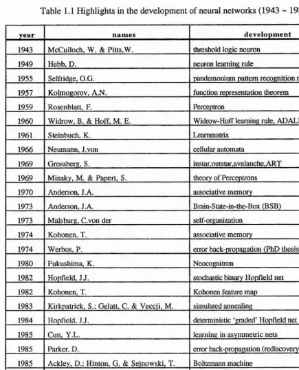
more details about the historical development see those listed in Table 1.1 below in addition to the book (Rumelhart, et ai, 1986).
Table 1.1 Highlights in the development of neural networks (1943 ~ 1987)
year nam es d evelopm ent
1943 McCulloch, W. & Pitts,W. threshold logic neuron
1949 Hebb, D. neuron learning rule
1955 Selfridge, O.G. pandemonium pattern recognition model 1957 Kolmogorov, A,N. function representation theorem
1959 Rosenblatt, F. Perceptron
1960 Widrow, B. & Hoff, M. E. Widrow-Hoff learning rule, AD ALINE
1961 Steinbuch, K. Learnmalrix
1966 Neumann, J.von cellular automata
1969 Grossberg, S. instar.outstar,avalanche,ART 1969 Minsky, M. & Papert, S. theory of Perceptrons
1970 Anderson, J.A. associative memory
1973 Anderson, J.A. Brain-State-in-the-Box (BSB) 1973 Malsburg, C.von der self-organization
1974 Kohonen, T. associative memory
1974 Werbos, P. error back-propagation (PhD thesis)
1980 Fukushima, K. Neocognitron
1982 Hopfield, JJ. stochastic binary Hopfield net
1982 Kohonen, T. Kohonen feature map
1983 Kirkpatrick, S.: Gelatt, C. & Veccji, M. shnulated annealing
1984 Hopfield, J.J. deterministic ‘graded’ Hopfield net
1985 Cun, Y.L. leaining in asymmetric nets
1985 Parker. D. error back-propagation (rediscovery) 1985 Ackley, D.; Hinton, G. & Sejnowski, T. Boltzmann machine
1986 Rumelhart, D.; Hinton, G. & Williams, E. multilayer Perceptron
1986 Szu, H. Cauchy machine
1987 Caipenter, G. & Grossberg, S. Adaptive Resonance Theory (ART) II 1987 Hecht-Nielsen, R. generality of tliree-layer network
[image:20.618.62.497.138.676.2]f
1.3 Sequential processing in neural networks
There are a number of areas in which neural networks can provide adequate models. One area I would like to enhance the capability of neural networks in is modelling sequential behaviour such as time dependent signal processing.
A common task for the Perceptron was to carry out visual character recognition. The sequence underlying the presenting of characters is not intended affect the recognition of those characters. Consequently, this kind of task does not strongly suggest that time should be incorporated into the neural framework. However, it is also clear that the processes of the human brain are not only highly parallel but also sequential. Hearing, for example, is a different task showing a basic human capacity where time sequences are more clearly involved. It is unlike the earlier visual recognition task, since hearing input sequences involves dependence between current and past inputs, and so temporal structure is involved in the hearing processing. This example suggests that time may need to be imposed in neural networks in such a way that assists and enhances the capabilities of sequential processing. Processing involving temporal structure will be called sequential processing henceforth throughout this thesis.
Attention has been paid to the problems of learning sequences in neural networks (e.g. Elman, 1988). However many of the associated problems remain unsolved or at least not fully investigated. It will be put forward that this is at least partly because BP-based learning has typically taken a single weight state to be the result of learning regardless of whether the learning is to approximate an I/O function, dynamic system or I/O associations with an underlying temporal stmcture.
The question being raised is what constitutes general justification for the weight state approach and whether it is justified in all cases. One justification arises from the general principle that with enough hidden units a single weight state can provide I/O mappings of any complexity (Cybenko, 1989; Funahashi,K., 1989; Hornik, K., Stinchcombe, M., and White, H., 1989).
7
Neural knowledge represented through a set of weights as parameters embodied within the system exists together with the system structure. Such knowledge as a set of parameters may be fixed for the long term and so not be intended as a function of time. If the knowledge is to be accessed at any time, this brings a random access feature to the system. Theoretically then, the single weight state approach has the capability to represent any complex long term knowledge and provide a system with random access and a genemlization capability.
However, consider Simpson’s definition of neural convergence (Simpson, 1989):" if the mapping converges to a fixed value, or to some fixed set, then the learning procedure is properly capturing the mapping. “
It would seem from the above that the single goal weight state approach in neural learning is only one of several approaches which might be able to solve tasks. In particular, there may be good reasons not to stick with the single goal weight state approach for solving vaiious kinds of sequential processing tasks.
For example, when only sequential access is required after learning, neural performance may be viewed as drawing upon different knowledge sequentially. Each piece of knowledge can then be adapted to act as a set of parameters for a certain moment in sequence. In this way, an account of the temporal and sequential aspects of processing is used. In this case, there is no reason to restrict the system to find a single instantaneous knowledge state as tlie goal of learning.
1.4 Basic concepts
Fundamental concepts of neural networks used in the thesis are briefly reviewed here. For more details see the papers and books (e.g., Lippmann, 1987; Rumelhart et al, 1986; Crick, 1989; Kinoshita et al, 1987; Tazelaar, 1989).
• An artificial neuron
In a neural network, each unit generally has an output activity that is determined by the input received from other units in the network.
There are many possible variations within this general framework. One common, simplified assumption is that the combined effects of the rest of the network on a unit are mediated by a single scalar quantity. This quantity, which is called the excitation of a unit is usually taken to be a lineai' function of the output activity of the units that provide input to the unit:
X y w (1.1)
j V I (
where xj is the total input to unit j\ yj is the output activity of unit i; wji is the weight value on the connection from unit i to unity ; 9y is the threshold of unit /. The threshold term can be substituted by giving every unit an extra input connection from a common unit called bias whose activity level is fixed at 1. For unity, the weight on this special connection is tlie negative of the threshold 0^. An artificial neuron is shown in Fig. 1.1.
The output activity y/ of unit i can be defined to be a lineai* or nonlinear function of its total input excitation xj. For units with discrete states and a threshold 0, this function typically has value 1 if the total input is great than 0 or 0 otherwise. For units with real-valued states, a typical linear input-output function is: yt = xi, a typical nonlinear input-output function is the logistic function: y = f(x) = 1/ (1+e'^) (Fig. 1.2). Because the latter function is monotonie and “S-shaped”, it is often referred as a sigmoid function.
a
0.5.
X Fig. 1.1 An artificial neuron
• Perceptron procedure
Fig. 1.2 The logistic transfer function
This is a simple learning algoritlim for the Perceptron (Rosenblatt, 1962). If the output of a perceptron unit i is yi, we have:
yj(t) = fh i'LiWjiyi(t) ]
where//î is a step function//,, {x) is 1 if .x > is 0 otherwise. We adapt weights wji at time t+l according the following rules {dj denotes tlie target value of unit j)\
if iyj - dj)
if iyj - 0 bui dj =7) if (yj - 1 but dj =0)
• Delta rule
then wji(t+l) = Wji(t); then Wji(t+1) = Wji(t) + yi(t)\ then Wji(t+1) = Wji(t) - yi(t);
This rule, proposed by Widrow and Hoff in 1960, uses the difference between the desired, or target, activity and the obtained activity, which is called the delta, to drive learning in a network. The idea is to adjust the strengths of the weight connections so that they will tend to reduce this difference or error measure. The rule in its simple form can be written as:
Awji = £- 5j Oi (1.2a)
where e is a constant of proportionality called the learning rate, Oj is the output of unit i which is input to the link Ijj. 5j is the delta for a linear unit./ given by :
0j = tj~Oj (1.2b)
which is the difference between the teaching activity tj (to output unit j) and its actual activity value Oj. There is also though the feature of many patterns being learnt by the
network so that the rule becomes; |
Awji = eZp ôjpOip (l-2c)
11
where Ôjp and oip are defined for each pattern p , where the index p ranges over the set of
the input patterns, and / refers to the source unit for the link Ip. |
The delta rule is very similar to the Perceptron procedure for networks with*threshold units, | the differences are only that units with real-valued outputs instead of linear threshold units
are used in training.
In the perceptron, the error signal is used in the calculation of the modification of weights and is equal to the binaiy difference between the weighted input sum after thresholding and
the desired result. There is no distinction made between the performance and the learning # nile as far as thresholding is concerned.
In the delta rule, there is a distinction. During training, the error signal is equal to the difference between the weighted input sum before thresholding and the desired output. During performance, the same linear thresholded units are used as in the perceptron, with an output of +1 if the weighted sum of its inputs is larger than the threshold or -1 otherwise. In other words, the delta rule modifies connection weights when the weighted sum of the inputs of the neuron is not exactly equal to the binary target, even if the thresholded response is conect.
• Gradient descent
i proportional to the negative of the derivative of the function/ with respect to the variables |
V,-:
In neural networks, gradient descent is used to find a minimum value for the error function E, which depends on some independent variables. In techniques such as BP, we want to find the values of weight variables W where E takes on a minimum value.
• Least-Mean-Square procedure
LMS is an eiTor measure which has been applied by Widrow and Hoff (1960) to give a version of the delta rule. The procedure makes use of the ideas of the delta rule, LMS error and gradient descent for learning and adjusting connection strengths.
12
i
The total eiTor of such a one layer linear network can be defined by a simple error function as in Eq.l.2b or by a quadratic LMS error function such as :
E = S/7 Ep = S/?S( {tpi - Opi )^ (1.3 a)
where tpi denotes the target value of output unit i for pattern p. Gradient descent can be then used to find a weight state that minimises the function E. The procedure is that after each pattern has been presented, the error-weight derivatives for that pattern are computed. The total error-weight derivatives of the patterns are used for making each weight moving down the eiTor gradient toward its minimum value for all the patterns. The learning rule is:
^ d o i d w ' i j
when ÛI = S; OJ wij (for a one layer linear network).
• Network topology
The functional ability of a neural network is largely dependent on its net topology, i.e. the
units, which receive inputs from the network’s environment; the output units, which have associated teaching or target patterns; and the hidden units, which neither receive environment inputs directly nor give direct output to the environment.
Depending on the linking relationship among the units, there are two major different types of networks: feedforward networks and recurrent networks. Networks may not necessarily have all the above tliree kinds of units.
• Feedforward networks and recurrent networks
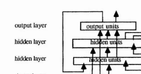
A feedfoi*ward network is a network with all links being feedforward. This implies that all units are linked from units in a lower layer to units in a higher layer (closer to the output layer), no links between units within the same layer. The structure of a fully connected general feedforward network is shown in Fig. 1.3a. Where each unit of each layer is linked feedforward to the units in all the higher layers. Feedforward networks may not necessarily have all those links.
When a feedforward network’s unit of one layer is only linked to the units in the next layer and not to any units in the other higher layers, the feedforward network is a stiictly layered network. As an example, the structure of a strictly layered network is shown in Fig. 1.3b.
There are no above linking limitations in recurrent networks. In recunent networks, there is at least one unit whose output can directly or indirectly feed back into the unit. The structure of a recurrent network is shown in Fig. 1.3c for an example.
hidden layer
input layer | input uniij 1 output units
f
hidden ui iti hidde n UI its
[f
iiidden layer
hidden layer
output layer outpiâ units I hidden units
£ hidden units
I input layer | input units
Fig. 1.3a A general feedforward network Fig. 1.3b A strictly layered feedforward net
— 13
output layer hidden layer hidden layer input layer
i
I output units
hidden units
1
z
Rideen unitsI U lilld A
e
input ^ i t s
Fig. 1.3c A recunent network structure
• Backpropagation learning procedure
The “backpropagation” (BP) learning procedure is a generalization of the LMS procedure that works for non-linear networks which have layers of hidden units between the input and output units. The basic idea of the learning method is to combine a nonlinear perceptron-like system capable of making decisions with the objective error function of LMS and using gradient descent method to minimise the error by finding a set of suitable weight variables.
Variants of the BP procedure were discovered independently by Werbos (1974), Le Cun (1985), Parker (1985) and Rumelhart, Hinton & Williams (1986). They are going to be refeiTed as conventional BP throughout this thesis, all approaches using the BP idea based on a single goal weight state approach will be termed as state-based backpropagation (SBP).
• Batch and on-line
The “batch” version of BP sweeps through all the cases of I/O training tuples accumulating the measure of the derivative of the error function with respect to any weights in the network 3E/9Wij before changing the weights. This is guaranteed to move in the direction of steepest descent at the cuiTcnt weight state.
The “on-line” version, which requires less memory, updates the weights after each input- output case. This version can be made as an arbitrary close approximation of the steepest
[image:28.619.171.408.81.205.2]gradient descent after a complete sweep through all the cases provided each of the weight changes is sufficiently small.
• Local and global (non-local)
These two terms are used to point out what kind of information are needed when a computation is carried out.
Local in computation implies that each unit requires information only from other units to which it connects. When these information are called local information, global in computation implies that some non-local information are needed.
• Error- weight space and error surface
The LMS learning procedure has a simple geometric interpretation. An n+7 multiple dimensional “error-weight space” can be constructed in this way where n is the total number of the weight links in a network ; there is an axis for each weight, and one extra axis coiTesponding to the error measure.
For each combination of weights, there is one weight state in weight space. The network will have a certain eiTor for current inputs which can be represented by the height of a point above a weight state in weight space. These points form a surface called the error-weight surface.
• I/O tuple. I/O path and training position
An 1/0 tuple is a list of input and output values. Each of the values is associated with an output activity of an input or output unit in the network.
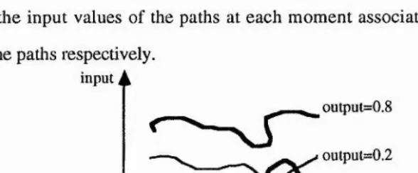
An I/O path, as used throughout the thesis, is comprised of an infinite sequence of 1/0 states. Each of the states is an 1/0 tuple at a certain time. At an instant in time, an I/O tuple in the path is seen whose values aie the cunent associated signal values at that instant.
Each of the individual I/O tuples occurring at the same evolved fractional distance in time along each of a number of I/O paths are at the same training position. The fractional distance is said to constitute a training position in the I/O paths’ state sequences. There are infinite number of the I/O states along each path but only finite number of them are tested or used, which consist of the sequence of the I/O states.
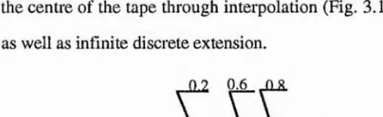
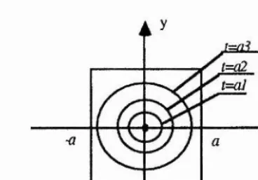
A diagram in Fig. 1,4 shows the relationship between training positions and I/O paths. Suppose the training positions are at ?/, t2 and tk along the time axis. The input axis shows the input values of the paths at each moment associated with three fixed outputs along the patlis respectively.
input À
output=0.i
output=0.2 output=0.6
time
Fig. 1.4 A diagram of showing the relationship between paths and time
• Fixed-point and non-fixed-point algorithms of recurrent networks
Fixed-poini algorithms enable kinds of dynamic behaviour which are designed to have the networks converge to some stable fixed-points in error-weight space. In particular, when an input pattern is given either as an initial condition (when a network has no input units) or as a constant external input, the response of the network is taken to be the output state of the network once it has reached its fixed-point.
Non-fixed-point algorithms on the other hand are able to learn non-fixed-point attractors in time and to produce desired sequential behaviour over a bounded interval.
[image:30.617.117.411.284.406.2]• Time dependent signai processing
In this thesis, time dependent signal processing is defined as processing which involves arbitrary approximation of I/O associations chosen along a number of I/O paths.
• Weight state path and goal weight state path
The weight state path, as used in the thesis, is an infinite sequence of weight states consisting of finite goal weight states and infinite interpolated weight states. Each of the state is a set of weight values; each value is associated with each link in the network.
Each goal weight state belonging to the weight path is associated with each trained I/O training position. Such a state enables the network to act as a machine which produces the correct outputs for any inputs associated with the position. Each interpolated weight state belonging to the weight path is associated with each untrained position, it also enables the network to act as a machine which approximates the correct outputs for any inputs associated with the position.
The goal weight state path is an ideal weight state path, each state along the path is the goal weight state of the associated training position.
• Temporal association
Temporal association is that a particular output sequence is produced in response to a specific input sequence.
1.5 Outline of the thesis
This thesis includes the review, analysis, design, implementation and empirical assessment of learning models for solving problems involving sequential I/O associations where analogue values may be involved. The models involve multiple layer networks based on backpropagation as the core part of the learning method. The efforts made in the
approaches are purely conceptual and methodological using artificial neural networks, no other biological or psychological plausibilities are consideæd.
In Chapter 2, a general review is given to assess the capability of the existing neural models in learning sequences. A detailed discussion on ten related models is presented. This gives an insight of what is the inherent sequential processing capacity of those models.
In Chapter 3, It is argued that a new framework is needed. This is through both reviewing related features of signal processing and analysing the inherent infeasibilities in training and generalization for arbitrary approximation I/O signal associations underlying continuous analogue functions using SBP approach. The philosophy of a new path-based framework investigated in the thesis is presented.
In Chapter 4, a new approach using the new path-based framework called feedforward continuous back-propagation (FCBP) is presented. The aim of the FCBP approach is to provide a means for achieving arbitrary approximation of analogue signal associations within a fixed neural topology. The notion of goal weight sequences is introduced and applied; the training and generalisation capabilities of FCBP are analysed; the training and generalization schemes of FCBP are given.
In Chapter 5, another path-based approach called recurrent continuous backpropagation (RCBP) is presented. RCBP is a kind of path-based dynamic system. The notion of activity sequences is introduced; the design and implementation details of the model are described; the training and generalization schemes of RCBP are given.
In Chapter 6, several experiments based on FCBP and RCBP are presented and the results aie analysed. These experimentations are chosen not only to show the features of the two models but also to demonstrate the capabilities and benefits for training and generalization by employing the concepts and methodologies embodied in the two new models.
In Chapter 7, a simulator called cbptool is introduced here. This chapter is a guide of how the design of cbptool has been evolved from conception and requirements for
implementation. A detailed description of the functions, designing, internal representations and user interfaces of the tool is given. Possible improvements in the design of the tool are also discussed.
Finally in Chapter 8 a general conclusion is made based on the thesis. This includes reviewing the general points of the research and recommending some future work.
2.2 TIME REPRESENTATION IN NEURAL NETWORKS
Neural networks are parallel distributed processing systems. Because of the parallelism, learning sequences implies a time representation problem (Elman, 1988).
In the conventional serial processing computer system, the question of how to represent time interacting with sequential tasks generally does not arise. There is no such question
— 20
CHAPTER 2
SEQUENTIAL PROCESSING USING STATE-BASED BP MODELS
2.1 Introduction
As it is discussed in §1.3, this thesis is about investigation of the capability of neural networks in dealing with sequential processing. Many approaches have been investigated to strengthen this capability in neural networks. Three main kinds of approaches have been used to explore the problem of learning sequences using neural gradient descent methods. The first one is a simple spatial approach. This is to represent time as an explicit part of inputs (§2.2.1). The second kind is to impose dynamic features in networks through special network topology (§2.2.2). The third kind of approach is to employ complex
dynamics to train networks to be dynamic systems which can continuously react to the | sequences of inputs for temporal associations (§2.2.3).
because sequential tasks are processed step by step in succession where sequences of processing represent sequenced events. Compared with the traditional serial computer system, neural networks have a major difference in dealing with sequences. For traditional computer systems, a finite internal state representation is automatically present. In neural network models, a time representation problem needs to be solved explicitly for learning tasks which involve internal state sequences. In general there are three types of tasks related to the problem of learning time sequences in neural networks, which are sequence recognition^ sequence reproduction^ and temporal association. Temporal association is a general case, it includes pure sequence generation and the previous two cases as special cases.
Many methods for implementing the above three tasks in neural networks have been investigated. In this thesis only the approaches based on the SBP framework will be concerned. It can be seen that the way of representing time in those SBP based models is various. This section will discuss the three major methods mentioned in §2.1: representing time spatially; imposing internal states using special network topology; embodying more complicated dynamic features in fully recunent networks.
2.2.1 THE SPATIAL REPRESENTATION OF TIME
This method is to treat the effect of time as an explicit part of the inputs, in other words to represent the effect of time as additional inputs. Typically this approach uses a pool of input units for the event presented at time t, another pool for t+1, and so on in what is
^Sequence recognition is that a network produces a particular single output value when a specific input sequence is presented.
^ Sequence reproduction is that a network is able to generate tlie rest of a sequence itself when it sees part of the sequence.
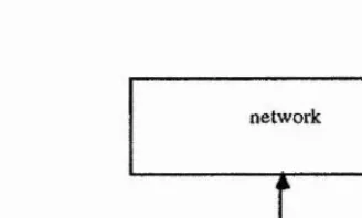
often called a ‘moving window’ paradigm. Time is represented explicitly by associating the serial order of the pattern with the dimension of the pattern vector. The first temporal event is represented by the first element in the pattern vector, the second temporal event is represented by the second element in the pattern vector and so on. Each entire window is thus processed as a single parallel input tuple by the model (Fig. 2.0). A model called time-delay neural network (TDNN) has been investigated based on this idea which will be reviewed in §2.3.1.
network
pattern vector
[image:36.616.198.362.235.334.2]I St pool n th pool
Fig. 2.0 The diagram of spatial representation model
This spatial representation method may be used for solving some sequence recognition problems as it can produce a particular output pattern for a number of input sequences with a fixed length. This method has been applied to speech recognition (e.g., McClelland and Elman, 1986; Cottrell, Munro & Zipser, 1987; Waibel et al., 1989 ). However, the system needs to memorise an entire fixed length sequence which has proven itself to be unsatisfactory in solving sequence recognition problems in general. This is because many tasks do not know the length of all related sequences, or do not have all sequences with a fixed length. As Elman (1988) pointed out, such implementation is not psychologically satisfying, and it is also computationally wasteful since some unused pools of units must be kept available for the rare occasions when the longest sequences are presented. Therefore, the models based on this time representation can only be applied to a limited number of real tasks. This representation is thus not a necessarily natural or practical method for analogue temporal stmcture tasks in neural networks.
2 .2 .2 DYNAMIC SYSTEM APPROACHES - SPECIFIC TOPOLOGIES
There are other two major methods used for learning time sequences. Both are trying to give processing systems some designed dynamic properties to represent temporal states or to represent time by the effect which time has on processing. This is to have the effect of time implicitly in a network by introducing some internal states for the network.
One of the methods is to approximate dynamic systems through specific network topologies that have internal states to represent time sequences. The other is to approximate dynamic systems by providing the processing system with more complicated dynamic i*ules than the topology approach.
[image:37.616.197.365.581.670.2]As an example, the following shows how internal states can be imposed and used effectively in a specially designed network. Suppose a two input unit network is required to do sequential binary addition for two binary input sequences. The structure of the network has been designed and shown in Fig. 2.1, with a suitable learning algorithm described in §2.3.2.1. In this network, two inputs are used for representing the current input values from the two binary sequences, the previous inputs and their effects in time can be aggregated in a carry unit Uc by its state so that the inputs from the immediate past are available as well as cuiTent inputs; that is, delayed inputs are available. The system thus decides the output at time t according to the two explicit inputs at t and the implicit input from the internal state, which is the state of the cany unit.
Fig. 2.1 The network for two string binary addition
" i
From the understanding of what the model can be used to learn to be instead of how to learn, some discussions can be made based on this kind of neural model.
^ Here we define dial an one-many association in neural networks is that for a single input tuple, die networks have different output tuples associated with it.
_ 24 —
1
From the topology structure used in the above example, it is noticed that networks with a limited set of carefully chosen recurrent connections are very interesting. When output
from a network system is fed back into the network as an extra input, this may enable the .# network to learn and to choose the next output in a way at least partly based on the previous
one. These recurrent links (here the link from U5 to Uc ) can help to provide internal states for the networks and hence a dynamic system even when the simple learning rules applied in the associated feedforward networks are used. Some models which have been investigated for this purpose will be discussed in §2.3.2.
2 .2 .3 DYNAMIC SYSTEM APPROACHES - SPECIFIC DYNAMIC RULES
As mentioned in the last section, another method for dealing with temporal structure problems is to further study the dynamic features embodied in fully recurrent networks. This is one of the steps towards representing more complicated temporal structures in neural networks.
The following is a review of why a recurrent network is needed for this dynamic system approach. If a network is able to do one-many^ associations, it implies there are some internal states in the network. If we view the activity value of each neuron in a network as
the only source of the internal states of the network, when the network can do one-many -associations, this implies that some neurons' activity states have many different values
activity value for the same weight state when the inputs of the network are the same, so that there is no such kind of internal state in any feedforward networks, no feedforward networks can have one-many associations in SBP.
However in SBP networks can have some internal states when there are some extra inputs beside the inputs from input neurons to networks. Some dynamic features may be imposed into networks with recurrent links to have this capability. The major features of recurrent networks can be concluded as follows:
A logistic gradient-descent approach in Cartesian coordinates for recurrent networks is an approach based on non-linear system with dynamic features. Exploration of recurrent networks is to study dynamic systems of neural network sort. Recurrent links in a network may allow the network to have internal states and produce complicated, time-varying outputs in response to a simple input. So recurrent networks may be used to approximate not only a foimal automaton but also more complicated potential phenomena.
Note that recurrent networks intuitively can be used for embodying internal states and representing time dynamically through imposing on a suitable dynamic rule. However the network topology is not the sufficient condition of having a dynamic system. Pineda (1987), Almeida (1987), Rohwer and Forrest (1987) have independently derived an equivalent algorithm called recurrent back-propagation for fixed-point recurrent networks. This is a learning algorithm based on recurrent networks, and a step to show that conventional back-propagation can be extended to arbitrary networks. Because this algorithm is only for recunent networks which can converge to stable states, this model cannot be used for problems related to learning time sequences. It can be seen that the dynamics imposed on a network will decide the capabilities of the network.
Two existing approaches mentioned in §2.2.2. and §2.2,3 can be concluded as this: the first one is a simple rule based dynamic system approach which is based on some specific designed network topologies; the second one is to impose various dynamic rules and study complex dynamic features by making full use of the inherent dynamic properties in a fully
— 26 —
recurrent network. In other words, the first is a topology based approach which embodies internal states through specially an anged recurrent links and context units. The second one is a rule based approach which is to control the approximation of target trajectories by imposing different ways of error propagation through time.
One common feature of the above three approaches is that they are all trying to represent time sequences instead of to model the sequences in the parallel processing systems. Models based on the three approaches for learning time sequences have been proposed and investigated. Next section is ananged to review those typical models.
2.3 MAJOR APPROACHES
Particular methods according to the types described in §2.2 are reviewed here.
There are two major common features in all these existing approaches reviewed here: (1) After training finished, all the networks converge to a single weight state; (2) gradient- descent is used as an error correction method. Differences between these approaches include: different dynamic rules are used by those models; some of the approaches are on line and some are on batch; some of the approaches are based on discrete time and some based on continuous time; some are local and some are global. The major features of each of these approaches will be reviewed next.
2.3.1 TIME-DELAY NETWORKS
As reviewed in §2.2.1, the simplest way to perform sequence recognition is within the paradigm of spatial representation: this is by turning the temporal sequence into a spatial pattern on the input layer of a network. A feedforward network and the backpropagation learning algorithm can then be used to learn and recognize sequences.
can have two dimensional time representation, one from the spatial representation of input patterns and another from the whole pattern shifting k times.
For example, the values x(ti), x(ti-A), x(ti-2A), ... x(ti-(k-l)A) from a signal x(t) will be presented simultaneously at the input of a network with k time delay as one pattern for training. In a practical network, these values could be obtained by feeding the signals into a temporal window with a fixed size k and position for each time slice as shown in Fig. 2.0.
A TDNN can be implemented in a replicated feedforward network trained under constraints. The replication implies that each input unit has multiple copies (each associated with a particular time step) and uses a sepaiate weight from each of the copy to each hidden unit, each link canies information about activation at a particular time step, to impose a kind of temporal window on the system — i.e. on the size of the number of time delay links. The network can be trained under constraints which ensured that the multiple copies of each unit applies the same set of weight to each part of the temporal window.
During training, all weights associated with different time frame but the same time delay will have the same set of values, this constrained training in a replicated feedforward network can be achieved through using a regime very similar to the conventional backpropagation (e.g. Lang & Hinton, §4.3, 1988; Lang, 1989) or the regime applied in the backpropagation through time (§2.3.3). Since a hidden unit applies the same set of weights at different time frames after training, it can then produce similar responses to similar patterns that are shifted in time.
For example, a set of sequences is with 12 time steps, suppose the number of the time delay is 3 (or the size of the temporal window), then 10 training patterns need to be trained for each of the sequences in TDNN using a multiple layer replicated feedforward network shown in Fig.2.2 using constrained training algorithm, three sets of weights between input and hidden units can then be applied in perfoimance.
Although the power of this model was demonstrated by showing a better performance than all previously tried techniques on some speech applications (Waibel, 1987), several drawbacks to this general approach to sequence recognition were also reported (Mozer,
1989X
Fig. 2.2 The constrained weights feedforward net
The length of the delay must be chosen in advance to accommodate the longest effective sequence because the length detennines how many context information can be provided for recognition. This model cannot be used for sequence recognitions with arbitrary length of context. And perhaps most important in signal processing, the input signal must be properly registered in time and aiTives at the exactly coiTect rate. This model may thus only be used for solving some particular sequential recognition problems.
2 .3 .2 PARTIALLY RECURRENT NETWORKS
Another way to recognize and reproduce sequences is using partially recuiTent networks. These networks use special topologies as described in §2.2. Three models are reviewed here.
2.3.2.1 Jordan networks
Jordan (1986) described a network containing the feature of internal states in a specially designed partially recunent network.
The general structure of this kind of network is shown in Fig. 2.3a; a network showing more unitary details of the structure in Fig.2.3b ( not all links are shown). It can be seen that the basic structure of the Jordan networks is similar to a feedforward layered neural
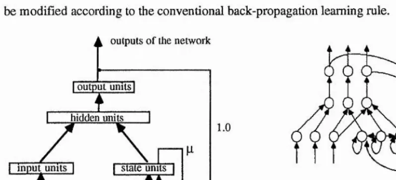
network. The additional part is to augment the basic feedforward layered structure at the input level with some additional units called state units which provide limited recurrence. The number of the state units is equal to the number of the output units so as to buffer the output state of the output units. This is achieved when each state unit receives a connection with a fixed weight of 1.0 from its corresponding output unit. At the same time, the state units also send connections with learnable weights to all hidden units and with a chosen weight of |i to all state units (including self-connection) to provide states. Except those specially an anged links, all the other links of the network are learnable and the weights can be modified according to the conventional back-propagation learning nile.
outputs of the network
I o u t m t u n its I
hidden units
I inpu^units I
inputs of the network
state units
!
1.0
Fig. 2.3a A Jordan Recunent Network Fig. 2.3b The structure of the Network
In the network, the output states of the state units are derived from their own outputs and those of the output units on the previous time cycle. This allows the current state to depend on the previous state and on the previous output. The state at time t is given by:
St = ]lI St-] + y t , i ( Z l )
where St and denotes respectively the state vector and the network output vector at time t; ji (|i<l) is the strength of the self connections. Iterating Eq. (2.1), we have:
St
=
yt-i+
m - 2 + yt-3 y2+
Vo = I
i^^'ht-rr = l (2.2)
It can be seen lliat the self connections give state units themselves some individual memory. According to Eq. (2.2), fi value helps to define the state as an exponentially weighted average of past outputs, so that the arbitrarily distant past has some representation in the state. The value of p. decides the decay rate of past information. By making p closer to 1 the memo l'y can be made to extend further back into the past. In general the value of p should be chosen to suit the features embodied in the input sequences (Stornetta et al.,
1987).
In this way state units memorise outputs of the network at the previous time cycle; they act as internal states imposed in the network. The known internal states which can be leaint during training then can be used in the network. The current network outputs are dependent on not only the current inputs but also the internal state — the previous state. This enables the subsequent behaviour to be shaped by previous responses.
This kind of network can be used to solve certain tasks which involve learning and representation of infonnation contained in sequences. Some successes have been reported when the network is trained to generate a set of output sequences with a fixed input pattern; to prompt different output sequences with different input patterns (Jordan, 1986); to distinguish different input sequences (Anderson et al., 1989).
In this model, the internal states to be retained by the network across time must be manifested in the desired outputs of the network after a certain time. This is because the internal states are produced tlirough the actual outputs of the network (see Eq.(2.1)). This means that only a certain type of temporal sti uctures can be represented in the networks.
2.3.2.2 Elman simple recurrent network
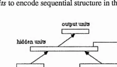
Another kind of partially recunent network architecture has been studied based on Jordan's approach. In 1988, J. Elman investigated what he called a simple recurrent network (SRN). A general structure is shown in Fig.2.3c.
The basic structure of SRN is also similar to a feedforward layered neural network. At the input level there are also some additional units which provide limited recurrence similar to that in Jordan networks, but they are called context units. The number of the context units is equal to the number of the hidden units so as to act as a buffer with the copy of the output state of the hidden units. Each context unit receives a connection with a fixed weight of 1.0 from its corresponding hidden unit and sends connections with learnable weights to all hidden units. This network copies the output values of the hidden units into the set of context units to encode sequential structure in the network.
output uiüts
hidden units ,---J O
[ :.::zzn
c
[image:45.616.181.377.285.397.2]input units context units Fig. 2.3c Simple Recurrent Network
In Jordan’s network the state of the context units consists of the outputs of output units of the previous time cycle and self-connections. In SRN hidden units are used to represent a compressed form interior structure. This is that the state of the context units was derived from the outputs of hidden units on the previous time cycle. In contrast to the output units, as the hidden units are not taught to assume specific values, this means that they can develop representation, in the course of learning a task, which encodes the temporal stmcture of the task.
When using this kind of neural network architecture, the output values of the context units il at time t+1 are the same as the output values of the hidden units at time t. Thus the context
units are able to remember the previous internal state. The context units provide the network with memory by developing internal representations which are sensitive to temporal context. The hidden units have the task of mapping both an external input and the previous internal state to some desired output.
The SRN model has been applied to some tasks which involve sequence recognition. It has been shown in D. Schreiber’s paper (Servan-Schreiber et al, 1988) that a SRN could learn to be a finite state recogniser for a grammar. This is because the encoding of sequential structure depends on the fact that back-propagation enables hidden layers to encode task-relevant information (using hidden units to compress temporally interior structure). In the network, internal representations encode not only the prior event of the network state, but also the relevant aspect of the representation that was constructed in predicting the prior event from its predecessor. When fed back as inputs, these representations provide information that allow the network to maintain prediction-relevant features of an entire sequence. The hidden unit patterns can possibly achieve an encoding of the entire sequence of events presented with finite length. Therefore with enough hidden units, like some other approaches, this model can be applied to train a network to be a finite state automaton.
However, it is noted that die number of time steps of history being maintained relies on the number of the hidden units. So the question with SRN is whether the error from the histoiy that has been cut off is significant. This question can only be answered respect to a particular task. This implies that in SRN the computational expense per time step scales linearly with the number of time steps of history being maintained, because the greater the number of steps maintained, the more hidden units are needed. This can cause problems for both the training feasibility or the amount of storage in SRN. So that it is very likely that the accuracy of approximation is gradually traded off against storage and computation in this kind of network.
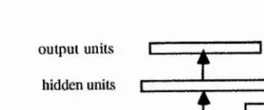
2.3,2.3 Stornetta network
units are the external inputs and themselves, hence network external inputs only reach the rest of the network via the context units. This implies that the inputs to the network are preprocessed by the context units. This preprocessing serves to include past features of the inputs into the present context values, hence letting the network recognize and distinguish
different sequences.
output units i à I hidden units i ^ I
[image:47.612.180.370.189.268.2]context units i
Fig. 2.3d A structure of Stornetta’s network
Some other architectures along the line of the specific network topology approach have also been investigated. Because the scope of this thesis, more discussions about those models can be referred to the review paper given by Shimohara etal. (1988).
It is concluded that: through employing a set of specifically airanged recurrent connections, the partial recurrent networks can show some important features for imposing time structure into neural networks without changing the conventional feedforward learning mle. Similar behaviour can probably be obtained through any of the three partial recurrent networks discussed above. This is regardless of whether the feedback is from a hidden, a output or a context layer, though particular problems might be better suited to one rather than the other.
2.3.3 DISCRETE BACKPROPAGATION THROUGH TIME
The networks reviewed above for sequential processing are either feedforward or partially recurrent networks. Now let us see the models based on fully recurrent networks, in which each unit may be connected to any units.