Stochastic resin transfer molding process
M. Park∗ and M.V. Tretyakov†
Abstract. We consider one-dimensional and two-dimensional models of the stochastic resin transfer molding process, which are formulated as random moving boundary problems. We study their properties, analytically in the one-dimensional case and numerically in the two-dimensional case. We show how variability of time to fill depends on correlation lengths and smoothness of a random permeability field.
1. Introduction. Over the last few decades the use of fiber-reinforced composite materials in aerospace, automotive and marine industries, in sports and other areas has seen a signifi-cant growth. The main benefits of composites include their lightweight and high-performance
nature, as well as their flexibility to accommodate complex designs (see e.g. [4, 2, 10] and
references therein). One of the main manufacturing processes for producing advanced com-posites is resin transfer molding (RTM), which belongs to the Liquid Composite Molding class
of composite manufacturing processes. RTM has five main stages [4,2,23,7]: (i)
manufactur-ing of a reinforcmanufactur-ing preform (e.g., from carbon fiber, glass fiber or other fabric); (ii) packmanufactur-ing the preform in a closed mold, which has a cavity with the shape of the designed part; (iii) injecting resin into the mold cavity to fill empty spaces between fibers; (iv) resin curing (it can start during or after the injection stage); and (v) demolding, i.e., taking the solidified part, after completion of curing, from the mold. In this work we will consider the third stage (filling the preform by resin) only and we will, for simplicity, assume that resin curing starts after completion of the filling, or in other words, that the filling process is much faster than the curing, which is a common assumption for RTM. The injecting resin stage is crucial for getting the expected properties of a material.
It is widely accepted (see e.g. [13,14,18, 24, 26, 29, 40, 49, 54] and references therein)
that composite manufacturing processes are accompanied by uncertainties. The origins of these uncertainties include (a) variability of fiber placements due to imperfections of stages (i)-(ii) of RTM; (b) variability of fiber properties; (c) variability of resin properties; and (d) variability of environment during stages (i)-(iv) of RTM. Deviations from the design caused
by uncertainties can result in defects, which have two manufacturing consequences [2, 24].
First, to avoid compromising performance of the material due to possible defects, one usually uses more conservative designs, making composites thicker and hence more expensive and less lightweight. Second, defects (e.g. dry spots) can lead to a relatively large amount of scrap which increases the cost of the material. Being able to quantify these uncertainties is highly important for further advances of composite manufacturing.
The above-mentioned variabilities usually cause uncertainty of permeability/hydraulic conductivity, which in its turn leads to variability in mold filling patterns and filling times in RTM. In this paper our main focus is on dependence of variability of filling times on properties
∗
School of Mathematical Sciences, University of Nottingham, University Park, Nottingham, NG7 2RD, UK
†
of random fields which model uncertainty of hydraulic conductivity.
Estimation of a filling time for each particular design of a composite part is important for a successful manufacturing process. The filling time should be neither too short nor too long. On the one hand, it should be sufficiently long to allow adequate impregnation of the fibers. On the other hand, a too long filling time can lead to premature gelation (or even solidification) of the resin, which should be avoided as it is a source of defects. Further, a large variability of the filling time is, practically, highly undesirable as it affects robustness of the technological process, making it difficult for automation and standardization (e.g., of an operator’s guidance). Thus, understanding of factors influencing filling time variability is of importance for fiber-reinforced composite manufacturing.
We start (Section2) with considering a stochastic one-dimensional moving-boundary
prob-lem, where analytical analysis is possible. The hydraulic conductivity is modelled as a sta-tionary log-normal random field. In particular, we observe that though the mean filling time does not depend on correlation length of hydraulic conductivity, the filling time variance (as a measure of variability) does depend on the correlation length. We also consider depen-dence of variation of the filling time on smoothness of the random hydraulic conductivity. In
Section 3 we formulate two variants of a two-dimensional moving-boundary problem with a
random hydraulic conductivity tensor. In some previous related works (see e.g. [42, 54]) on
stochastic moving-boundary problems, it was assumed that the random hydraulic conductiv-ity is isotropic. However, permeabilconductiv-ity (and hence hydraulic conductivconductiv-ity) is anisotropic by
design in most cases of practical interest (see e.g.[8,37,30]). Moreover, geometric variability
(i.e., deviations from the design such as variation of gaps between fiber yarns, variation of width and angles of fiber yarns in comparison with design, etc.) was observed in experiments
(see, e.g. [39,18,24,26] and references therein), which gives further evidence for the need to
model hydraulic conductivity as an anisotropic random field. The main difficulty in modeling 2- and 3-dimensional resin transfer processes is the possibility of dry spot appearances, i.e., forming enclosed areas with moving fronts behind the main front. The enclosed areas contain air, which is a compressible medium, while resin can be considered incompressible. A full de-scription of this phenomenon requires a two-phase model involving both incompressible and compressible phases, which is too computationally demanding. Here we work with a reduced model in which the air entrapment is taken into account by modifying the boundary
condi-tions on the internal fronts. A discrete-type version of such a model was proposed in [23] (see
also [2]). Here we formulate its continuous analogue. We note that though our study is
moti-vated by technological processes in production of composite materials, the considered models
are also useful for other porous media problems (see [8, 37,42] and references therein). The
two-dimensional model is solved numerically using the control volume-finite element method
(CV/FEM) which we present for completeness in Section4. The results of our numerical study
of the two-dimensional stochastic moving-boundary problem are given in Section5, where we
also experimentally examine convergence of the CV/FEM algorithm with the quantities of interest being the filling time and void content. A discussion and concluding remarks are in
Section6.
2. One-dimensional model. We start with studying a one-dimensional moving-boundary model for a stochastic RTM process. In what follows we assume that we have a sufficiently
rich probability space (Ω,F, P). Let K(x) = K(x;ω) be a random hydraulic conductivity
defined on [0, x∗]×Ω and taking values on the positive real semi-line. Assuming the resin’s
incompressibility, the moving boundary problem for the pressure of resinp(t, x) takes the form
[2,42]:
− d
dxK(x) d
dxp(t, x) = 0, 0< x < L(t), t >0,
(2.1)
p(0, x) =p0, x∈(0, x∗], p(t,0) =pI, t≥0, d
dtL(t) =−
K(L(t))
κ d
dxp(t, L), L(0) = 0, p(t, L(t)) =p0, t >0,
where L(t) is the moving boundary, κ > 0 is the medium porosity, pI is a pressure on the
inletx= 0,andp0≤pI is the pressure at the outletx=x∗.
We recall that the hydraulic conductivityK can be expressed as
(2.2) K= k
µ,
wherek is the permeability of the medium andµis the viscosity of the resin.
Remark 2.1. For simplicity we assume that the porosity κ in (2.1) is constant. Porosity
can be assumed constant when its variability is significantly smaller than variability of hy-draulic conductivity, which is often the case (see e.g. [8, 37]). It is possible to modify the arguments of this section for the case of random porosity but we do not consider it here. Also, for definiteness, we impose the constant pressure condition at the inlet but other boundary conditions (e.g. constant rate) can be also considered.
Remark 2.2. We note that without losing generality we can putp0 = 0in (2.1) (i.e., either
it is vacuum on the outlet or p is considered as the relative pressure) but for the sake of the two-dimensional model considered in the next section, it is convenient to keep the parameter
p0.
Let
F(y) :=
Z y
0
dz K(z).
Assumption 2.1. We assume that the random field K(x) =K(x, ω), (x, ω)∈[0, x∗]×Ω,is
such that
(i) K(x)>0for x∈[0, x∗]and all ω∈Ω;
(ii)the integral
G(x) :=
Z x
0
F(y)dy
exists for x∈[0, x∗]and a.e. ω∈Ω.
Proposition 2.1. Let Assumption 2.1 holds. Then the unique solution of (2.1) is
L(t) =G−1((pI−p0)t/κ),
(2.3)
p(t, x) =pI−(pI−p0)
F(x)
F(L(t)), t≥0, 0≤x≤L(t), a.s.
Note that Assumption 2.1 implies that G(x), x ≥ 0, is a.s. continuous and strictly
in-creasing, which guarantee existence of the inverseG−1(·), needed for (2.3). We also remark in
passing that if dynamics of the frontL(t) are given then the nonlinear problem (2.1) becomes
linear.
As we mentioned in the Introduction, from the application’s point of view, an important
characteristic is the time τ = τ(ω) to fill a piece of material of length x∗, i.e., the random
timeτ such that
(2.4) L(τ) =x∗.
It follows from (2.3) that
(2.5) τ = κG(x∗)
pI−p0
.
It is natural to assume that the mean ofK(x) corresponds to the hydraulic conductivity
intended by the design of a composite part and the perturbation of this mean is a stationary random field which models uncertainty due to the manufacturing process. Let us now consider
the case of the hydraulic conductivityK(x) being a stationary log-normal random field, which
is a commonly used assumption (see, e.g. [29,18,24,44,54]), i.e.,
(2.6) K(x) =K0exp(ϕ(x)),
whereK0 >0 andϕ(x) =ϕ(x;ω),(x, ω)∈[0, x∗]×Ω, is a stationary Gaussian random field
with zero mean and covariance function r(x).Note that
EK(x) =K0exp
1 2r(0)
,
(2.7)
VarK(x) =K02exp (r(0)) [exp (r(0))−1],
Cov(K(x), K(y)) =K02exp (r(0)) [exp (r(x−y))−1].
The filling time according to the design is equal to
τdesigned= κ
x2
∗
2(pI−p0)EK
.
The first condition in Assumption 2.1 is obviously satisfied byK(x) from (2.6). To satisfy
the second condition, it is sufficient to require that realizations of ϕ(x) are continuous with
probability one and we make the following assumption.
Assumption 2.2. We assume that the stationary Gaussian random field ϕ(x)has zero mean and continuous covariance function r(x) such that for some C >0 and α, δ >0 :
(2.8) r(0)−r(x)≤ C
|ln|x||1+α
for all x with |x|< δ.
Under Assumption 2.2 the random fieldϕ(x) has continuous sample paths with probability
one (see e.g. [1]).
ForK(x) from (2.6), we obtain the following statistical characteristics of the filling time:
Eτ = κ
2(pI−p0)K0
exp
1 2r(0)
x2∗,
(2.9)
Varτ = κ
2exp (r(0))
(pI−p0)2K02 "
Z x∗
0 Z x∗
0 Z y
0 Z y0
0
exp r(z−z0)
dzdz0dydy0− x
4
∗
4
#
.
To understand the behavior of Eτ and Varτ in terms of K(x), it is convenient to re-write
(2.9) via the mean and variance ofK(x):
Eτ = κx
2
∗
2(pI−p0)
EK2(x)
[EK(x)]3 =
x2
∗κ
2(pI−p0)EK(x)
VarK(x) [EK(x)]2 + 1
,
(2.10)
Varτ = κ
2hVarK(x) [EK(x)]2 + 1
i2
(pI−p0)2[EK(x)]4 Z x∗
0 Z x∗
0 Z y
0 Z y0
0
Cov(K(z), K(z0))dzdz0dydy0.
(2.11)
It is interesting that the mean filling time depends only on VarK(x) and EK(x) and does
not depend on the covariance, and hence it does not depend on the correlation length and
smoothness of the random fieldK(x).We pay attention to the interesting fact thatEτ grows
linearly with VarK(x).
The variance of the filling time Varτ depends on covariance ofK(x). Then to understand
its behavior with respect to correlation length and smoothness of K(x),let us consider some
particular cases ofϕ(x).
First let us look at the simple case of ϕ(x) being independent of x, i.e., being just a
Gaussian random variable with zero mean and varianceσ2 which can be viewed as a perfectly
correlated medium. Then
(2.12) Varτ = κ
2x4
∗
(pI−p0)2[EK(x)]4
VarK
[EK]2 + 1
2
VarK,
i.e., Varτ grows cubically with increase of VarK in this case.
Remark 2.3. In this case of a perfectly correlated medium we also have from (2.5):
EK = κx
2
∗
2(pI−p0)
E1 τ,
(2.13)
VarK = κ
2x4
∗
4(pI−p0)2
Var1
We note in passing that (2.13) is often used in experiments for estimating an effective macro-scopic hydraulic conductivity (and hence effective permeability) via observing time to fill of samples of a material (see e.g. [26]). But it is not difficult to see that when the hydraulic conductivity is not perfectly correlated, (2.13) might not be a good way to estimate the mean and variance of hydraulic conductivity (cf. (2.10)-(2.11)).
Now consider the following Mat´ern covariance function for the stationary Gaussian random fieldϕ(x) (see [25,51,41,35]):
(2.14) r(x) =σ2 1
Γ(ν)2ν−1 √
2νd(x, λ)νKν
√
2νd(x, λ),
where Γ(·) is the gamma function, Kν(·) is the modified Bessel function of the second kind,
σ2 is variance,ν >0 is a smoothness parameter, λ > 0 is a characteristic correlation length,
and d(x, λ) is a scaled distance function. In particular, we have
(ν = 1/2) r(x) =σ2exp (−d(x, λ)),
(2.15)
(ν = 3/2) r(x) =σ21 +√3d(x, λ)exp−√3d(x, λ),
(2.16)
(ν = 5/2) r(x) =σ2
1 +√5d(x, λ) +5 3d(x, λ)
2
exp−√5d(x, λ),
(2.17)
(ν → ∞) r(x) =σ2exp −d(x, λ)2
.
(2.18)
The parameterν in the above covariance functions controls the degree of smoothness of
sam-ple paths of the random field. The random fieldϕ(x) with Mat´ern covariance function (2.14)
has dν−1e sample path continuous derivatives with probability one. Hence, with the
expo-nential covariance function r(x) from (2.15), the random field ϕ(x) has continuous (but not
differentiable) sample paths with probability one; withr(x) from (2.16) – once differentiable
sample paths with probability one; withr(x) from (2.17) – twice differentiable sample paths
with probability one; and with r(x) from (2.18) – infinitely many times differentiable sample
paths.
Note that we will use the four Mat´ern covariance functions in this section for x being
one-dimensional and in the next sections for x being two-dimensional. The scaled distance
of the form d(x, λ) = |x|/λ, with |x| being the usual Euclidean distance, corresponds to an
isotropic random field. In the two-dimensional case considered later in the paper we also model the random conductivity as an anisotropic random field, appropriately choosing the scaled distanced(x, λ) (see Section 5).
We recall (cf. (2.9)) that the mean filling time does not depend on the choice of covariance
and hence, in particular, it is the same for all four Mat´ern covariance functions (2.15)-(2.18).
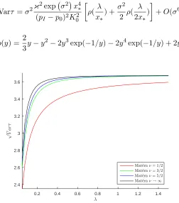
It is not difficult to show that, in the case of these Mat´ern covariance functions, variance Varτ
of the filling time has the following properties: (i) it is increasing with growth of the correlation lengthλ; (ii) for small correlation lengths relative to the size of the materialx∗/λ >>1,Varτ
grows linearly withλ; (iii) for large correlation lengthsx∗/λ <<1,Varτ is almost independent
ofλ(note that in the case of a perfectly correlated medium we had (2.12)); and (iv) for a fixed
λ, variance Varτ of the filling time grows with smoothness of the random field. We illustrate
these properties in Fig.2.1.
As an example, we also give the expansion of Varτ in the case ofν = 1/2 and smallσ >0
(expansions in small σ of statistical moments of the interface dynamics and of the pressure
were derived in [22]):
Varτ =σ2κ
2exp σ2
x4
∗
(pI−p0)2K02
ρ( λ
x∗
) +σ
2
2 ρ(
λ
2x∗
)
+O(σ6),
where
ρ(y) = 2
3y−y
2−2y3exp(−1/y)−2y4exp(−1/y) + 2y4.
λ
0.2 0.4 0.6 0.8 1 1.2 1.4
√
V
a
r
τ
2.4 2.6 2.8 3 3.2 3.4 3.6
[image:7.612.164.416.144.430.2]Mat´ernν= 1/2 Mat´ernν= 3/2 Mat´ernν= 5/2 Mat´ernν→ ∞
Figure 2.1: Dependence of the standard deviation √Varτ (in sec) of the filling time on the
correlation length λ (in m) and on the smoothness parameter ν. Here x∗ = 0.2m, κ =
0.7, pI −p0 = 0.5 MPa, EK = 10−8 m2/sec·Pa, and
√
VarK = 8·10−9 m2/sec·Pa (the
correspondingσ2 = 0. .495). The mean filling timeEτ ≈4.592 sec and the filling time according
to the designτdesigned ≈2.8 sec.
To summarize, in the one-dimensional case,
• The mean filling timeEτ does not depend on the correlation lengthλor on smoothness
of the random hydraulic conductivityK(x). It decreases with increase of the meanEK
of the hydraulic conductivity and with increase of (pI−p0); and it linearly increases
with increase of variance VarK of the hydraulic conductivity and quadratically with
increase of the length x∗.
• The standard deviation of filling time√Varτ grows as√λfor small correlation lengths
x∗/λ >> 1 and is almost independent of λ for large correlation lengths x∗/λ << 1.
For a fixed λ,it also grows with increase of smoothness of the random field.
The important consequence of these observations is significance of the correlation length
for variability of the filling time. Dependence of variability ofτ on smoothness ofK(x) serves
to be done carefully. We also note that the mean filling timeEτ is larger than the filling time expected from the design. Further, standard deviation of the filling time is comparable with the mean filling time, i.e. variability of the filling time is high, which can cause problems in fiber-reinforced composite manufacturing as explained in the Introduction.
3. Two-dimensional model. In this section we formulate the two-dimensional analog of
the one-dimensional model (2.1). To represent a mold, consider an open two-dimensional
domain Dwith the boundary ∂D=∂DI∪∂DN ∪∂DO, where ∂DI is the inlet, ∂DN is the
perfectly sealed boundary, and ∂DO is the outlet. Let K(x, y) = K(x, y;ω) be a random
second-order hydraulic conductivity tensor defined on ¯D×Ω. The moving-boundary problem
for the pressure of resinp(t, x, y) takes the form (cf. [2,42]):
−∇K(x, y)∇p= 0,(x, y)∈Dt, t >0,
(3.1)
p(0, x, y) =p0, (x, y)∈D,
p(t, x, y) =pI, (x, y)∈∂DI, t≥0,
ˆ
n(x, y)· ∇p(t, x, y) = 0, (x, y)∈∂DN, t≥0,
V(t, x, y) =−K(x, y)
κ nˆ(t, x, y)· ∇p(t, x, y), (x, y)∈Γ(t), t≥0,
Γ(0) =∂DI,
p(t, x, y) =p0, (x, y)∈Γ(t), t >0,
p(t, x, y) =p0, (x, y)∈∂DO, t≥0,
whereV(t, x, y) is the velocity of the moving boundary Γ(t) in the normal direction and ˆn(x, y)
and ˆn(t, x, y) are the unit outward normals to the corresponding boundaries, Dt ∈D is the
time-dependent domain bounded by the moving boundary Γ(t) and the appropriate parts of
∂D, κ > 0 is the medium porosity, pI is a pressure at the inlet ∂DI, and p0 ≤ pI is the
pressure at the outlet∂DO. Remark 2.1is applicable here.
Behavior of the two-dimensional model (3.1) is considerably more complex than of the
one-dimensional model (2.1). Let us start with an illustrative example (see also e.g. [2, Ch.
8]). Consider a rectangular piece of material which has hydraulic conductivityK(x, y) =K1I
constant everywhere in the domain ¯D (here I is the 2×2 unit matrix) except a relatively
small region Dlow which has (again constant) hydraulic conductivity K(x, y) =K2I, where
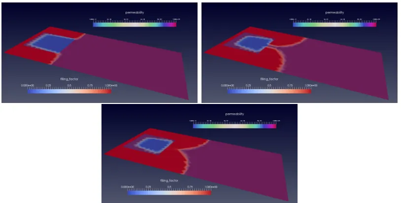
K2 K1 (see Fig. 3.1). In this case the resin can race around the low permeability region
and the front becomes discontinuous, creating a macroscopic void behind the main front as
demonstrated in Fig. 3.2. Based on the one-dimensional model (2.1) and Proposition 2.1, it
is not difficult to estimate that it is sufficient to haveK2/K1 <1/9 for appearance of a void.
Macroscopic voids are one of the main defects in composites leading to scrap and failures (see
e.g. [2] and references therein). Possible discontinuities of the front cause difficulties in both
analytical analysis of (3.1) and its numerical approximation as we discuss further in Sections4
and 5.1.
In practice one does not have a deep vacuum (i.e.,p0cannot be assumed negligible) and air
is entrapped in macrovoids [2]. To take into account air entrapment, one can replace the model
(3.1) by a two-phase model with one phase (resin) being incompressible (as it is in (3.1)) and
the other (air) being compressible. But such a model is computationally expensive, while to
Figure 3.1: The 2m by 1m rectangular domain ¯D with inlet∂DI being the left side of ¯Dand
outlet∂DO being the right side of ¯D. The top and the bottom sides of ¯D form the perfectly
sealed boundary ∂DN. The small domain with low hydraulic conductivity has the size 0.5m
by 0.5m. Here K1 = 10−7 m2/sec·Pa and K2 = 10−9 m2/sec·Pa, see further details in the
text.
Figure 3.2: Void formation. The thickness of the material is 1cm, the inlet pressure pI =
0.6M P a, the outlet pressure p0 = 0.1M P a, and the porosityκ = 0.7. The other parameters
are given in Fig. 3.1.
find an optimal design for a composite part’s production (e.g. optimal locations of vents and inlets), especially taking into account uncertainties, one needs to run model simulations very
many times. To this end a simplified model is considered [23,2], in which the air entrapment is
[image:9.612.91.498.333.539.2]including related commercial software (see, e.g. [2] and references therein). In the simplified
model it is assumed [23,2] that the pressure in a void increases according to the ideal gas law,
i.e., that pressure inside the void multiplied by its volume remains constant when the void shrinks during the filling process (we assume that temperature remains constant during the
process). In [23, 2] there is a discrete-type formulation of this model, here we give its PDE
formulation.
To describe this modification of (3.1), assume that at timet≥0 there are`(t) entrapments
with closed boundaries Γi(t) and volumesvi(t) formed at timesτi, i= 1, . . . , `(t),behind the
main front Γ0(t).Then we can write the model as
−∇K(x, y)∇p= 0,(x, y)∈Dt, t >0,
(3.2)
p(0, x, y) =p0, (x, y)∈D,
p(t, x, y) =pI, (x, y)∈∂DI, t≥0,
ˆ
n(x, y)· ∇p(t, x, y) = 0, (x, y)∈∂DN, t≥0,
Vi(t, x, y) =−
K(x, y)
κ nˆi(t, x, y)· ∇p(t, x, y), (x, y)∈Γi(t), i= 0, . . . , `(t), t≥0,
Γ0(0) =∂DI,
p(t, x, y) =p0, (x, y)∈Γ0(t), t >0,
p(t, x, y) =p0, (x, y)∈∂DO, t≥0,
p(t, x, y) = p0vi(τi)
vi(t)
, (x, y)∈Γi(t), t >0,
whereVi(t, x, y) are the velocities of the moving boundaries Γi(t) in the normal direction and
ˆ
n(x, y) and ˆni(t, x, y) are the unit normals to the corresponding boundaries, Dt ∈ D is the
time-dependent domain bounded by Γi(t), i = 0, . . . , `(t), and the appropriate parts of ∂D,
the rest of the notation is as in (3.1). The volumevi(t) of a void is computed as
vi(t) =H
Z
Γi(t)
dΓi(t),
whereH is a fixed thickness of the material, which is assumed to be small so that flow through
thickness can be neglected, i.e., that the two-dimensional model is a good approximation for the three dimensional flow.
It is clear that in the model (3.2) once a void is formed atτi, its volumevi(t) remains larger
than or equal to p0vi(τi)/pI and, consequently, the number of voids `(t) is a non-decreasing
function. Hence we have the following inequalities for a void’s volume:
(3.3) p0
pI
vi(τi)≤vi(t)≤vi(τi), t≥τi,
and for the void content at a fixed timeT:
p0
pI `(T) X
i=0
vi(τi)≤ `(T) X
i=0
vi(T)≤ `(T) X
i=0
vi(τi).
In the case of constant hydraulic conductivity, K(x) = K, (such a problem often called the Hele-Shaw problem or the quasi-stationary Stefan problem) existence and uniqueness of
(3.1) have been established both locally and globally and in the classical and weak senses,
see [12, 36, 15,6,9, 52] and also references therein. Note that in this case no voids can be
formed and (3.1) and (3.2) coincide. The models (3.1) and (3.2) with non-constant K(x)
can have singular-type behavior when voids form and, in the case of (3.1), also when they
collapse. Since there is no collapse of voids in (3.2), behavior of its solutions is less singular
than for (3.1) and in this sense (3.2) can be viewed as a regularization of (3.1). We are not
aware that questions concerning existence and uniqueness of solutions to (3.1) and (3.2) have
been considered in the literature, and they are an interesting and important topic for further study, especially taking into account wide use of such models in applicable sciences. Local
existence and uniqueness of solutions to (3.1) and (3.2) can potentially be addressed under
some regularity of the data similarly to [33,34].
In most cases of practical interest permeability k(x, y) (and hence the hydraulic
conduc-tivity K(x, y)) is anisotropic [8, 30, 39, 18, 24, 26]. Consequently, it is important to model
the hydraulic conductivity K(x, y) as a random tensor. The principal-axis transformation of
the hydraulic conductivity tensor gives
(3.4) K(x, y) =T(x, y)
Kxx(x, y) 0
0 Kyy(x, y)
T|(x, y),
whereT(x, y) is the rotation matrix
T(x, y) =
cosθ(x, y) sinθ(x, y) −sinθ(x, y) cosθ(x, y)
.
We assume that Kxx(x, y) = Kxx(x, y;ω) and Kyy(x, y) = Kyy(x, y;ω) can be modeled
as independent log-normal random fields and the angleθ(x, y) =θ(x, y;ω) is a Gaussian field
independent of Kxx(x, y) and Kyy(x, y). We propose that the means of Kxx(x, y), Kyy(x, y)
and θ(x, y) correspond to the hydraulic conductivity intended by the design of a composite
part and the perturbation of these means are stationary random fields modeling uncertainty
arising during the manufacturing process. Properties of the model (3.2), (3.4) are discussed
in Section 5 below based on its simulation by the CV/FEM algorithm described in the next
section.
4. Numerical algorithm. In this section, for completeness of exposition, we give an im-plementation of the interface-tracking control volume finite element method (CV/FEM) with
a fixed grid [2, 20, 45], in a form suitable for the considered stochastic model (3.2), (3.4).
CV/FEM is a volume-of-fluids technique [20,43]. It is widely used in the simulation of the
RTM filling process [2,23,5,32]. There are a number of alternatives to CV/FEM, including
level set methods [38], other volume-of-fluids methods [43], marker particle methods (see [38]
and references therein), and boundary element methods (see e.g. [53] and references therein).
Fixed-grid CV/FEM is currently the method of choice in the RTM community due to its
com-putational efficiency [2] and we follow this common RTM practice here. At the same time, it
CVi CVj
xi xj
(a) CVi contains two subelements from the bottom layer and one from the top layer.
CVi CVj
xi xj
[image:12.612.166.482.103.261.2](b) CVi contains two subelements from the bottom layer and another two from the top layer.
Figure 4.1: Two examples of tessellation of the spatial domain and the corresponding control volume subdivisions.
Let us turn to the CV/FEM description. The whole computational domain (an empty mold) is first discretized using triangular elements, and then each element is further divided into three sub-volumes by connecting the center point and the midpoints of the edges of triangle. Each node is surrounded by a control volume that is composed of all of the sub-volumes associated with that node. Note that the number of control sub-volumes is equal to the total number of nodes.
Figure 4.1 shows two different types of tessellation of the spatial domain and the
corre-sponding control volume subdivisions. Suppose that the two horizontal layers divided by a
thick line in the middle domain as in Fig. 4.1 have two different permeability values. It is
not difficult to see (and was checked experimentally) that in the case of the discretization
as in Fig. 4.1(a) the exchange of permeability values between the two layers can result in
different filling times due to the discretization asymmetry: the control volumeCVi, which has
a boundary edge, has two subelements from the bottom layer and one from the top layer. In order to avoid this bias, we choose unbiased (i.e. symmetric) control volumes as shown in
Fig.4.1(b) for our numerical experiments.
In the CV/FEM, to track the interface, a scalar parameter, fi, called the fill factor, is
assigned to each control volumeCVi. The fill factor represents the ratio of the volume of fluid
to the total volume of the control volume. The fill factorfi takes values from 0 to 1: fi = 1
for saturated region, fi = 0 for an empty region and 0 < fi <1 for a partially filled region.
If 0 ≤ fi < 1, we will say that the control volume is unsaturated. The flow front can be
reconstructed based on the nodes that have partially filled control volumes, i.e., those with 0< fi <1 (see e.g. [20,3]). In this paper we are not interested in reconstruction of the front
and hence we do not consider it here. Finding all parts of the unsaturated regions requires a
void detection algorithm. Such an algorithm was introduced in [23] and here we present its
implementation. For simplicity, we assume that there is a single vent in the mold but it is not difficult to generalize the algorithm to the case of many vents.
f1(1) f2(1) f3(0)
f4(1) f5(1) f6(0)
f7(1) f8(1) f9(1)
f10(0) f11(0)
f12(1) f13(0.5)
(a) The fill factors of 13 control volumes. Note that
CV3, CV6, andCV9 are the control volumes containing
nodes on the vent.
from vent[i]
i
3 6 0 0 0 · · · 0 1 2 3 4 5 · · · 13
iter last iter
(b) Add vent control volumesCV3 andCV6
into the array from vent, asf3<1 andf6<
1.
from vent[i]
i
3 6 11 0 0 · · · 0 1 2 3 4 5 · · · 13
iter last iter
(c) Add an unsaturated neighbour of CV3,
which is CV11 in this case, into the array
from vent and advancelast iter to the next element.
from vent[i]
i
3 6 11 13 0 · · · 0
1 2 3 4 5 · · · 13
iter last iter
(d) First advance iter to the next element. Then add an unsaturated neighbour ofCV6
into the array from vent and advance the
last iter to the next element.
from vent[i]
i
3 6 11 13 0 · · · 0
1 2 3 4 5 · · · 13
iter last iter
(e) Advanceiter to the next element. There is no unsaturated neighbour ofCV11.
from vent[i]
i
3 6 11 13 0 · · · 0
1 2 3 4 5 · · · 13
iter last iter
(f) Advanceiterto the next element. There is no unsaturated neighbour ofCV13.
from vent[i]
i
3 6 11 13 0 · · · 0
1 2 3 4 5 · · · 13
iter last iter
(g) Advance iter to the next element. Now
[image:13.612.185.402.97.258.2]iter >last iter.
Figure 4.2: An example of a process to find all unsaturated control volumes connected to the vent through unfilled control volumes.
connected to a vent. To determine which control volumes belong to voids, we first find all unsaturated control volumes which are connected to the vent (i.e., which are not voids) through unsaturated control volumes. To do this, we introduce an array of size equal to the
number of nodes, from vent and two pointers,iter and last iter, pointing at the first element
and the last nonzero element of the array, respectively. This process is done in four steps (see
Algorithm 4.1), and Figure4.2 illustrates it with an example.
Algorithm 4.1 Detection of control volumes which are connected to the vent
Step 1 Add all unsaturated control volumes where the vent is located into the arrayfrom vent,
and set two pointersiter and last iter (Figure4.2(b)).
Step 2 The loop is carried out over the neighbors of a control volumeCVi pointed at by the
pointeriterto detect first visited neighbors whose fill factors are less than 1. Each time
the neighbor is chosen to be added to from vent, move last iter to the next element
(Figure4.2(c)).
Step 3 After all neighbors ofCVi are checked, advance iter to the next element (Figure 4.2
(d)).
Step 4 RepeatStep 2 and Step 3 untiliter >last iter (Figure4.2(g)).
Now the void control volumes are all unsaturated control volumes that do not belong
to the from vent formed by Algorithm 4.1. If there are void control volumes at the current
time step tk, then each individual void is represented by a connected set of void control
volumes. Starting from any of the void control volumes, CVi, a search process (analogous to
Algorithm4.1) is used to find all void control volumes connected to CVi through void control
volumes. The total volume of each voidj is computed during the search. If the void is formed
for the first time at the time tk then we store its volume in ¯vj∗; otherwise, assign it to ¯vj(tk).
Then the pressure value, ¯pvoidj(tk), in each void (including its boundary) at the time tk is
determined using the ideal gas law as in (3.2):
(4.1) p¯voidj(tk) =
p0¯v∗j
¯
vj(tk) .
At each time steptkof the CV/FEM, the fully-saturated control volumes form the solution
domain and the finite element method is used to approximate the pressure field ¯pin the solution
domain. The corresponding boundary conditions on the inlet ∂DI and the perfectly sealed
boundary ∂DN are imposed. Further, the pressure on the outlet ∂DO and in all-partially
filled or empty control volumes not belonging to voids is set to p0 while the pressure inside
voids (i.e., for all unsaturated control volumes belonging to the voids) is set to p0 if the void
is formed at this time step and to ¯pvoidj(tk) otherwise.
After computing the approximate pressure field ¯p, we calculate the velocity field for
com-pletely filled control volumes adjacent to unsaturated control volumes at the centroid of each element using the Darcy’s law:
(4.2) u(t, x, y) =−K(x, y)· ∇p¯(t, x, y)
κ ,
whereu is the superficial fluid velocity.
x
1x
2x
3a
b
c
o
~u
e j
~n
1~n
2 [image:15.612.183.402.96.265.2]~n
3Figure 4.3: Calculation of the local flow rate on a triangular elementej with nodes x1, x2, x3.
Assuming that the fluid velocity is constant throughout each element, we compute the local
flux into each subelement. Figure 4.3 illustrates the local flux calculation in the triangular
elementei. The midpoints of the three sides ofei are denoted asa,b, andcand pointois the
center of the element. The vectors ~n1,~n2, and ~n3 are unit normal vectors perpendicular to
the surfaces oa,ob, andoc, respectively. The local flux into each subelement associated with
a nodexi in element ej,Qej,xi,i= 1,2,3, is calculated as
Qej,x1 =−uej·(~n1|oa| −~n3|oc|)H, Qej,x2 =−uej·(~n2|ob| −~n1|oa|)H,
(4.3)
Qej,x3 =−uej ·(~n3|oc| −~n2|ob|)H,
where H is the thickness of the mold. The total fluxes entering into the control volume CVi
is then calculated by assembling the local fluxes:
(4.4) Qi =
X
el∈Ei
Qel,xi,
whereEi is the set of elements containing the nodexi.
Having computed all the fluxes, we calculate the new fill factor fi(tk+1) =fi(tk+δt) of
the unsaturated control volume ias
(4.5) fi(tk+δtk) =fi(t) +
δtkQi(t)
Vi ,
where Vi is the volume of control volume i. The time increment δtk is calculated so that at
least one control volume is filled during the current time step and
(4.6) δtk= min
i
(1−fi(tk))Vi Qi
,
front) at time tk. Note that the element on which the minimum is reached becomes filled at tk+1=tk+δtk.
This simulation process continues for every time step until one of two conditions is met: either (1) the entire mold is filled or (2) there is an equilibrium of pressure between the interior and the exterior of all voids and the rest of the mold is filled. The corresponding
timeτh is considered as the approximate filling time obtained with the mesh size h (h is the
length of hypotenuse of the triangular element). To summarize, the CV/FEM is presented in
Algorithm 4.2.
Algorithm 4.2 Control volume finite element method (CV/FEM)
Step 1. Create control volumes. Set t0 = 0 and k= 0.
Step 2. Identify the saturated domain by the fill factors and detect void control volumes
using Algorithm 4.1.
Step3. Compute the pressure field ¯pin the saturated domain with the appropriate boundary
conditions by the FEM.
Step 4. Calculate the pressure gradients, ∇p¯, in the neighborhood of the flow front by
differentiating the element shape functions and then compute the velocity field, u, using
Darcy’s law (4.2).
Step 5. Calculate the volumetric flow rate, Q, as in (4.3) and (4.4).
Step 6. Find the size of the time step δtk by (4.6).
Step 7. Update the fill factors with (4.5) and advance the time: tk+1 = tk+δtk and set
k=k+ 1.
Step 8. Repeat fromStep 2 for the newly-filled domain until the mold is completely
satu-rated or there is an equilibrium of pressure between the interior and the exterior of all voids and the rest of the mold is filled.
To simulate the stochastic model (3.2), (3.4), we need to generate the random hydraulic
conductivity tensor K(x, y) at the centers of triangular elements, which requires to sample
from stationary Gaussian distributions according to the proposed stochastic model forK(x, y)
at the end of Section 3. To generate the required Gaussian random fields, we exploit the
block circulant embedding method from [31], which is an extension of the classical circulant
embedding method [11,46] from regular grids to block-regular grids.
5. Numerical experiments. In this section, we present results of numerical experiments
which aim at (i) examining convergence of Algorithm 4.2for the model (3.2) with the
quan-tities of interest being the filling time and void content (Section 5.1); and (ii) studying how
variability of permeability affects the filling time in the RTM process (Sections5.2-5.4). To
ex-perimentally study convergence in Section 5.1, we use the deterministic version of the model
(3.2), i.e., when the hydraulic conductivity K(x, y) is a given deterministic tensor. In the
stochastic experiments in Sections5.2-5.4we consider the model (3.2), (3.4) with various
pa-rameters of the random hydraulic conductivity K(x, y). The principal conductivity values,
Kxx and Kyy, and the angle θ(x, y) are assumed to be independent stationary random fields,
withKxxand Kyy being log-normal andθ(x, y) being Gaussian. In our experiments the three
Mat´ern covariance functions (2.15)-(2.17) for the Gaussian random fields logKα,α=xx, yy,
Inlet Outlet 20cm
[image:17.612.120.468.107.285.2]10cm
Figure 5.1: Schematic illustration of the mold geometry with an inlet gate and an outlet gate and tessellation of the spatial domain.
and θ, are used with the following scaled distance
(5.1) d(x, λ) =
s
x2
x λx
2
+
x2
y λy
2
,x= (xx,xy).
In Sections 5.2-5.4 we will denote the means of Kxx, Kyy and θ by µKxx, µKyy and µθ,
respectively, and the standard deviations ofKxx,KyyandθbyσKxx,σKyy andσθ, respectively.
In each particular experiment the covariance function and the correlation lengths λx and λy
will be chosen to be the same for all three random fields. To compute expectation and variance
of the filling time τ, we exploit the Monte Carlo technique using 3000 independent runs of
(3.2), (3.4) in all the Monte Carlo experiments presented in Sections 5.2-5.4.
In all our experiments the resin is injected into a rectangular mold of size 20cm×10cm
×0.1cm as shown in Figure 5.1. The horizontal direction is viewed as the x-direction and
vertical as they-direction. Since in this work we assume that there is no flow in the thickness
direction, we use two-dimensional elements for modeling the flow. In what follows we denote
the mesh size byh, which is the length of hypotenuse of the triangular element. The physical
properties of the preform are chosen in all the experiments, except the ones with a void in
Section5.1, as listed in Table 5.1.
5.1. Convergence of the CV/FEM. In this section we deal with the deterministic version
of the model (3.2), i.e., when the hydraulic conductivityK(x, y) is a given deterministic tensor.
We apply Algorithm4.2 to this model and examine its convergence looking at two quantities
of interest: the filling time τ (it is not random in this experiment, of course) and volume of a
Porosity κ= 0.7
Injection pressure pI = 0.6 MPa
[image:18.612.203.382.94.138.2]Vent pressure p0 = 0.1 MPa
Table 5.1: Physical properties of the preform.
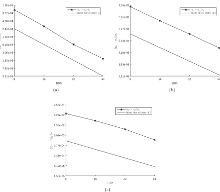
To estimate the error of the simulated filling time τh obtained with the mesh size h,
we use a reference solution τh∗ obtained on a grid with the small mesh size h∗ = 10/128
cm. Three different shapes of the flow front determined by different choices of the hydraulic
conductivityK(x, y) tensor are considered: (a) straight line parallel to y-axis (Kxx =Kyy =
10−8 m2/sec·Pa); (b) cup-shaped front (K
xx(x, y) = 10−9+ 10−8(1−sin(πy/0.1)) m2/sec·Pa,
Kyy = 10−10 m2/sec·Pa); and (c) cap-shaped front (Kxx(x, y) = 10−9 + 10−8sin(πy/0.1)
m2/sec·Pa, K
yy= 10−10m2/sec·Pa). The convergence of the resin filling timeτh with respect
to the mesh resolution h is shown in Fig. 5.2. We observe that |τh∗ −τh|/τh∗ converges
approximately quadratically in all three cases. At the same time, we see that the geometry of the flow front has an influence on the accuracy. The most accurate results are seen in the
case of the flat flow front (Figure 5.2(a)) and the least accurate results are seen in the case
of the cap-shaped front (Figure 5.2(c)).
Void formation in RTM processes has received considerable interest due to its effect on
the degradation of physical and mechanical properties of the composite. According to [21,19],
even a void content of just 1% can substantially affect mechanical properties of the material, e.g., decrease of strength up to 30% in bending, 9% in torsional shear, 8% in impact, etc. Consequently, we view that it is important to look at convergence of the CV/FEM for the void content, despite not considering void formation in further experiments here.
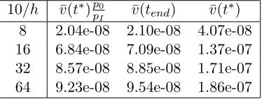
Let us look at accuracy of the CV/FEM with presence of a void. In order to have a
void in the solution of (3.2), we incorporate a low permeability patch (1cm ≤x ≤3cm and
4cm ≤ y ≤ 6cm), where the permeability value is 100 times lower than that of the rest of
the mold, 10−7 m2/sec·Pa (see also the corresponding discussion in Section3). In this setting
only a single void can form. We look at the void volume ¯v(t) at the timet∗ when it is formed
and at the timetend when the mold is fully saturated except the void.
10/h ¯v(t∗)p0
pI v¯(tend) v¯(t
∗)
8 2.04e-08 2.10e-08 4.07e-08
16 6.84e-08 7.09e-08 1.37e-07
32 8.57e-08 8.85e-08 1.71e-07
[image:18.612.201.388.532.603.2]64 9.23e-08 9.54e-08 1.86e-07
Table 5.2: The volume of void (inm3) at t∗ and t
end and also the lower bound for ¯v(tend) as
in (3.3). Here pI = 0.6 MPa and p0 = 0.3 MPa.
Table5.2 shows that the inequality (3.3) holds in the discrete case. The volumes of void
at two times,t∗ andt
end, are both increasing as the mesh size h becomes smaller. Two plots
10/h
8 16 32 64
| τh 8 − τh | / τh ∗ 3.81e-06 7.63e-06 1.53e-05 3.05e-05 6.10e-05 1.22e-04 2.44e-04 4.88e-04 9.77e-04 1.95e-03
|τh∗−τh|/τh∗
linear line of slope -2
(a)
10/h
8 16 32 64
| τh 8 − τh | / τh ∗ 3.81e-06 1.53e-05 6.10e-05 2.44e-04 9.77e-04 3.91e-03 1.56e-02
|τh∗−τh|/τh∗
linear line of slope -2.3
(b)
10/h
8 16 32 64
| τh 8 − τh | / τh ∗ 1.53e-05 6.10e-05 2.44e-04 9.77e-04 3.91e-03 1.56e-02 6.25e-02 2.50e-01
|τh∗−τh|/τh∗
linear line of slope -1.7
[image:19.612.76.521.109.498.2](c)
Figure 5.2: The error of the filling time |τh∗ −τh|/τh∗ depending on the shapes of the flow
front: (a) flat flow front, (b) cup-shaped flow front, and (c) cap-shaped flow front.
in Fig. 5.3show that the volume of void converges with approximately first order in h.
To conclude, we experimentally observed approximately 2nd order convergence of the
CV/FEM Algorithm4.2 for the filling time and a lower order, approximately 1st order,
con-vergence for the volume of void.
5.2. Pseudo-1D flow. Now we consider the model (3.2), (3.4) with relatively high mean
horizontal conductivity µKxx and low mean vertical conductivity µKyy (i.e., µKxx >> µKyy),
which results in limited movement of flow in the vertical direction. We also choose the
10/h
8 16 32
| ¯ vh ( t ∗) −
¯vh/
2 ( t ∗) | 1.1e-08 1.5e-08 2.1e-08 3.0e-08 4.2e-08 6.0e-08 8.4e-08 1.2e-07
|¯vh(t∗)−¯vh/2(t∗)|
linear line of slope -1.2
(a)
10/h
8 16 32
| ¯ vh ( ten d ) − ¯
vh/
2 ( ten d ) | 5.3e-09 7.5e-09 1.1e-08 1.5e-08 2.1e-08 3.0e-08 4.2e-08 6.0e-08
|¯vh(tend)−¯vh/2(tend)|
linear line of slope -1.4
[image:20.612.74.529.115.299.2](b)
Figure 5.3: Void size difference between two consecutive discretization levels (a) at time t∗
when the void is formed for the first time and (b) at time tend when the mold is completely
filled except the void.
λx>> λy). The parameters of the random conductivity tensorK(x, y) used in this subsection
are listed in Table5.3. We conduct 9 separate numerical experiments using the 3 different
val-ues ofλxfor each of the three different Mat´ern covariance functions with different smoothness
ν.
µKxx 1e-8m
2/sec·Pa µ
θ 0 radian
σKxx 8e-9m
2/sec·Pa σ
θ 0.0356 radian
µKyy 1e-9m
2/sec·Pa λ
x 0.01m, 0.03m, 0.05 m
σKyy 8e-10m
2/sec·Pa λ
y 0.001m
Table 5.3: The parameters for the random hydraulic conductivity tensorK(x, y) used in the
pseudo-1D flow simulation.
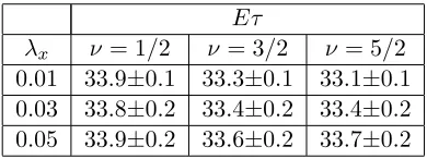
The results of the experiments are presented in Tables 5.4 and 5.5. We observe that
the mean filling time Eτ shows almost no dependence on either the horizontal correlation
length λx or on smoothness ν of the random hydraulic conductivity field K(x, y), while the
variance of the filling time increases with increase ofλx and ν. This is consistent with the 1D
flow properties studied in Section 2 and one can conclude that when µKxx >> µKyy, a good
qualitative prediction about the filling time τ can be made using the analytically solvable
one-dimensional problem (2.1). Note that the filling time according to the design here and in
the corresponding one-dimensional case (see Section 2) coincide as expected but it is not so
forEτ (see Remark5.1below). We also plot typical sample densities forτ (see Fig. 5.4). We
observe that the probability of filling timeτ being in a range close to the designed time (2.8
[image:20.612.162.429.439.496.2]t
5 10 15 20 25 30 35 40 45 50
0 0.02 0.04 0.06 0.08 0.1 0.12 0.14 0.16 0.18
t
0 5 10 15 20 25 30 35 40 45 50
0 0.02 0.04 0.06 0.08 0.1 0.12 0.14 0.16
t
0 10 20 30 40 50 60
0 0.01 0.02 0.03 0.04 0.05 0.06 0.07 0.08 0.09 0.1
t
0 10 20 30 40 50 60
[image:21.612.107.480.102.395.2]0 0.01 0.02 0.03 0.04 0.05 0.06 0.07 0.08 0.09 0.1
Figure 5.4: Sample densities forτ (in sec) in the case of pseudo-1D flow. The left top figure:
ν = 1/2, λ = 0.01; the right top figure: ν = 5/2, λ = 0.01; left bottom figure: ν = 1/2,
λ= 0.05; right bottom figure: ν= 5/2,λ= 0.05.
sec here) is very low.
Eτ
λx ν = 1/2 ν = 3/2 ν= 5/2
0.01 33.9±0.1 33.3±0.1 33.1±0.1
0.03 33.8±0.2 33.4±0.2 33.4±0.2
0.05 33.9±0.2 33.6±0.2 33.7±0.2
Table 5.4: Mean filling time Eτ (in sec) and its 95% confidence interval for the pseudo-1D
flow. The filling time according to the design is equal to 2.8 sec.
[image:21.612.196.391.501.574.2]mean filling times in 1D and 2D cases can be illustrated in the following way. Let us imagine the extreme case of the pseudo-1D flow so that Kyy=0 and θ = 0. Suppose in our domain
discretization we have l horizonal strips via which resin is propagating. Each strip has its own time-to-fill τi on each realization of the random field K(x). Then for τ = max1≤i≤lτi
we have Eτ ≥ Eτi. It is an interesting probabilistic mini-problem to study the relationship
between τ and τi, in particular betweenEτ and Eτi, as well as the limiting case l → ∞, but
we do not consider it here. We emphasize that in the deterministic case with Kxx >> Kyy
the one-dimensional model gives good predictions for the two-dimensional model and, being considerably simpler, it is often used in practice for this purpose. However, here we highlight that in the stochastic case there are considerable quantitative differences between statistical characteristics of the pseudo-1D flow and the 1D flow despite the fact that qualitatively they are similar. This observation is important from the practical point of view. Further, in [22, 50] expansions of moments of the interface dynamics were derived using a dynamical mapping of the Cartesian coordinate system onto a coordinate system associated with the moving front. Making use of the ideas of [22] to obtain expansions for variance of filling times is an interesting problem (even if we assume that discontinuity of the front due to possible void formation can be neglected) for future research.
Varτ
λx ν = 1/2 ν = 3/2 ν= 5/2
0.01 12.9±1.5 13.5±1.8 15.3±1.9
0.03 18.8±1.5 20.0±1.6 20.4±1.5
[image:22.612.198.391.342.416.2]0.05 22.7±1.7 26.2±2.0 28.4±2.2
Table 5.5: Variance of the filling time Varτ (in sec2) and its 95% confidence interval for the
pseudo-1D flow.
5.3. Two-dimensional isotropic flow. The second stochastic numerical experiment uses
the following parameters of the random hydraulic conductivity: µKxx=µKyy = 1e-8m
2/sec·
Pa, σKxx = σKyy = 8e-9m
2/sec·Pa, µ
θ = 0, σθ = 0.0356 radians, and λx = λy = {0.01m,
0.03m, 0.05m}. The focus of this experiment is again to investigate the impact of the
corre-lation length and smoothness of the random field K(x, y) on the filling time.
Eτ
λx=λy ν = 1/2 ν= 3/2 ν = 5/2
0.01 37.8±0.2 39.4±0.2 39.8±0.2
0.03 42.1±0.5 43.6±0.5 43.3±0.5
0.05 43.3±0.6 45.2±0.7 45.4±0.7
Table 5.6: Mean filling time Eτ (in sec) and its 95% confidence interval for the 2D isotropic
flow. The filling time according to the design is equal to 2.8 sec.
[image:22.612.188.400.559.631.2]Varτ
λx=λy ν = 1/2 ν= 3/2 ν = 5/2
0.01 32.4±2.6 35.1±2.5 35.4±2.4
0.03 170±12 216±17 219±20
[image:23.612.189.399.95.168.2]0.05 300±23 432±41 424±41
Table 5.7: Variance of the filling time Varτ (in sec2) and its 95% confidence interval for the
2D mean isotropic flow.
Unlike the pseudo-1D results presented in Section 5.2, where the mean filling time Eτ is
independent of the correlation length and smoothness, here Eτ increases with growth of the
correlation length as shown in Table 5.6 and slightly grows with increase of smoothness. In
other words, 2D flow moves slower on a more homogeneous porous medium with less spatial
variability than in the pseudo-1D case. We also observe a fast increase of variance Varτ with
an increasing spatial correlation length in Table5.7.
5.4. Two-dimensional flow with anisotropic mean. The third stochastic numerical
ex-periment uses the following parameters of the random hydraulic conductivity: µKxx = 1e
-8m2/sec·Pa, µ
Kyy = 2e-8m
2/sec·Pa, σ
Kxx = σKyy = 8e-9m
2/sec·Pa, µ
θ = 0, σθ = 0.0356
radian, and λx = λy = {0.01m, 0.03m, 0.05m}. In other words, here (in comparison with
Section5.3) we consider a model in which random hydraulic conductivity has an anisotropic
mean. Recall (see Section 3) that we proposed that the means of Kxx(x, y), Kyy(x, y) and
θ(x, y) correspond to the hydraulic conductivity intended by the design of a composite part
and that in most cases of practical interest permeability k(x, y) (and hence the hydraulic
conductivity K(x, y)) is anisotropic by design. Note that the mean of permeability in the
x-direction (Kxx) is smaller than that in they-direction (Kyy) and that the 1D model from
Section2 does not apply here (see the discussion in Section5.2).
The results of the numerical experiments are presented in Tables 5.8and5.9. We observe
that the mean filling time Eτ of the 2D mean anisotropic flow increases as the correlation
length increases and also that an increasing spatial correlation length leads to an increase of Varτ.
Eτ
λx=λy ν = 1/2 ν= 3/2 ν = 5/2
0.01 35.4±0.2 36.8±0.2 37.0±0.2
0.03 39.3±0.4 40.1±0.5 40.3±0.5
0.05 40.1±0.6 42.1±0.7 42.1±0.7
Table 5.8: Mean filling time Eτ (in sec) and its 95% confidence interval for the 2D mean
anisotropic flow. The filling time according to the design is equal to 2.64 sec.
We note that in all three stochastic cases considered in Sections 5.2-5.4 the mean
[image:23.612.187.400.532.604.2]emphasises the importance of stochastic modeling of RTM.
Varτ
λx=λy ν = 1/2 ν= 3/2 ν = 5/2
0.01 24.9±2.0 26.1±1.7 27.9±2.0
0.03 135±9 185±26 178±13
[image:24.612.189.398.118.191.2]0.05 257±23 355±33 353±27
Table 5.9: Variance of the filling time Varτ (in sec2) and its 95% confidence interval for the
2D mean anisotropic flow.
Remark 5.2. The MATLAB codes for the CV/FEM used in our experiments are available at https://github.com/parkmh/MATCVFEM.
6. Discussion and summary. In this work we considered stochastic one-dimensional and two-dimensional moving-boundary problems suitable for modeling RTM processes. The PDE formulation of the main two-dimensional model which takes into account compressible air entrapment in voids behind the main front is somewhat novel. The one-dimensional problem has an analytical solution while the two-dimensional model requires a numerical method for
computing quantities of interest. Following the common practice in the RTM community [2],
we use the control volume-finite element method (CV/FEM) to simulate the two-dimensional problem. We test accuracy of the CV/FEM algorithm for three particular cases of deter-ministic hydraulic conductivity, and we experimentally observed approximately its 2nd order convergence for the filling time and a lower order, approximately 1st order, convergence for the volume of void. We note that these tests were done in the case of infinitely smooth (in the case of the filling time) or piece-wise constant (in the case of the volume of void) hydraulic conductivity while less regular random field are used to model hydraulic conductivity. For future study, it is of interest to look at dependence of behavior of the CV/FEM algorithm on the smoothness of hydraulic conductivity and on various observables.
We studied properties of a stochastic one-dimensional moving-boundary problem with the hydraulic conductivity being modelled as a stationary log-normal random field. In particular, we observe that the mean filling time does not depend on correlation length or on smoothness of hydraulic conductivity, while the filling time variance (as a measure of its variability) does depend on both the correlation length and smoothness. A similar conclusion is made about the two-dimensional model’s behavior when random permeability in the direction from inlet to outlet is much bigger than in the perpendicular direction (the case of pseudo-1D flow). However, we discovered that in other cases of random permeability the mean filling time does depend on correlation length and on smoothness. The important consequence of these conclusions is the observed (often high) sensitivity of the mean and variance of the filling time to changes in correlation length of the permeability as well as in its smoothness. This highlights the importance of conducting laboratory experiments from which covariance of the permeability field can be reconstructed. Further, sensitivity of filling time to smoothness of permeability serves as a warning that stochastic modeling of permeability via homogenization procedures needs to be done with a very careful choice of scales.
Among the main objectives of this paper was to attract attention of the UQ community to challenges posed by stochastic moving-boundary problems, which are highly relevant to mod-ern technological processes in production of composite materials as well as to other porous media problems. The challenges include (i) establishing existence and uniqueness results for two and three dimensional moving-boundary problems of the type considered in this work; (ii) numerical analysis for the corresponding CV/FEM algorithm; (iii) development of faster
sam-pling techniques, e.g. using a multi-level Monte Carlo approach [17,27,28] and/or polynomial
chaos expansions [16, 48, 47]; (iv) computational experiments with complex geometry using
outcomes of (iii); (v) comparing the CV/FEM with other numerical approaches to moving
boundary problems, e.g. level sets methods [38]; (vi) design of laboratory experiments and
collection and analysis of the corresponding data to recover characteristics of random perme-ability and to find a stochastic model of the conductivity consistent with experimental data
(for recent research in this direction see e.g. [2, 24, 26]); and (vii) considering a two-phase
model involving both incompressible (resin) and compressible (air) phases and comparing its properties with the ones for the reduced model studied here.
Acknowledgements. This work was partially supported by the EPSRC grant EP/K031430/1. The authors are very grateful to Matthew Hubbard, Arthur Jones, Andy Long, Alex Skordos, and Kris van der Zee for useful discussions. We also express special thanks to Mikhail Matveev who read drafts of this paper and gave insightful feedbacks from the engineering prospective.
REFERENCES
[1] R.J. Adler, J.E. Taylor.Random Fields and Geometry. Springer, 2007.
[2] S.G. Advani, E.M. Sozer.Process Modeling in Composites Manufacturing. CRC Press, 2011.
[3] N. Ashgriz, J.Y. Poo. FLAIR: Flux line-segment model for advection and interface reconstruction. J.
Comput. Phys.93(1991), 449–468.
[4] T. Astrom.Manufacturing of Polymer Composites. Chapman and Hall, 1997.
[5] M.V. Bruschke, S.G. Advani. A finite element/control volume approach to mold filling in anisotropic porous media.Polymer Composites,11(1990), 398-405.
[6] X. Chen. The Hele-Shaw problem and area-preserving curve-shortening mortions.Arch. Rational Mech.
Anal.123(1993), 117–151.
[7] W. K. Chui, J. Glimm, F.M. Tangerman, A.P. Jardine, J.S. Madsen, T.M. Donnellan, R. Leek. Case study from industry: process modeling in resin transfer molding as a method to enhance product quality.SIAM Rev.39(1997), 714–727.
[8] G. Dagan.Flow and Transport in Porous Formation. Springer, 1989.
[9] K. Deckelnick, C. Elliott. Local and global existence results for anisotropic Hele-Shaw flows.Proc. Royal
Soc. Edin. Sec. A129(1999), 265–294.
[10] Design and Manufacture of Textile Composites. Edited by A.C. Long. Woodhead Publ., 2005.
[11] C.R. Dietrich, G.N. Newsam. Fast and exact simulation of stationary Gaussian processes through circulant embedding of the covariance matrix.SIAM J. Sci. Comp.18, (1997), 1088-1107.
[12] C.M. Elliot, V. Janovsky. A variational inequality approach to Hele-Shaw flow with a moving boundary.
Proc. Royal Soc. Edin. Sec. A88(1981), 93–107.
[13] A. Endruweit, A.C. Long. Influence of stochastic variations in the fibre spacing on the permeability of bi-directional textile fabrics.Composites A37(2006), 679–94.
[14] A. Endruweit, A.C. Long, F. Robitaille, C.D. Rudd. Influence of stochastic fibre angle variations on the permeability of bi-directional textile fabrics.Composites A37(2006), 122–32.
[15] J. Escher, G. Simonett. Classical solutions of multi-dimensional Hele-Shaw models.SIAM J. Math. Anal.
[16] R. Ghanem, P. Spanos.Stochastic Finite Elements: A Spectral Approach. Springer, 1991. [17] M.B. Giles. Multilevel Monte Carlo methods.Acta Numerica24(2015), 259-328.
[18] F. Gommer.Stochastic Modelling of Textile Structures for Resin Flow Analysis. PhD Thesis, University of Nottingham, Nottingham (UK), 2013.
[19] Y.K. Hamidi, L. Aktas, M.C. Altan. Formation of microscopic voids in resin transfer molded composites.
Trans. ASME 126(2004), 420–426.
[20] C.W. Hirt, B.D. Nichols. Volume of fluid (VOF) method for dynamics of free boundaries.J. Comp. Phys.
19(1981), 201–225.
[21] N.C.W. Judd, W.W. Wright. Voids and their effects on mechanical properties of composites – an appraisal.
SAMPE Q.14(1978), 10-14.
[22] Yu.N. Lazarev, P.V. Petrov, D.M. Tartakovsky. Interface dynamics in randomly heterogeneous porous media.Adv. Water Resources 28(2005), 393–403.
[23] B. Liu, S. Bickerton, S.G. Advani. Modelling and simulation of resin transfer moulding (RTM) - gate control, venting and dry spot prediction.Composites A27A(1996), 135–141.
[24] T.S. Mesogitis, A.A. Skordos, A.C. Long. Uncertainty in the manufacturing of fibrous thermosetting composites: a review.Composites A57(2014), 67–75.
[25] B. Mat´ern. Spatial Variation. Meddelanden fr¨an Statens Skogsforskningsinstitut, 49, No. 5, 1960 [2nd Edition, Lecture Notes in Statistics, No. 36, Springer, 1986].
[26] M.Y. Matveev, F. Ball, I.A. Jones, A.C. Long, P.J. Schubel, M.V. Tretyakov. Uncertainty in Automated Dry Fibre Placement (ADFP) and its effects on permeability (submitted)
[27] F. M¨uller, P. Jenny, D.W. Meyer. Multilevel Monte Carlo for two phase flow and Buckley-Leverett transport in random heterogeneous porous media.J. Comp. Phys.250(2013), 685–702.
[28] F. M¨uller, D.W. Meyer, P. Jenny. Solver-based vs. grid-based multilevel Monte Carlo for two phase flow and transport in random heterogeneous porous media.J. Comp. Phys.268(2014), 39–50.
[29] S.K. Padmanabhan, R. Pitchumani. Stochastic modelling of nonisothermal flow during resin transfer molding.Int. J. Heat Mass Trans.42(1999), 3057–3070.
[30] E.K. Paleologos, S.P. Neuman, D. Tartakovsky. Effective hydraulic conductivity of bounded, strongly heterogeneous porous media.Water Resources Research 32(1996), 1333–1341.
[31] M. Park, M.V. Tretyakov. A block circulant embedding method for simulation of stationary Gaussian random field on block-regular grids. Int. J. Uncertainty Quantification,5(2015), pp. 527–544. [32] F.R. Phelan. Simulation of the injection process in resin transfer molding.Polymer Composites,18(1997),
460–476.
[33] E.V. Radkevich. Conditions for the existence of a classical solution of a modified Stefan problem (the Gibbs-Thomson law).Russian Acad. Sci. Sb. Math.75(1993), 221–246.
[34] E.V. Radkevich, B.O. `Eshonkulov. On the existence of the classical solution of the problem of impregna-tion of glass-like polymers.Russian Acad. Sci. Dokl. Math.46(1993) 92–97.
[35] C.E. Rasmussen, C.K.I. Williams.Gaussian Processes for Machine Learning. MIT Press, 2006. [36] J.F. Rodrigues.Obstacle Problems in Mathematical Physics. Elsevier, 1987.
[37] Y. RubinApplied Stochastic Hydrogeology. Oxford University Press, 2003.
[38] J.A. Sethian. Level Set Methods and Fast Marching Methods : Evolving Interfaces in Computational
Geometry, Fluid Mechanics, Computer Vision, and Materials Science. Cambridge University Press,
1999.
[39] A.A. Skordos, M.P.F. Sutcliffe. Stochastic simulation of woven composites forming.Compos. Sci. Technol.
68(2008), 283–96.
[40] S. Sriramula, M.K. Chryssanthopoulos. Quantification of uncertainty modelling in stochastic analysis of FRP composites.Composites A40(2009), 1673–84.
[41] M.L. Stein.Interpolation of Spatial Data: Some Theory for Kriging.Springer, 1999.
[42] D.M. Tartakovsky, C.L. Winter. Dynamics of free surfaces in random porous media.SIAM J. Appl. Math.
61(2001), 1857-1876.
[43] G. Tryggvason, R. Scardovelli, S. Zaleski.Direct Numerical Simulations of Gas-Liquid Multiphase Flows. Cambridge University Press, 2011.
[44] B. Verleye, D. Nuyens, A. Walbran, M. Gan. Uncertainty quantification in liquid composite moulding processes. Proceedings of the FPCM11 Conference, 2012.
[45] V.R. Voller.Basic Control Volume Finite Element Methods for Fluids and Solids. World Scientific, 2009.
[46] A. T. A. Wood, G. Chan. Simulation of stationary Gaussian processes in [0,1]d.J. Comp. Graph. Stat.3 (1994), 409–432.
[47] D. Xiu. Numerical Methods for Stochastic Computations: A Spectral Method Approach. Princeton Uni-versity Press, 2010.
[48] D. Xiu, G.E. Karniadakis. Modeling uncertainty in flow simulations via generalized polynomial chaos.J.
Comp. Phys.187(2003), 137-167.
[49] D. Xiu, D.M. Tartakovsky. A two-scale nonperturbative approach to uncertainty analysis of diffusion in random composites.Multiscale Model. Simul.2(2004), 662–674.
[50] D. Xiu, D.M. Tartakovsky. Numerical methods for differential equations in random domains.SIAM J.
Sci. Comput.28(2006), 1167–1185.
[51] A. M. Yaglom.Correlation Theory of Stationary and Related Random Functions, vol. 1. Springer, 1987. [52] F. Yi. Global classical solution of quasi-stationary Stefan free boundary problem.App. Math. Comp.160
(2005), 797–817.
[53] N. Zabaras, S. Mukherjee. An analysis of solidification problems by the boundary element method.Int.
J. Numer. Meth. Engng.24(1987), 1879–1900.