Modeling feedbacks between a boreal forest and the planetary boundary layer

Modeling feedbacks between a boreal forest and the planetary

boundary layer

T. C. Hill,1 M. Williams,1 and J. B. Moncrieff1

Received 24 September 2007; revised 8 January 2008; accepted 22 May 2008; published 12 August 2008.

[1] The atmosphere and biosphere interact strongly in the planetary boundary layer. Understanding the mechanisms controlling the coupled atmosphere-biosphere system allows improved scaling between observations at the stand scale (e.g., flux towers) and those at larger scales, e.g., airborne or satellite measurements. Simulation of the joint atmosphere-biosphere system permits the study of feedbacks occurring within the coupled system. In this paper, two well-tested models, one a process-based biosphere model (SPA) and the other a planetary boundary layer model (CAPS), were coupled to allow simulation of atmosphere-biosphere feedbacks and interactions with a focus on ecological controls. As part of the validation process, the biosphere model was tested using eddy covariance, surface meteorology, and soil data collected during a 120 day period at a boreal black spruce site during the 1994 BOREAS field campaign. The coupled atmosphere-biosphere model was also validated with radiosonde data above the black spruce site, demonstrating that atmosphere and biosphere models can be coherently combined. We show that negative feedbacks at the black spruce site have strong moderating effects. The feedbacks reduce the mean impact of LAI changes on the atmospheric surface layer by 21% for latent energy, 64% for air temperature, and 44% for water mixing ratio. We show that both radiative and hydraulic limitations imposed by the vegetation structure strongly affected the interactions within the atmosphere-biosphere system, while the impact of the canopy roughness length was weak.

Citation: Hill, T. C., M. Williams, and J. B. Moncrieff (2008), Modeling feedbacks between a boreal forest and the planetary boundary layer,J. Geophys. Res.,113, D15122, doi:10.1029/2007JD009412.

1. Introduction

[2] Global climate is changing, with best estimates from

an ensemble of climate models suggesting a global average surface temperature increase (from 1980 to 1999 to 2090 – 2099) of 1.8 to 4.0 K [Intergovernmental Panel on Climate Change, 2007]. Large intermodel uncertainty was associated with the ensemble runs. The 5 – 95% confidence ranges on model predictions were approximately the same magnitude as the actual predicted temperature rises. The parameteriza-tion of land surface schemes and their interacparameteriza-tion with the climate system were a major cause of the uncertainty in the predictions of global climate models [Crossley et al., 2000; Desborough et al., 2001;Essery et al., 2003; Henderson-Sellers et al., 1995;Wood et al., 1998].

[3] Atmospheric processes are intrinsically linked to the

biosphere through the surface energy balance. The response of the terrestrial biosphere to climate perturbations thus causes changes in the atmosphere, which then in turn influence land surface processes and climate variability [Cox et al., 2000;Seneviratne et al., 2006]. The importance of atmosphere-biosphere feedbacks to climate change

predictions therefore needs to be better understood and simulated.

[4] Interactions of the land surface with the global climate

are simulated within General Circulations Models (GCMs) [Koster et al., 2006]. GCMs tend to implement simplified biosphere schemes to reduce computational costs. Such simplifications (e.g., empirical models of stomatal conduc-tance) make model calibration difficult, as many parameters may either not be measured or have little physical basis. More recently, Large Eddy Simulations (LES) have been performed for atmosphere-land surface interactions over small regions, on the order of 10 km. The use of LES models in conjunction with realistic vegetation models avoids many of the issues that GCMs face. Two dimen-sional LES schemes have shown good agreement with tall tower observations [Denning et al., 2003]. However, LES models suffer from other limitations. Because of their detail they incur large computational overheads, even for relatively small regions, and their initialization requires reanalysis data and thus reliance on other models.

[5] A role therefore exists for detailed, robust modeling

studies that focus on atmosphere-biosphere feedbacks, and which can be quickly and easily run to inform large-scale models of critical processes. Such models would lend themselves to feedback studies, data assimilation, inversion studies and other computationally intensive techniques. Recently there have been a number of models described 1_{School of GeoSciences and Centre for Terrestrial Carbon Dynamics,}

University of Edinburgh, Edinburgh, UK.

in the literature with such aims, but these models still tend to simplify and/or lack ecological components that relate to actual processes and observations [Alapaty and Mihailovic, 2006;Bounoua et al., 2006;Ek and Holtslag, 2004]. These simplifications can make implementation in ecological sensitivity/feedback analyses impractical.

[6] We coupled two well tested models; the

Soil-Plant-Atmosphere (SPA) biosphere model, and the Coupled Atmospheric boundary layer-Plant-Soil (CAPS) model. The resultant Coupled Atmosphere-Biosphere (CAB) model simulates energy, water and heat exchanges within the atmosphere-biosphere system, and operates at a spatial and temporal scale relevant to both ecological and atmo-spheric processes and measurements. The model formula-tion was designed to be (1) easily implemented and modified, (2) run with minimal computational cost, making its use in data assimilation and Bayesian studies feasible, and (3) parameterized using observations which are inde-pendent of those used in testing. The model was to be tested against both stand-based measurements (e.g., eddy covari-ance estimates of surface fluxes and surface meteorology) and atmospheric profile measurements (e.g., aircraft/radio-sonde measurements in the PBL).

[7] All model parameters were derived from previous

studies, and biogeochemical and biophysical processes were modeled mechanistically. This model is novel in that it links leaf, soil and eddy flux measurements at a site, and corroborates these with radiosonde measurements from the local region. Model results were not ‘‘tuned’’ using flux measurements, allowing greater confidence to be placed on the model’s prognostic abilities.

1.1. Paper Aims: Model Verification

[8] The verification of the model was performed in two

parts: (1) the off-line biosphere model was tested against stand-based data over a growing season and (2) the fully coupled CAB model was tested with both stand-based and atmospheric profile observations for a number of days. Verification and parameterization data came from the Boreal Ecosystems Atmosphere Study (BOREAS) [Ryan, 2000; Sellers et al., 1997]. BOREAS was chosen because of the comprehensive simultaneous data sets available, and the importance of atmosphere-biosphere water vapor and radi-ative interactions in the boreal region, which covers 11% of the terrestrial land surface [Bonan and Shugart, 1989].

1.2. Paper Aims: Coupled Feedback Sensitivity Analysis

[9] Once verified, we used the CAB model as part of a

sensitivity analysis to answer several questions:

[10] 1. Can we identify feedbacks between the PBL and

the biosphere, and what are their impacts on vegetation and PBL responses? We know high air temperatures and low humidity (i.e., high vapor pressure deficit) can stress the hydraulic system of the vegetation, forcing plants to close stomata to avoid damaging conductive tissue [Jones, 1992; Williams et al., 2001]. This defensive response of vegetation can reduce transpiration, resulting in further drying and heating of the atmosphere, increasing water vapor pressure deficit (VPD). This increased atmospheric demand for water places further stress on plant hydraulics, completing the

feedback. Can we assess the importance of feedbacks such as these and distinguish them from a simple driving force? [11] 2. What is the relative importance of changes to the

hydraulic, mechanical, and radiative properties of the bio-sphere to the coupled atmobio-sphere-biobio-sphere system? Simple variations within the biosphere, such as the height of a forest stand, may have complex impacts on the coupled system; for example, growth of forests changes the effective roughness length of the canopy which increases the effi-ciency of turbulent transport between biosphere and atmo-sphere. Increasing canopy cover also alters both the albedo and self-shading of the canopy, influencing both radiative transfers to the atmosphere and within the canopy. Because of the feedbacks involved, the effects of these changes on the coupled system are likely to be complex and nonlinear. We deconvolved the separate contributions of atmospheric interactions with vegetation radiation properties, hydraulics and canopy roughness, and assessed the importance of each in determining atmosphere-biosphere feedbacks.

2. Data Description

[12] Model runs were compared to eddy covariance,

meteorological, and radiosonde measurements within the BOREAS southern study area (SSA), located in Saskatch-ewan, Canada (53.9°N, 105.1°W), collected during the 1994 field campaign. The launch site for the radiosondes was Candle Lake (53.7°N 105.3°W, 503 m above seal level). The radiosondes provided the atmospheric profile measurements of temperature, water mixing ratio and wind speed used to initialize and verify the atmospheric submodel (Table 1). To the north and east of Candle Lake, black spruce (Picea mariana) was the dominant tree species, and in this region we assumed that black spruce dominated the daytime forcing of the boundary layer [Betts et al., 2001; Jarvis et al., 1997]. At the stand level, eddy flux, plant physiological and soil data sets from the southern study area old black spruce (SSA-OBS) eddy flux tower site were used to drive and test the biosphere submodel.

2.1. Stand-Based Data

[13] The biosphere model was parameterized using

meas-urements from the SSA-OBS site, with some parameters from other local old black spruce sites (Table 1). Plant capacitance and a stomatal water use efficiency parameter (i) were the only parameters not to be explicitly measured, or inferred from measurements. Theiparameter determines the maximum stomatal conductance. Leaf capacitance deter-mines the size of the plant water store that buffers stomatal closure after midday; typical values can range from 1 to 8 mol m 2MPa 1. Sensitivity analyses showed that these parameters were not critical, given the expected values and ranges from previous studies [Williams et al., 1996].

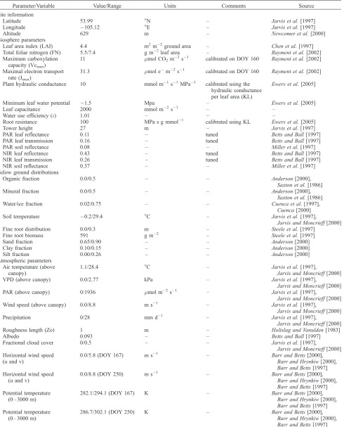
[14] The results of the biosphere model were compared to

Table 1. Model Parameters and Corroborative Dataa

Parameter/Variable Value/Range Units Comments Source

Site information

Latitude 53.99 °N – Jarvis et al.[1997]

Longitude 105.12 °E – Jarvis et al.[1997]

Altitude 629 m – Newcomer et al.[2000]

Biosphere parameters

Leaf area index (LAI) 4.4 m2_m 2_{ground area – Chen et al.[1997]} Total foliar nitrogen (FN) 5.5/7.4 g m 2leaf area – Rayment et al.[2002] Maximum carboxylation

capacity (Vcmax)

11 mmol CO2m

2

s 1 calibrated on DOY 160 Rayment et al.[2002]

Maximal electron transport rate (Jmax)

31.3 mmol e m 2s 1 calibrated on DOY 160 Rayment et al.[2002]

Plant hydraulic conductance 10 mmol m 1s 1MPa 1 calibrated using the hydraulic conductance per leaf area (KL)

Ewers et al.[2005]

Minimum leaf water potential 1.5 Mpa – Ewers et al.[2005]

Leaf capacitance 2000 mmol m 2s 1 – –

Water use efficiency (i) 1.01 – – –

Root resistance 100 MPa s g mmol 1 calibrated using KL Ewers et al.[2005]

Tower height 27 m – Jarvis et al.[1997]

PAR leaf reflectance 0.11 – tuned Betts and Ball[1997]

PAR leaf transmission 0.16 – tuned Betts and Ball[1997]

PAR soil reflectance 0.08 – – Miller et al.[1997]

NIR leaf reflectance 0.43 – tuned Betts and Ball[1997]

NIR leaf transmission 0.26 – tuned Betts and Ball[1997]

NIR soil reflectance 0.37 – – Miller et al.[1997]

Below ground distributions

Organic fraction 0.0/0.5 – – Anderson[2000],

Saxton et al.[1986]

Mineral fraction 0.0/0.5 – – Anderson[2000],

Saxton et al.[1986]

Water/ice fraction 0.02/0.75 – – Cuenca et al.[1997],

Cuenca[2000]

Soil temperature 0.2/29.4 °C – Jarvis et al.[1997],

Jarvis and Moncrieff[2000]

Fine root distribution 0.0/0.3 m – Steele et al.[1997]

Fine root biomass 591 g m 2 – Steele et al.[1997]

Sand fraction 0.65/0.90 – – Anderson[2000]

Clay fraction 0.10/0.15 – – Anderson[2000]

Silt fraction 0.00/0.26 – – Anderson[2000]

Atmospheric parameters Air temperature (above

canopy)

1.1/28.4 °C – Jarvis et al.[1997],

Jarvis and Moncrieff[2000]

VPD (above canopy) 0.0/2.77 kPa – Jarvis et al.[1997],

Jarvis and Moncrieff[2000]

PAR (above canopy) 0/1936 mmol m 2s 1 – Jarvis et al.[1997],

Jarvis and Moncrieff[2000]

Wind speed (above canopy) 0.0/8.8 m s 1 – Jarvis et al.[1997],

Jarvis and Moncrieff[2000]

Precipitation 0/28 mm d 1 – Jarvis et al.[1997],

Jarvis and Moncrieff[2000]

Roughness length (Zo) 1 m – Holtslag and Vanulden[1983]

Albedo 0.093 – – Betts and Ball[1997]

Fractional cloud cover 0/0.5 – – Jarvis et al.[1997],

Jarvis and Moncrieff[2000] Horizontal wind speed

(u and v)

0.0/5.8 (DOY 167) m s 1 _{– Barr and Betts[2000],}

Barr and Hrynkiw[2000],

Barr and Betts[1997] Horizontal wind speed

(u and v)

0.0/8.8 (DOY 250) m s 1 – Barr and Betts[2000],

Barr and Hrynkiw[2000],

Barr and Betts[1997] Potential temperature

(0 – 3000 m)

282.1/294.1 (DOY 167) K – Barr and Betts[2000],

Barr and Hrynkiw[2000],

Barr and Betts[1997] Potential temperature

(0 – 3000 m)

286.7/302.1 (DOY 250) K – Barr and Betts[2000],

Barr and Hrynkiw[2000],

[15] The eddy flux system utilized a LI-6262 (LI-COR,

Lincoln, Nebraska USA) infrared gas analyzer, and a Solent sonic anemometer (Gill Instruments Ltd, Lymington, UK) mounted on a tower 27 m above ground level. The SSA-OBS stand was 10 – 11 m in height and had an average LAI of 4.4 [Chen et al., 1997]. The tower was positioned in an extensive area of black spruce, with10% tamarack (Larix laricina). Black spruce extended from the tower at least 1200 m in all directions. Energy closure for the study period was 97%.

[16] Despite the moderately high LAI, thin crowns

resulted in significant gaps in the canopy. Under the canopy there was a sparse undergrowth of shrubs. In wetter areas Sphagnum was present, giving way to feather mosses and lichens in drier areas. The site was flat with a height variation of less than 1 m [Jarvis et al., 1997].

[17] We estimated random errors for latent energy (LE)

using half-hourly eddy flux data according to the method outlined by Hollinger and Richardson [2005]. Hollinger and Richardson suggest that errors on flux measurements follow a Laplace (double exponential) distribution, not a normal distribution. Instead of the standard deviation, the mean absolute deviation is calculated. In addition, a uniform systematic error of 20% was assumed [Goulden et al., 1996].

[18] Surface soil layers were organic (i.e., no mineral

content) [Anderson, 2000; Newcomer et al., 2000]; this necessitated some updates to the SPA model’s soil routines, which are discussed later in the description of the modeling scheme. Profiles of soil temperature [Jarvis et al., 1997; Jarvis and Moncrieff, 2000; Newcomer et al., 2000] and volumetric water content [Cuenca, 2000; Cuenca et al., 1997;Newcomer et al., 2000] were recorded at the site. Soil temperature at depths of 0.025, 0.05, 0.1, 0.2, 0.5 m were measured every half hour using thermocouples, with a reference temperature probe at a depth of 1 m. Manual volumetric water content measurements were taken period-ically (on average every 4 days) throughout the study period using a MoisturePoint manual time domain reflectometer (GS Gabel Corporation, British Columbia, Canada). Initial-izing the model with soil measurements negated the need for a ‘‘spin up’’ period.

2.2. Atmospheric Data

[19] Atmospheric profile data were taken from serial

radiosonde releases from Candle Lake [Barr and Hrynkiw, 2000;Barr and Betts, 1997, 2000;Newcomer et al., 2000]. Radiosonde releases were performed during the three BOREAS Intensive Field Campaigns of 1994. Radiosonde

data were available on 56 days throughout the 120 day study period. Release times from the Candle Lake site were typically 1115, 1515, 1715, 1915, 2115 and 2315 UTC; correcting for local time sets these times back 7 h. The site was situated 1.5 km south of Candle Lake which is 17 km long and, at widest, is 12 km wide; maps are shown byBarr et al.[1997]. The release site was a clearing 200 m wide surrounded by a mixed forest 12 – 15 m in height. To the north and east of the release site the vegetation was dominated by black spruce. However, the area immediately surrounding the launch site was not representative of the rest of the region. Thus, low-altitude radiosonde measure-ments were a reflection of the land cover at the radiosonde launch site, not the region as a whole.

2.3. Test Days

[20] The coupled atmosphere-biosphere (CAB) model

was corroborated on four test days under conditions that maximized representativeness and continuity of the data. These test days were selected from the 120 day study period using a number of criteria:

[21] 1. A minimum of two morning and two afternoon

radiosonde profiles must be available for the day in ques-tion. The first profile should be as close to dawn as possible. [22] 2. The radiosonde flight paths must remain over

black spruce dominated forest for the first 3500 m of their accent.

[23] 3. Radiosonde flight paths must not diverge by more

than a total of 45°for the first 3500 m of their accent. [24] 4. Eddy flux data should exist for the day, with no

more than 15% of the half-hourly measurements missing. [25] 5. Days should be chosen to be within periods of

stable synoptic weather conditions, in order to avoid fronts disturbing the boundary layer profiles.

[26] The suitable days based on these criteria were days

167 (16 June), 211 (30 July), 250 (7 September) and 260 (17 September).

3. Model Structure

[27] The CAB model was based on two existing models

(Figure 1). Biosphere processes and PBL processes are simulated in separate, well tested models. The biosphere component partitions the surface energy balance, calculat-ing surface evaporation, transpiration and albedo. On the basis of these parameters, the atmospheric component determines the evolution of the boundary layer. The atmo-spheric component then predicts the required meteorologi-cal drivers: temperature, VPD, downwelling radiation and wind speed, which are then passed back to the biosphere Table 1. (continued)

Parameter/Variable Value/Range Units Comments Source

Mixing ratio (0 – 3000 m) 1.0/5.4 (DOY 167) g kg 1 _{– Barr and Betts[2000],}

Barr and Hrynkiw[2000],

Barr and Betts[1997] Mixing ratio (0 – 3000 m) 4.7/6.9 (DOY 250) g kg 1 – Barr and Betts[2000],

Barr and Hrynkiw[2000],

model. Meteorological drivers are taken from the first atmospheric model layer above the forest canopy. A linear relationship is used to estimate the photosynthetically active radiation (PAR) from the shortwave radiation. The base time step for the CAB model was set at 1 min.

3.1. Ecosystem Submodel

[28] The Soil-Plant-Atmosphere (SPA) ecosystem model

[Williams et al., 1996, 2001] is a high-resolution process-based model (10 canopy layers and 20 soil layers). The model scales up from leaf-level and soil processes and measurements to landscape scales, to provide the surface fluxes and surface partitioning of energy. The SPA model is used in place of the original CAPS land surface formulation because it is based on ecological parameters that can readily be parameterized from field measurements and because the model has a history of successful corroboration by eddy flux data [Engel et al., 2002;Fisher et al., 2006;Schwarz et al., 2004;van Wijk et al., 2003;Williams et al., 1996, 1997, 2000]. In this study SPA was modified to run on a variable time step. Brief descriptions of the key features of the model are presented here.

[29] The SPA model contains a detailed radiative transfer

scheme which accounts for shaded and sunlit fractions of the canopy; simulating the absorption, transmission and reflectance of near infrared (NIR), direct and diffuse PAR and longwave radiation. Albedo is calculated on the basis of the reflectance and transmission in the PAR and NIR wavelengths of the soil and canopy elements. Canopy reflectance and transmission were derived using NIR and PAR understory reflectance [Miller et al., 1997] and

above-canopy albedos [Betts and Ball, 1997]. The canopy wind speed profile is modeled with an exponential reduction function that decreases with height [Cionco, 1985].

[30] The Farquhar model of leaf level photosynthesis

[Farquhar and Craemmerer, 1982] and the Penman-Monteith model of leaf transpiration [Jones, 1992;Monteith, 1965; Penman, 1948] are linked in the SPA model. SPA regulates stomatal conductance to maintain the minimum leaf water potential above a safe threshold to avoid exces-sive water stresses which can cause cavitation in the xylem. Plant hydraulic resistance is assumed to increase with height, increasing the potential water stress in the upper layers of the canopy and in taller canopies.

[31] Soil hydrology and temperature were calculated by

solving the soil surface energy balance and by the modeling of heat and moisture transport within 20 soil layers. Soil temperatures, water fractions and rooting profiles were initialized from measurements (Table 1). The core soil temperature was set constant at a depth of 2 m, at the local 1994 annual mean air temperature of 0.7°C [Environment Canada, 2004]. Heat flux between the soil layers was modeled, with each layer having its own prescribed soil composition of organic, mineral and silt matter.

[32] The SSA-OBS site has some soil layers with very

high organic fractions, reaching volumetric organic carbon fractions of 0.45. To run the biosphere model at the site, SPA’s soil routines for calculating soil field capacity [Saxton et al., 1986] were modified for organic soils with equations from Nemati et al. [2002] The routine for calculating the thermal conductivity of the soil layers was also changed to use [van Wijk, 1963].

3.2. Atmosphere Submodel

[33] The atmospheric component of the CAB model was

represented by the Coupled Atmospheric Boundary Layer-Plant-Soil (CAPS) model which was based on the Oregon State University One Dimensional Planetary Boundary Layer (OSU1DPBL) model [Mahrt and Pan, 1984;Troen and Mahrt, 1986]. CAPS has been extensively tested against measured profiles and other models [Cuenca et al., 1996;Guichard et al., 2004; Henderson-Sellers et al., 1993;Holtslag et al., 1990;Holtslag and Ek, 1996;Lee and Mahrt, 2004; Murthy et al., 2004]. Intended for use in regional and global weather prediction models, the CAPS model is capable of medium resolution modeling of the dynamics within the PBL, with low computational cost. The CAPS formulation of the PBL (K theory with nonlocal mixing) is robust and can simulate transitions from unstable to stable PBL conditions. Within the model, turbulent diffusivity tends to zero at the top of the boundary layer. The model represents the first 10,000 m of the atmosphere using 68 atmospheric layers, with the spatial resolution increasing closer to the land surface. The original surface layer parameterization used in the CAPS is replaced by the more complex SPA model, allowing the model to be parameterized and tested with ecological observations.

[34] Originally the PBL model used a cloud formation

routine that placed clouds at the atmospheric layer with the highest relative humidity. However, the routine was found to produce unrealistic cloud cover here. It would also be unrealistic to prescribe the whole PBL model’s cloud cover, on the basis of observations from a single site. To avoid the complication of unrealistic boundary layer cloud cover the routine was replaced by a constant fractional cloud cover. This constant could be determined from the downwelling radiation measurements.

3.3. CAB Modeling Scheme

[35] The verification of the combined model required

runs in two stages:

[36] 1. The off-line version of the biosphere model (SPA)

was parameterized from observations and initialized with soil temperature and moisture profiles (Table 1). The model was run in a diagnostic mode for a 120 day period at the SSA-OBS site. The driving variables (air temperature above the canopy, VPD, precipitation, wind speed and incoming radiation) came from the SSA_OBS tower (Figure 1a). This SPA model run was used to perform a detailed evaluation of the biosphere component of the model with corroboration against eddy covariance data on LE fluxes, and soil mois-ture and temperamois-ture time series. The predicted soil temper-ature and moisture output of the model were saved for initializing the fully coupled CAB model.

[37] 2. The CAB model was run in a prognostic mode for

four study days (Figure 1b). The CAB model was param-eterized using the same observations as the SPA model, but with the soil temperature and moisture profiles for each day derived from the stored SPA model output for that day (Table 1). The atmospheric component of the CAB model was initialized at midnight using a profile based on the first predawn radiosonde release.

[38] No driving data were required for the CAB model,

apart from a prescribed cloud fraction and precipitation events. The atmospheric model was driven by land surface

fluxes of energy and water from the biosphere model. In turn, the atmospheric component provided the meteorolog-ical drivers for the biosphere model. In this mode, the CAB model was tested against eddy covariance, surface meteo-rological and atmospheric profile measurements. It is pos-sible to uncouple the atmosphere from the biosphere, by providing previously generated meteorology and bypassing the feedback from the atmosphere onto the vegetation.

4. Sensitivity Analysis Setup

[39] A sensitivity analysis was undertaken to identify

eco-logical feedback processes within the coupled atmosphere-biosphere model. Further tests analyzed these feedbacks in terms of both the interactions occurring across the land-atmosphere interface and the separate contributions of hy-draulic, aerodynamic and radiative aspects of the feedbacks. [40] The first step in the sensitivity analysis was to

generate the ‘‘nominal’’ meteorology by running the CAB model for the nominal parameterizations (those of day 250, Table 1), hereafter referred to as the nominal model run.

[41] The CAB model was run to investigate the sensitivity

of the system to changes in LAI using two versions of the CAB model: (1) the standard version of the CAB model, with the full coupling between the atmosphere and bio-sphere included and (2) a modified CAB model, with the atmospheric feedback onto the land surface bypassed. In this second case, the biosphere was driven by the nominal model meteorology. Despite the atmospheric feedback onto the land surface being bypassed, the PBL was allowed to develop for comparison purposes.

[42] For both model versions, total LAI was varied from

1 to 6 (changes were applied uniformly to all 10 canopy layers) to cover the expected variation of boreal forest stands (i.e., from heavily disturbed to closed canopy stands). As the LAI of a forest stand changes (e.g., through stand development) the height and roughness length also tend to change. To approximate these additional effects of canopy development, the height of the stand was scaled with the LAI change. A realistic relationship was chosen, with canopy height ranging from 6 to 12 m (varying linearly with LAI). Roughness length was assumed to be 1/10th the canopy height [Stull, 1988]. For simplicity, the combined changes of LAI, height and roughness length are referred to as changes in ‘‘combined LAI.’’

[43] The LE flux, canopy conductance, and atmospheric

measures of potential temperature and water mixing ratio at 20 m above ground level were used to diagnose the state of the coupled system. Canopy conductance is the total con-ductance of all the canopy elements (leaves), and includes the response of the stomata. Measures of the LE, air temperature and mixing ratio of water were calculated from daily means. Canopy conductance was taken from early afternoon, 1400 local time to reduce the sensitivity to canopy capacitance.

[44] The specified variations in the range of combined

4.1. Hydraulic Impacts (1 to 6 Hydraulic LAI and 6 to 12 m Canopy Height)

[45] Vegetation hydraulic conductance determines the

maximum rate of transpiration. In SPA, total hydraulic conductance was assumed to scale linearly with LAI and to be inversely proportional to canopy height. In this analysis, the canopy height and the hydraulic specific LAI were changed. The Hydraulic LAI (LAIH) is defined as the

LAI directly affecting vegetation hydraulics, through mech-anisms such as total plant conductance. Other canopy characteristics, including the radiative effects of LAI, were preserved at the nominal levels.

4.2. Mechanical Roughness Impacts (0.6 m to 1.2 m Roughness Length)

[46] Roughness length is a measure of the momentum

flux at the surface, and is interpreted as the frictional effect of the air flowing over the land surface. As the canopy height increases, so does the roughness length, increasing the mechanical mixing in the boundary layer. In order to isolate just the roughness effects, other canopy character-istics, including the canopy height for hydraulic purposes, were preserved at the nominal levels.

4.3. Radiative Impacts (1 to 6 Radiative LAI)

[47] The radiative LAI (LAI_R) of the canopy affects both

the albedo of the stand and the shading of the canopy elements. Albedo controls the net absorption of radiation at the land surface and the fraction of PAR available for photosynthesis, while shading affects the balance between direct and diffuse radiation reaching the leaves. Both these effects have subsequent implications for the energy balance and evapotranspiration of the stand. Other canopy character-istics, including the LAIH, were preserved at the nominal

levels.

5. Results

[48] Results from the SPA model were compared with

observations to test the skill of the SPA model in predicting

LE and soil moisture/temperature dynamics. This compar-ison provided a foundation for the ecosystem modeling within the CAB model. Once the capabilities of the SPA model were determined, the CAB model was tested against flux data and atmospheric profile data. Finally, an ensemble of CAB model runs was used in a sensitivity analysis of the coupled system.

5.1. Offline Biosphere Model (SPA)

[49] Modeled daily LE compared favorably with the

daily LE measurements from the SSA-OBS eddy flux site (Figure 2), with an R2value of 0.7 and a root mean square error (RMSE) of 1.19 MJ m 2d 1. The model captured the range and the dynamics of the measured LE, with the distribution of the residuals showing little structure. How-ever, there was some correlation between LE residuals and VPD (not shown). During periods of low VPD, simulated LE was lower than the measured (Figure 2). Low VPDs during the study period were often associated with precip-itation, clouds and reduced PAR (not shown).

[50] Comparisons of the LE fluxes from the SPA model

and the eddy flux measurements were performed on a half hourly time step for four representative days in 1994, though only 167 and 250 are described in detail (Figure 3). Both days had a precipitation event; on day 167 the precipitation occurred predawn, and on day 250 it occurred midafternoon and both experienced intermittent cloudiness, with day 167 having a greater frequency of cloudy periods. Magnitudes of modeled and measured LE were in close agreement for both days. On day 167 the model captured the magnitude of fluctuations in measured LE, though there appeared to be a phase shift.

[51] At the start of the study period, soils below the

surface layer were at 0°C (Figure 4). At the end of the study period, soil temperatures at a depth of 1 m had risen to 6°C. Peak surface soil temperatures were in early August, with deepest layers lagging behind, reaching maximum temperatures by the end of August. Initially the modeled 0.05 m temperatures closely followed the measurements. After day 210, modeled 0.05 m soil temperatures were

consistently higher than measured. The 1 m temperature measurements agreed closely with the 1 m modeled soil layer. The greatest discrepancies were between the 0.25 m soil temperature measurements and the 0.25 m modeled layer, with the model consistently overestimating soil temperature.

[52] The SPA model captured the general trends of the

volumetric water content (Figure 5). Critically, the model captured the correct timing for the drying of the 0.15 m organic layer. During the study period both observed and predicted soil layers at and below 0.25 m were largely saturated, with the model predicting consistently lower soil water content for the 0.25 m and 0.55 m soil layers. The

model also missed the slight drying observed in the 0.05 m surface organic layer.

5.2. Fully Coupled CAB Model

[53] At the land surface, the CAB model explained the

magnitude of the LE fluxes and the downwelling shortwave radiation well, though it did not capture all the short-term variations (Figure 3). CAB model LE estimates were close to the SPA estimates for day 250, but showed clear differ-ences on day 167. Modeled VPD followed the diurnal trends, but was marginally higher than measured on both the test days. On day 250 there was an unexplained phase shift between modeled and measured radiation.

Figure 4. Time series of soil temperature from measurements (points) and SPA model predictions (solid lines) at depths of 0.05 m, 0.25 m and 1 m at the SSA-OBS site. Vertical dashed lines on the time series indicate the two CAB model test days.

Figure 3. Half hourly time series for observations and model predictions of latent energy (LE), vapor pressure deficit (VPD), and downwelling shortwave radiation (RadSW) for the two CAB model study

days: (left) day 167 and (right) day 250. Model predictions are shown for both the off-line vegetation model (SPA) and the coupled model (CAB). Points indicate SSA-OBS tower measurements, solid lines indicate SPA LE output, and dashed lines indicate CAB model estimates of LE, RadSW, and VPD.

[54] CAB model predictions of atmospheric profiles were

compared to radiosonde measurements of potential temper-ature and water mixing ratio (Figures 6 and 7). Variation in surface pressure over the course of the day was5 mbar for day 167 and3 mbar on day 250. Mean wind speeds for the first 3000 m of the atmosphere were 2.4 m s 1for day 167, and 7.2 m s 1for day 250. Visual inspection of the simulated and measured profiles showed that evolution of the boundary layer as predicted by the CAB model was accurate. The mixed layer potential temperature and water mixing ratios were also modeled accurately. The boundary layer top was correctly simulated by the model, with errors between the model and the measured boundary layer depths being within the regional fluctuation shown by observation

[Davis et al., 1997]. The 1600 h profile of day 167 showed a uniform change in the mixing ratio of 1 g kg 1, while also showing 0 g kg 1 at 2800 m. After an inspection of radiosonde data, local meteorological and synoptic weather conditions, nothing was found to explain the change in water mixing ratio, and so this profile was considered to be erroneous, and was excluded from the discussions. On day 250 the 0600 h profile was not present because of computer failure at the time of launch.

[55] Only results from days 167 and 250 are presented

here. However, model-measurement agreement for the other two test days was similarly good. Day 211 showed the largest model measurement disagreement of all 4 days (comparable to day 250) with mixed layer potential

tem-Figure 6. Diurnal evolution of the PBL profile for day 167 (16 June). CAB model output (solid lines) and radiosonde observation (dashed lines and crosses) comparisons are shown for seven radiosonde releases approximately 2 h apart. The first radiosonde profile is used to initialize the atmospheric component of the CAB model. The gray shaded areas show the daily range of the modeled profiles for day 167 and are presented here as a visual reference.

perature deviations1.5 K and mixing ratios deviations of 1 g Kg 1. The final PBL height for day 250 was within 500 m of the observations. Day 260 showed the best agreement between CAB and observations, with mixed layer potential temperature deviations of <0.5 K and mixing ratios deviations of 0.2 g Kg 1. Modeled PBL height for day 260 was within 200 m of the observations.

5.3. CAB Model Sensitivity Analysis

[56] The sensitivity analysis was performed using

‘‘nom-inal’’ biosphere parameters and initialization values taken from day 250. The analyses were performed with a coupled CAB model and an uncoupled CAB model (with no feedback from the atmosphere onto the biosphere). The system was separately assessed for sensitivity to LAI, and the three components that make up LAI in the SPA model (hydraulically significant LAI (LAIH), radiatively

signifi-cant LAI (LAIR), and roughness length). 5.3.1. Coupled Runs

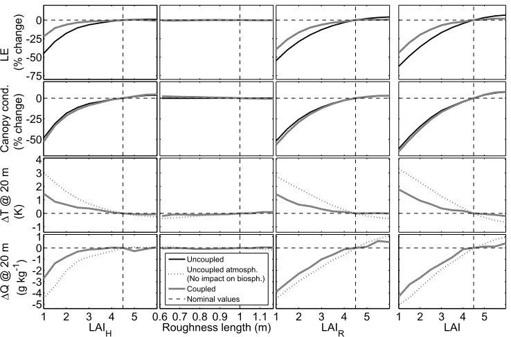
[57] With LAI reduced from 4.4 (nominal) to 1, LE was

reduced by 50%, the atmosphere was 0.7 g kg 1drier and 0.7 K warmer, and canopy conductance dropped by 65%, (Figure 8, right). Generally, the impact of decreasing LAI was greater than the impact of increasing LAI, which tended toward an asymptote for the theoretical case of infinite LAI. The response of the coupled system to LAIHand LAIRwas

similar to the system’s response to combined LAI. However, changes to the mechanical roughness of the canopy had comparatively little impact on the system. If simply summed, the impact of the three components (LAIH,LAIR

and mechanical roughness length) would have been 40 – 65% greater than the impact of just combined LAI.

5.3.2. Uncoupled Runs

[58] The uncoupled runs were generated by driving the

biosphere model with the nominal meteorology, and showed

very similar form, with generally greater impacts than the coupled runs. The exception to this rule was the response of canopy conductance, where the uncoupled runs showed greater changes.

6. Discussion

6.1. Offline Biosphere Model (SPA)

[59] The offline biosphere model corroborated well

against flux data but underpredicted LE fluxes at low LE values (Figure 2, scatterplot). This mismatch may be attrib-uted to the moss understory, which, at the SSA-OBS site, made up a surface layer 0.1 m deep. Evaporation from mosses is not stomatally controlled, but is closer mechanis-tically to simple surface evaporation [Betts et al., 1999]. SPA lacks a moss component.

[60] Soil moisture predictions were consistent with

meas-urements over the whole study period (Figure 5). Differ-ences in the modeled and measured volumetric water content at 0.25 m and 0.55 m depths were attributed to the approximate nature of the Saxton equations [Saxton et al., 1986], which were linked to soil sand, silt and clay percentages. These deviations were constant throughout the study period and, consequently, the effects of these devia-tions were negligible on the LE fluxes.

[61] Because of the increased simulated soil water

con-tent, and therefore soil thermal inertia, simulated soil temperatures might have been expected to increase more slowly than the measured soil temperatures. In fact the opposite was observed; the modeled soil temperatures at 0.25 m increased more rapidly than the data. At some points, the measured 0.25 m soil temperature was more than 5°C lower than the modeled 0.25 m layer. However, the soil energy balance can be seen to be adequate, as the off-line model was corroborated by the surface (0.05 m) and

deep (1 m) soil temperature measurements. It is likely that the 0.25 m deviations are due to heterogeneity in the soil that was not captured by the model.

[62] Compared on a half-hourly time step, the biosphere

model reproduced variability in the LE flux measurements (Figure 3). While some individual flux measurements were not explained, overall simulated fluxes were corroborated by the observations. We can be confident that, with the local meteorology, LE fluxes can be adequately simulated at the SSA-OBS site.

6.2. Fully Coupled CAB model

[63] In the CAB model, the original CAPS model cloud

routine was found to be unable to produce realistic cloud fractions, and was replaced with a fixed fraction for each day. A second reason for using a constant cloud cover faction for each day is related to the difficulties in specify-ing the whole PBL footprint’s downwellspecify-ing radiation on the basis of a single location. Cloud cover is heterogeneous and to specify a varying cloud fraction would lead to unrealistic interactions between the PBL and land surface. Instead we simplified the situation with a constant cloud fraction. As a result, the model was not expected to capture sporadic events such as cloud formation, or half hourly variations in radiation. Allowing for this, the CAB model was seen to

reproduce the correct (albeit, smoothed) downwelling short-wave radiation (Figure 3). The cause of the shift in radiation on day 250 was not identified.

[64] Because of the constant cloud fraction and the

resultant smoothing of simulated incoming shortwave radi-ation, half hourly LE fluxes were also smoothed (Figure 3). Day 250 CAB simulations show close agreement to those of the offline SPA model. However, the agreement was less good for day 167, which is consistent with the greater variability seen in the day’s observed incoming radiation.

[65] Simulated VPD agreed well with the observations

(Figure 3), however predictions deviated from the measure-ments due discrepancies between observed temperature and mixing ratio from radiosonde PBL profiles and from surface meteorology. These occurred because of the separation of the SSA-OBS tower and the radiosonde release site. Con-sequently, lower radiosonde readings represented the atyp-ical land cover at the release site. Throughout the rest of the day the model maintained a fairly consistent overestimate of VPD, but captured the correct diurnal trends. The overes-timate was relatively slight, but with some key features not being captured (early morning saturation on day 167, and the saturated above canopy air in the evening on day 250). These errors in VPD were due to relatively small simulation errors of air temperature and mixing ratio.

Figure 8. A sensitivity analysis of the CAB model, showing the response of the coupled atmosphere-biosphere system to changes in LAI, radiatively significant LAI (LAIR), roughness length, and

hydraulically significant LAI (LAIH) for day 250. Sensitivity analyses were performed using two versions

of the CAB model, the uncoupled CAB model (thin black line) and the coupled CAB model (thick gray line). Both versions of the CAB model were run for various values of LAI, LAIR, LAIH, and roughness

[66] CAB simulations of the PBL dynamics were good,

with all essential features of the PBL being captured for both days (Figures 6 and 7). Despite advection not being accounted for in the modeling scheme, mixing ratios and potential temperatures were very close to observations throughout the mixed layer, with large deviates only evident within the surface layer (lower 10% of the PBL). Visual inspection of the differences between modeled and observed PBL heights reveals that this is less than the observed variation over the region [Kiemle et al., 1997]. These results confirm that the biosphere model is effectively representing the mean response of the vegetation seen by the PBL.

[67] Advection and subsidence were not treated within

the CAB model, as is the case with most 1-D PBL models. This study relies on the assumption that the ‘‘footprint’’ of the PBL was dominated by black spruce. Fortunately the vegetation area of black spruce around the SSA is extensive, and the assumption is reasonable [Betts et al., 2001]. Application of the model in more heterogeneous landscapes would require some treatment of advection. This could be done either by footprint analysis (and a reliance on averag-ing within the PBL) [Flesch, 1996; Wilson and Swaters, 1991], or nesting within a mesoscale atmospheric model [Garratt et al., 1996]. However, both methods would represent a significant increase in the complexity of the system. In this study the CAB model was applied to explore feedbacks in a largely synthetic analysis where advection does not need to be considered.

[68] The CAB model has been simultaneously

corrobo-rated at the multiple scales of the land surface, and the boundary layer. The model explained variability in the coupled atmosphere-biosphere system, and ergo was suit-able for investigating feedbacks in the coupled system. It is important to note that the biosphere model was entirely parameterized from measurements, with the exception of plant capacitance andi, insensitive parameters which were

fitted within expected ranges. Parameters were not tuned against eddy covariance data to obtain the best fit.

6.3. CAB Model Sensitivity Analysis

6.3.1. Identifying Feedbacks Between the PBL and the Biosphere

[69] In order to identify feedbacks, we need to be able to

distinguish between the response of coupled feedback systems, and uncoupled (driven) systems. We used a simple dual sensitivity analysis focusing on changes in combined LAI (Figure 8, right).

[70] In the coupled runs, the vegetation at low combined

LAI responded to an atmosphere that was both drier and warmer than the nominal meteorology, whereas the uncoupled vegetation was driven by the nominal meteorol-ogy. The differences between the two runs were due to the effects of vegetation-atmosphere feedbacks. The analysis showed that feedbacks between the atmosphere and bio-sphere have a moderating effect, i.e., overall a negative feedback (Figure 8, right). Coupled changes due to LAI were moderated by mean values of 21% for LE, 64% for air temperature and 44% for mixing ratio, when compared to uncoupled responses. The exception was canopy conduc-tance, which the coupling increased by a mean of 9%.

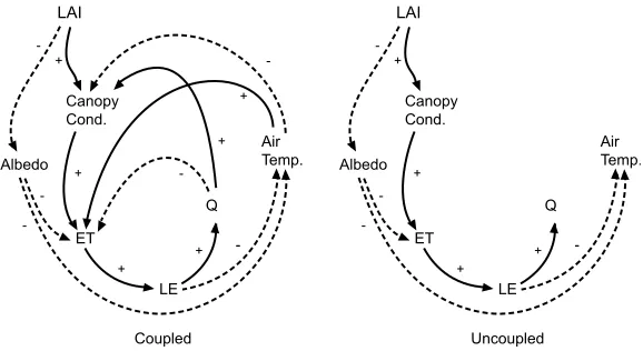
[71] The mechanisms for these effects can be thought of

as a series of positive and negative feedbacks, with some of the feedbacks absent in the uncoupled case (Figure 9). In the uncoupled case, reductions in combined LAI directly caused a drop in canopy conductance and thus evapotrans-piration (ET). These drops in ET were responsible for the warming and drying of the boundary layer in the uncoupled atmosphere (Figure 8). The direct reduction in canopy conductance resulted in a proportional reduction in the stomatal opening.

[72] For reductions in combined LAI, the coupled runs

had a lower canopy conductance than the uncoupled runs. The reduction in canopy conductance was caused by the

demand of the warmer, drier atmosphere by partially closing to limit the hydraulic tension within the plant (and the risk of cavitations in the xylem). These two basic feedback pathways allowed canopy conductance to be modified by changes in air temperature and mixing ratio (Figure 9, left). If other feedback pathways are ignored (such as the atmo-spheric impacts on ET) both of these pathways appear to allow canopy conductance to have a positive feedback on itself; that is, reduced canopy conductance reduces ET, lowering LE and resulting in a drier, warmer atmosphere and further reductions in canopy conductance.

[73] However there are competing pathways which have a

negative feedback on canopy conductance. The compara-tively warmer drier air (caused by the lowering of canopy conductance) directly increased the potential rates of ET, limiting the extent to which reduced canopy conductance warms and dries the atmosphere. This is seen in the coupled case (Figure 9, left), where the drying and warming of the boundary layer increased the atmospheric demand for water, increasing LE, but reducing canopy conductance. This feedback onto the stomata was not observed in the uncoupled case, where the coupling from the atmosphere to the vegetation was broken (Figure 9, right).

[74] Summarizing the impacts on the coupled and

uncoupled atmospheres (Figure 8, bottom two plots on the right), the coupled atmosphere-biosphere system moderated the impacts of changing LAI on the atmosphere. This moderation, acting through changes in canopy conductance, served to increase LE, under the assumption that the vegetation is not water stressed. The coupling first generates positive feedbacks, which shift the states of the atmosphere and biosphere from the uncoupled states. Negative feed-backs then stabilize the coupled system at a new steady state.

6.3.2. Relative Importance of Hydraulic, Mechanical, and Radiative Properties of the Biosphere

[75] In the sensitivity analysis, the combined LAI was

varied to investigate the impacts on the system. The analysis was then modified to separate the main contributing eco-logical factors:

[76] 1. Hydraulic impacts were as follows: LAI_Hshowed

major impacts on the coupled system (Figure 8). The uncoupled response was very similar to that of combined LAI and followed the same feedback pathways (Figure 9). Low LAIHrestricted transpiration and resulted in a warming

and drying of the atmosphere. Uncoupled runs were driven by the nominal meteorology and so were not affected by the atmospheric warming and drying. For the coupled runs, the high temperatures and drier air resulted in higher VPDs. Higher VPDs increased the LE flux, cooling and humidi-fying the resulting atmosphere (Figure 8, bottom left).

[77] 2. Mechanical roughness impacts were as follows:

Roughness length had the least impact on the coupled system (Figure 8). Impacts, although slight, were attributed to the effect of roughness length on turbulent mixing within the PBL. Greater roughness induced the surface layer to undergo more mixing with warmer, drier air from higher up in the PBL. It also caused the PBL to grow more, entraining the warm, dry air of the free atmosphere.

between the atmosphere and the stomata (Figure 8). Responses to LAIR were very similar in form and

magni-tude to the impact of LAIH, however they did not follow the

same pathways. Instead, the responses were due to increases in albedo (mainly caused by more ‘‘bright’’ soil being visible through sparser canopies), and therefore reduced absorption of radiation by the canopy. This increase in albedo should reduce fluxes of sensible heat, which should cool the atmosphere. But this did not occur as it was not the dominant process, and overall we see a replication of the warmer and drier atmosphere produced by the reduced combined LAI (Figure 8, left). In the analysis there is a similar increase in sensible heat for both reductions in combined LAI and LAIR (not shown). This is because the

dominant consequence of reduced LAIR was actually the

reduction of energy partitioned by ET into LE (Figure 9). The decreased ET was accompanied by an increased sensi-ble heat flux from the soil surface. This combination resulted in the warming and drying the coupled atmosphere. It was the physiological response of the vegetation to this warmer and drier atmosphere that then caused the reduction in stomatal conductance and therefore the moderating effect of the coupling.

[79] The coupled system response to both the LAI_H and

LAIRwas very similar in magnitude and form to that of the

combined LAI. This similarity suggests that both LAIHand

LAIR operate mainly through the same pathway (ET) and

place approximately equal limitations on rates of ET. Furthermore, the implication is that the capabilities of the black spruce for both using radiation for transpiration and for liquid phase transport were balanced for the study site. The ecosystem physiology at the SSA-OBS site seems to be balancing the two main limits on ET, on the one hand gas/ water conductance and availability, and on the other ab-sorption of incoming radiation and light use efficiency.

7. Conclusions

[80] Our biosphere model was verified by long-term data

sets and was shown to accurately simulate biosphere pro-cesses. Fluxes were correctly represented on both daily and half-hourly time scales. CAB model simulations of the PBL deviated from the observations by less than the measured variation seen over the boreal forest.

[81] Strong feedbacks occurred between the atmosphere

and biosphere, and the feedbacks tended to moderate the impacts that ecological changes had on the system. As expected, reductions in the vegetation cover tended to increase the relative partitioning into sensible heat, reducing the latent heat flux, and thus drying and heating the lower atmosphere. Calculating these effects without accounting for the effect of the vegetation’s response to the changing atmospheric conditions led to predictions that were too extreme. Furthermore, the sensitivity analysis revealed a balanced system, with both the hydrological and radiative constraints on the system being similar.

[82] This study has shown the CAB model to be a

for improvement. Several possible routes are suggested: (1) To deal with synoptic conditions, prolonged runs of the CAB model could be nudged with reanalyses of weather systems. (2) Implement a data assimilation routine to improve simulation of the PBL, through, for example, assimilation of soil moisture data or fractional cloud cover data. (3) Inclusion of the footprint analysis, or nesting the 1-D model within a mesoscale weather model to allow advection to be captured over more heterogeneous terrain and a wider range of suitable days. It should be noted that these suggestions are not mutually exclusive, and could be implemented simultaneously.

[83] Potential applications of the CAB model are diverse,

because the model runs sufficiently quickly to allow imple-mentation of numerically intensive modeling methods (e.g., inversions and data assimilation). In particular, Bayesian inversions of the model could provide a powerful means of investigating the interdependence of the model with its parameterizations and measurements. Expanding the CAB model’s capabilities would be a simple task as the model provides the framework for simulating other trace gases in the lower atmosphere.

[84] Acknowledgments. The authors would like to thank Casey Ryan, Ian Woodward, Paul Stoy, Paul Jarvis, and Shaun Quegan for their helpful comments and support during the drafting of this paper. We also thank three anonymous reviewers for useful comments. T.C.H. was funded by a NERC Studentship at the Centre for Terrestrial Carbon Dynamics.

References

Alapaty, K., and D. T. Mihailovic (2006), An intercomparison study of two land surface models using a 1-D model and FIFE measurements,Int. J. Climatol.,26, 915 – 934, doi:10.1002/joc.1266.

Anderson, D. W. (2000), General soil survey for primary sites in SSA (OA, OBS, OJP, YJP, Fen), inCollected Data of the Boreal Ecosystem-Atmosphere Study[CD-ROM], edited by J. Newcomer et al., NASA Goddard Space Flight Cent., Greenbelt, Md.

Barr, A. G., and A. K. Betts (1997), Radiosonde boundary layer budgets above a boreal forest,J. Geophys. Res.,102, 29,205 – 29,212, doi:10.1029/ 97JD01105.

Barr, A. G., and A. K. Betts (2000), Upper-air network (AFM-05) boundary layer research for BOREAS (AFM-08), inCollected Data of The Boreal Ecosystem-Atmosphere Study[CD-ROM], edited by J. Newcomer et al., NASA Goddard Space Flight Cent., Greenbelt, Md.

Barr, A., and C. Hrynkiw (2000),BOREAS AFM-5 Level-1 Upper Air Network Data,NASA Tech. Memo., NASA-TM-2000-209891, vol. 8. Barr, A. G., et al. (1997), Comparison of regional surface fluxes from

boundary-layer budgets and aircraft measurements above boreal forest,

J. Geophys. Res.,102, 29,213 – 29,218, doi:10.1029/97JD01104. Betts, A. K., and J. H. Ball (1997), Albedo over the boreal forest,

J. Geophys. Res.,102, 28,901 – 28,909, doi:10.1029/96JD03876. Betts, A. K., et al. (1999), Controls on evaporation in a boreal spruce forest,

J. Clim., 12, 1601 – 1618, doi:10.1175/1520-0442(1999)012<1601: COEIAB>2.0.CO;2.

Betts, A. K., et al. (2001), Near-surface climate in the boreal forest,

J. Geophys. Res.,106, 33,529 – 33,541, doi:10.1029/2001JD900047. Bonan, G. B., and H. H. Shugart (1989), Environmental factors and

eco-logical processes in boreal forests,Annu. Rev. Ecol. Syst.,20, 1 – 28, doi:10.1146/annurev.es.20.110189.000245.

Bounoua, L., J. Masek, and Y. M. Tourre (2006), Sensitivity of surface climate to land surface parameters: A case study using the simple biosphere model SiB2,J. Geophys. Res.,111, D22S09, doi:10.1029/2006JD007309. Chen, J. M., et al. (1997), Leaf area index of boreal forests: Theory, tech-niques, and measurements, J. Geophys. Res., 102, 29,429 – 29,443, doi:10.1029/97JD01107.

Cionco, R. M. (1985), Modeling windfields and surface layer wind profiles over complex terrain and within vegetative canopies, inThe Forest-Atmosphere Interaction, edited by B. A. Hutchison and B. B. Hicks, pp. 501 – 520, D. Reidel, Dordrecht, Netherlands.

Cox, P. M., et al. (2000), Acceleration of global warming due to carbon-cycle feedbacks in a coupled climate model,Nature,408, 184 – 187, doi:10.1038/35041539.

Crossley, J. F., et al. (2000), Uncertainties linked to land-surface processes in climate change simulations,Clim. Dyn.,16, 949 – 961, doi:10.1007/ s003820000092.

Cuenca, R. H. (2000), Coupled atmosphere-forest canopy-soil profile monitoring and simulation, inCollected Data of The Boreal Ecosystem-Atmosphere Study[CD-ROM], edited by J. Newcomer et al., NASA God-dard Space Flight Cent., Greenbelt, Md.

Cuenca, R. H., et al. (1996), Impact of soil water property parameterization on atmospheric boundary layer simulation,J. Geophys. Res.,101, 7269 – 7277, doi:10.1029/95JD02413.

Cuenca, R. H., et al. (1997), Soil water balance in a boreal forest,

J. Geophys. Res.,102, 29,355 – 29,365, doi:10.1029/97JD02312. Davis, K. J., et al. (1997), Role of entrainment in surface-atmosphere

inter-actions over the boreal forest,J. Geophys. Res.,102, 29,219 – 29,230, doi:10.1029/97JD02236.

Denning, A. S., et al. (2003), Simulated variations in atmospheric CO2over a Wisconsin forest using a coupled ecosystem-atmosphere model,Global Change Biol.,9, 1241 – 1250, doi:10.1046/j.1365-2486.2003.00613.x. Desborough, C. E., et al. (2001), Surface energy balance complexity in

GCM land surface models. Part II: Coupled simulations, Clim. Dyn.,

17, 615 – 626, doi:10.1007/s003820000131.

Ek, M. B., and A. A. M. Holtslag (2004), Influence of soil moisture on boundary layer cloud development, J. Hydrometeorol., 5, 86 – 99, doi:10.1175/1525-7541(2004)005<0086:IOSMOB>2.0.CO;2.

Engel, V. C., et al. (2002), Forest canopy hydraulic properties and catch-ment water balance: Observations and modeling, Ecol. Modell.,154, 263 – 288, doi:10.1016/S0304-3800(02)00068-6.

Environment Canada (2004), Monthly data report for 1994, Gatineau, Que., Canada. (Available at http://www.climate.weatheroffice.ec.gc.ca/ climateData/canada_e.html)

Essery, R. L. H., et al. (2003), Explicit representation of subgrid hetero-geneity in a GCM land surface scheme,J. Hydrometeorol.,4, 530 – 543, doi:10.1175/1525-7541(2003)004<0530:EROSHI>2.0.CO;2.

Ewers, B. E., et al. (2005), Effects of stand age and tree species on canopy transpiration and average stomatal conductance of boreal forests,Plant Cell Environ.,28, 660 – 678, doi:10.1111/j.1365-3040.2005.01312.x. Farquhar, G. D., and S. Craemmerer (1982), Modelling of photosynthetic

response to the environment, inPhysiological Plant Ecology II, edited by O. L. Lange et al., pp. 549 – 587, Springer, Berlin.

Fisher, R. A., et al. (2006), Evidence from Amazonian forests is consistent with isohydric control of leaf water potential,Plant Cell Environ.,29, 151 – 165, doi:10.1111/j.1365-3040.2005.01407.x.

Flesch, T. K. (1996), The footprint for flux measurements, from backward Lagrangian stochastic models,Boundary Layer Meteorol.,78, 399 – 404, doi:10.1007/BF00120943.

Garratt, J. R., et al. (1996), The atmospheric boundary layer—Advances in knowledge and application, Boundary Layer Meteorol., 78, 9 – 37, doi:10.1007/BF00122485.

Goulden, M. L., et al. (1996), Measurements of carbon sequestration by long-term eddy covariance: Methods and a critical evaluation of accuracy, Glo-bal Change Biol.,2, 169 – 182, doi:10.1111/j.1365-2486.1996.tb00070.x. Guichard, F., et al. (2004), Modelling the diurnal cycle of deep precipitating convection over land with cloud-resolving models and single-column models,Q. J. R. Meteorol. Soc.,130, 3139 – 3172, doi:10.1256/qj.03.145. Henderson-Sellers, A., et al. (1993), The Project for Intercomparison of Land-Surface Parameterization Schemes,Bull. Am. Meteorol. Soc.,74, 1335 – 1349, doi:10.1175/1520-0477(1993)074<1335:TPFIOL>2.0. CO;2.

Henderson-Sellers, A., et al. (1995), The Project for Intercomparison of Land-Surface Parameterization Schemes (PILPS): Phases 2 and 3,Bull. Am. Meteorol. Soc., 76, 489 – 503, doi:10.1175/1520-0477(1995)076< 0489:TPFIOL>2.0.CO;2.

Hollinger, D. Y., and A. D. Richardson (2005), Uncertainty in eddy covar-iance measurements and its application to physiological models, Tree Physiol.,25, 873 – 885.

Holtslag, A. A. M., and M. Ek (1996), Simulation of surface fluxes and boundary layer development over the pine forest in HAPEX-MOBILHY,

J. Appl. Meteorol.,35, 202 – 213, doi:10.1175/1520-0450(1996)035< 0202:SOSFAB>2.0.CO;2.

Holtslag, A. A. M., and A. P. Vanulden (1983), A simple scheme for day-time estimates of the surface fluxes from routine weather data,J. Clim. Appl. Meteorol.,22, 517 – 529, doi:10.1175/1520-0450(1983)022<0517: ASSFDE>2.0.CO;2.

Holtslag, A. A. M., et al. (1990), A high-resolution air-mass transformation model for short-range weather forecasting, Mon. Weather Rev., 118, 1561 – 1575, doi:10.1175/1520-0493(1990)118<1561:AHRAMT>2.0. CO;2.

Jarvis, P. G., and J. B. Moncrieff (2000), The CO2exchanges of boreal black spruce forest, inCollected Data of The Boreal Ecosystem-Atmosphere Study[CD-ROM], edited by J. Newcomer et al., NASA Goddard Space Flight Cent., Greenbelt, Md.

Jarvis, P. G., et al. (1997), Seasonal variation of carbon dioxide, water vapor, and energy exchanges of a boreal black spruce forest,J. Geophys. Res.,102, 28,953 – 28,966, doi:10.1029/97JD01176.

Jones, H. G. (1992),Plants and Microclimate: A Quantitative Approach to Environmental Plant Physiology, 2nd ed., 428 pp., Cambridge Univ. Press, Cambridge, U. K.

Kiemle, C., et al. (1997), Estimation of boundary layer humidity fluxes and statistics from airborne differential absorption lidar (DIAL),J. Geophys. Res.,102, 29,189 – 29,203, doi:10.1029/97JD01112.

Koster, R. D., et al. (2006), GLACE: The Global Land-Atmosphere Cou-pling Experiment. Part I: Overview,J. Hydrometeorol.,7, 590 – 610, doi:10.1175/JHM510.1.

Lee, Y.-H., and L. Mahrt (2004), Comparison of heat and moisture fluxes from a modified soil-plant-atmosphere model with observations from BOREAS,J. Geophys. Res.,109, D08103, doi:10.1029/2003JD003949. Mahrt, L., and H. Pan (1984), A 2-layer model of soil hydrology,Boundary

Layer Meteorol.,29, 1 – 20, doi:10.1007/BF00119116.

Miller, J. R., et al. (1997), Seasonal change in understory reflectance of boreal forests and influence on canopy vegetation indices,J. Geophys. Res.,102, 29,475 – 29,482, doi:10.1029/97JD02558.

Monteith, J. L. (1965), Evaporation and environment, in Symposia of the Society for Experimental Biology, vol. 19, edited by G. E. Fogg, pp. 205 – 234, Cambridge Univ. Press, Cambridge, U. K.

Murthy, B. S., et al. (2004), Interactions of the land-surface with the atmo-spheric boundary layer: Case studies from LASPEX,Curr. Sci., 86, 1128 – 1134.

Nemati, M. R., et al. (2002), Determining air entry value in peat substrates,

Soil Sci. Soc. Am. J.,66, 367 – 373.

Newcomer, J., et al. (Ed.) (2000),Collected Data of the Boreal Ecosystem-Atmosphere Study, NASA Goddard Space Flight Cent., Greenbelt, Md. Penman, H. L. (1948), Natural evaporation from open water, bare soil and

grass,Proc. R. Soc. London, Ser. A,193, 120 – 145.

Rayment, M. B., et al. (2002), Photosynthesis and respiration of black spruce at three organizational scales: Shoot, branch and canopy,Tree Physiol.,22, 219 – 229.

Ryan, M. G. (2000), Introduction to BOREAS special issue,Tree Physiol.,

20, 709 – 711.

Saxton, K. E., et al. (1986), Estimating generalized soil-water characteris-tics from texture,Soil Sci. Soc. Am. J.,50, 1031 – 1036.

Schwarz, P. A., B. E. Law, M. Williams, J. Irvine, M. Kurpius, and D. Moore (2004), Climatic versus biotic constraints on carbon and water fluxes in seasonally drought-affected ponderosa pine ecosystems,Global Biogeo-chem. Cycles,18, GB4007, doi:10.1029/2004GB002234.

doi:10.1029/97JD03300.

Seneviratne, S. I., et al. (2006), Land-atmosphere coupling and climate change in Europe,Nature,443, 205 – 209, doi:10.1038/nature05095. Steele, S. J., et al. (1997), Root mass, net primary production and turnover

in aspen, jack pine and black spruce forests in Saskatchewan and Man-itoba, Canada,Tree Physiol.,17, 577 – 587.

Stull, R. B. (1988),An Introduction to Boundary Layer Meteorology, Kluwer Acad., Dordrecht, Netherlands.

Troen, I., and L. Mahrt (1986), A simple model of the atmospheric bound-ary layer: Sensitivity to surface evaporation,Boundary Layer Meteorol.,

37, 129 – 148, doi:10.1007/BF00122760.

van Wijk, M. T., et al. (2003), Interannual variability of plant phenology in tussock tundra: Modelling interactions of plant productivity, plant phe-nology, snowmelt and soil thaw,Global Change Biol.,9, 743 – 758, doi:10.1046/j.1365-2486.2003.00625.x.

van Wijk, W. R. (1963),Physics of Plant Environment, 382 pp., North-Holland, Amsterdam.

Williams, M., et al. (1996), Modelling the soil-plant-atmosphere continuum in a Quercus-Acer stand at Harvard forest: The regulation of stomatal conductance by light, nitrogen and soil/plant hydraulic properties,Plant Cell Environ., 19, 911 – 927, doi:10.1111/j.1365-3040.1996.tb00456.x 2000.

Williams, M., et al. (1997), Predicting gross primary productivity in terres-trial ecosystems, Ecol. Appl., 7, 882 – 894, doi:10.1890/1051-0761(1997)007[0882:PGPPIT]2.0.CO;2.

Williams, M., et al. (2000), The controls on net ecosystem productivity along an Arctic transect: A model comparison with flux measurements,

Global Change Biol., 6, 116 – 126, doi:10.1046/j.1365-2486.2000. 06016.x.

Williams, M., et al. (2001), Use of a simulation model and ecosystem flux data to examine carbon-water interactions in ponderosa pine,Tree Phy-siol.,21, 287 – 298.

Wilson, J. D., and G. E. Swaters (1991), The source area influencing a measurement in the planetary boundary layer: The footprint and the dis-tribution of contact distance,Boundary Layer Meteorol., 55, 25 – 46, doi:10.1007/BF00119325.

Wood, E. F., et al. (1998), The Project for Intercomparison of Land-surface Parameterization Schemes (PILPS) phase 2 (c) Red-Arkansas River basin experiment: 1. Experiment description and summary intercomparisons,

Global Planet. Change, 19, 115 – 135, doi:10.1016/S0921-8181(98) 00044-7.