Stability Assessment of High-Bandwidth DC Voltage Controllers in
Single-Phase Active-Front-Ends: LTI vs LTP Models
Valerio Salis,
Member, IEEE,
Alessandro Costabeber,
Member, IEEE,
Stephen M. Cox,
Andrea Formentini,
Member, IEEE
and Pericle Zanchetta,
Senior Member, IEEE,
February 26, 2018
Abstract—In recent years, a considerable effort has been made to minimise the size of DC-link capacitors in single-phase active-front-ends (SP-AFE), to reduce cost and to increase power density. As a result of the lower energy storage, a high-bandwidth outer DC voltage control loop is required to respond to fast load changes. Linearised modelling is usually performed according to the power-balance method and the control is designed using LTI techniques. This is done assuming negligible voltage ripple at twice the grid frequency, and the model is considered valid up to the grid frequency. However, its precise validity limits are usually unknown and the control design becomes empirical when approaching these boundaries. To overcome this drawback, Linear Time Periodic (LTP) theory can be exploited, defining the range of validity of the LTI model and providing precise stability boundaries for the DC-link voltage loop. The main result is that LTP models more accurately describe the system behaviour and provide superior results compared to the LTI ones. Theoretical analysis, simulations and extensive experimental tests on a 10 kW converter are presented to validate the claims.
Index Terms—Linear Time Periodic Systems, Harmonic State Space Model, Stability Analysis, Power Converters, Active-Front-Ends
I. INTRODUCTION
T
HE use of electrolytic capacitors as energy buffers is the most common approach to stabilize the DC-link voltage in single-phase converters. A large capacitor has a dual well-known positive effect: it reduces the steady-state voltage ripple and minimises voltage overshoots and undershoots caused by load changes. The large amount of stored energy can compensate the variations in the power absorbed by the load, guaranteeing small voltage over-undershoots even with a slow voltage control loop. However, a large electrolytic capacitor has also major disadvantages: low power density and reduced reliability due to the short lifetime expectancy caused by temperature degradation. Furthermore, regular maintenance is required to prevent ageing effects. Thus, its replacement withV. Salis, A. Costabeber, P. Zanchetta and A. Formentini are with the De-partment of Electrical and Electronic Engineering, University of Nottingham, Nottingham NG7 2RD, U.K. (e-mail: [email protected]; [email protected]; [email protected]; [email protected]).
S. M. Cox is with the School of Mathematical Sciences, University of Nottingham, Nottingham NG7 2RD, U.K. (e-mail: [email protected]).
the more reliable film capacitor, despite the smaller capaci-tance, has been the object of several research contributions over the years [1], [2].
The use of smaller DC-link capacitance overcomes the lim-itations of electrolytic capacitors, but also their advantages are lost. In fact, a smaller capacitor leads to larger voltage ripple and, due to the smaller amount of energy that it can store, it cannot counteract voltage over-undershoots caused by load changes. These two problems are usually addressed separately: the higher ripple is generally handled by implementing more sophisticated voltage controllers, whereas the over-undershoot is generally dealt with using faster voltage controllers [3]–[9]. Typical systems where DC-link capacitor reduction is highly beneficial are the SP-AFEs, representing the simplest and most popular grid-connected converter where a non-linear control loop is required, i.e. the outer DC voltage loop. The design of the DC voltage control loop is typically based on the assumption that the loop will have a bandwidth set to a fraction of the grid frequency, so that sufficient decoupling of the second harmonic DC voltage ripple from the AC current can be achieved, thus reducing distortion of the AC current reference [10]. As a consequence, an average model based on power balance, valid for the low frequencies of interest, can be used to overcome the fundamental issue of having a non-linear control loop involving AC quantities. On the other hand, little attention has been given in the literature to the analytical modelling of the impact of a given design bandwidth on the actual eigenvalues of the closed-loop system. This is because when a large DC-link capacitor is used, a fast voltage control loop is not required. However, the reduction of the capacitor size demands a high-bandwidth voltage loop, in order to keep voltage over-undershoots within the system specifications. In this scenario, the application of standard techniques might lead to a poorly damped or unstable control solution because the design target falls beyond the remit of the power-based model [11].
for low bandwidth of the voltage controller the dominant closed-loop poles of the system calculated with both LTI and LTP approaches are consistent. The additional contribution of the paper is to show how for higher bandwidths the actual eigenvalues can be calculated correctly only with the LTP model, and the LTI model is no longer valid. This leads to a set of guidelines for the design of fast DC-link voltage controllers for the system under study, highlighting the limits of LTI design methods and providing a prediction of the actual system eigenvalues when the LTI-based design is performed close to or beyond its validity boundaries. This has been done on the assumption that the designer typically prefers to use established control design techniques rather than exploring completely different methods based on other theories. Additional comparisons between LTI and LTP models are reported in [12].
Note that the proposed analysis is developed here for a simple single-phase active-front-end topology where power density and/or reliability are increased simply by replacing the DC-link capacitor with a smaller one. The rationale for this choice is that those systems are the most common ones, and their relatively low complexity enables an easier introduction of LTP models. However, similar considerations hold for the family of topologies where the DC capacitor is reduced using dedicated ripple ports, as reported by several recent contributions such as [13]–[16], or for the topologies where the input current is distorted [17].
The basic principles of the LTP analysis are given in [18], [19]. A generic AC system like the SP-AFE under study can be equivalently represented by an average model that is Non-Linear and Time Periodic (NLTP), where in steady-state all the state-space variables are time periodic, with period given by the fundamental AC frequency. When linearisation of the NLTP model is performed around its steady-state trajectory, an LTP system is obtained, which is the key to the design and stability analysis method exploited in this paper. From the LTP model, the Harmonic State Space (HSS) model is derived. The purpose of such a model is generally twofold. First it permits the replacement of a non-linear circuit with its HSS model. Such a model requires less computation time in the simulation process, yet harmonic interaction and couplings are still properly taken into account. Examples of HSS model derivations are given in [20] for a controlled TCR and in [21] for a grid-connected converter. A general approach to derive HSS models is proposed in [22] for linear and switching subsystems.
Second, once the HSS model has been derived, stability analysis can be performed: in [23] stability analysis is carried out on a locomotive single-phase grid-connected converter; in [24] and [25] a single-phase grid-connected converter with DC-link capacitor is considered, while in [26] the analysis of a grid-connected converter with PLL is reported.
Note that a comprehensive inclusion of all the high fre-quency dynamics of the converter into the model is beyond the scope of this work, which is instead focused on the impact of non-linearity of the DC voltage control loop on stability. This normally affects stability in the low-frequency range, i.e. below the bandwidth of the inner current controller.
There are also other approaches presented in literature, like the Dynamic-Phasor method [27], exploited for the stability analysis of a system comprising a source and a load single-phase converter, or [28], where a three-single-phase Voltage Source Inverter is analysed both in dq andαβ frames. However, in both cases there is no outer DC-link control, and currents and voltages in these systems have only a dominant component at the grid frequency, which allows the application of these methods. In the system analysed in this paper, not only the dominant component, but also the DC and second harmonic are naturally taken into account by the LTP analysis. This is arguably one of the advantages of exploiting the LTP approach, since one can consider any number of harmonics in an intuitive way. Nevertheless, in the literature some efforts to enhance the above methods in order to overcome the dominant-component limitation can be found [29], and a detailed comparison with the LTP approach is an interesting and new research direction. The main contributions of the paper can be summarised as follows:
(1) the limit of validity of LTI model in SP-AFE systems has been, for the first time, rigorously determined and a precise description of the system above this limit has been presented;
(2) the use of LTP model (refer to Fig. 5-6-7) for enhanced analysis, and also the possibility to improve the system performance above the limit of validity of the LTI model (for example, using a different pole placement and check-ing the actual location of the closed-loop eigenvalues) has been discussed;
(3) a guidance through all the necessary steps and practical considerations required to extend this analysis method to any application based on power converters has been presented.
The paper is organized as follows: Section II provides a description of the active-front-end system and the derivation of the average model; in Section III a brief review of the main features of LTP theory is reported; in Section IV the steady-state solutions are evaluated and these are used in Section V to calculate the LTP system, on which the eigenvalue analysis is applied; in Section VI, analytical, simulation and experimental results are presented for a 10 kW prototype, showing how the LTP model can predict the closed loop eigenvalues of the system where the LTI modelling and design approach lose validity.
II. SINGLE-PHASEACTIVE-FRONT-END- NONLINEAR AVERAGEMODEL
for frequencies below that of the grid. However, a precise validity limit is usually unknown. When a small DC-link capacitor is used and fast DC-link voltage control is required, the design bandwidth of the controller must be increased, thus going beyond the limit of validity of (2) and leading to an uncertain result. Thus, the LTP theory will be applied in order to provide a precise answer to the aforementioned problems. The range of validity of the LTI model (2) will be evaluated. Moreover, when the design bandwidth of the voltage controller is increased beyond the validity boundaries of the LTI approach, a correct stability assessment will be possible only by exploiting the LTP approach. In the system under analysis, the current PI control is designed based on the linearised open-loop transfer function:
GI(s) =
1
(sLg+Rg), (1)
where Lg is the grid inductance and Rg is its parasitic
resistance, in order to guarantee that the LTI closed-loop transfer function HI(s) = P II(s)GI(s)/(1 +P II(s)GI(s))
has a bandwidth of 1 kHz and a 70o phase margin. This
control is then kept constant during all the simulations and the experiments. In contrast, the voltage PI control design is based on the linearised open-loop transfer function that can be easily derived from the power balance approach [10]:
GV(s) = V
2
gRdc
2Vref(2 +sRdcCdc), (2)
withVgbeing the peak grid voltage,Vref the reference for the DC-link voltage, Rdc the resistive load andCdc the DC-link capacitor. A set of closed-loop design bandwidths is chosen, reported in Table II, and for each of them the voltage PI gains are calculated according to (2), considering a constant design phase margin of 70o. The reference to ‘design bandwidth’
rather than simply ‘bandwidth’ is due to the fact that the designed one and the actual one will match only when the LTI model is within its validity boundaries. By exploiting the LTP theory, the following analyses can be performed:
• The calculation of the maximum design bandwidth,Bw, for which the actual eigenvalues of the voltage loop are consistent with those calculated using the LTI model, thus providing the range of validity of (2).
• The actual stability boundary of the system, i.e. the max-imum value of design bandwidth Bwmax, not necessarily
within the range of validity of the LTI approach, below which the actual system is stable and above which it is unstable.
For simplicity, the control is initially designed in the continuous-time domain, and all the LTP analysis is applied to the continuous system. For the experimental validation, the controllers are discretized with sampling timeTsfor the digital implementation. The effect of the computational delay, Ts, as well as the delay introduced by the zero-order hold (ZOH) of the PWM, approximated by 0.5Ts, are taken into account in order to provide an accurate continuous model of the system for LTP analysis. It will be shown that the system instability arises at relatively low frequencies, thus the discretization method does not substantially affect the subsequent analysis.
+
PWM
1
s
1
s s2
2 s dc R dc C g
R Lg
1
s s2
ZOH s sT e ref V 1 + -g v g v + PII + -* * g v
PIV NOTCH
-+ Vref
dc v dc
v
g i ref g i _Fig. 1.Schematic and control of the single-phase active-front-end.
These delays are included in the analysis using their equivalent continuous-time transfer functions [30]:
H(s) =e−sTs
1−e−sTs
/(sTs). (3)
The complex exponential is replaced with a first-order Pad´e approximation of the form
e−sTs= (n
1s+n0)/(d1s+d0). (4)
Substituting (4) in (3) gives the transfer function
H(s) = (γ1s+γ0)/(s2+σ1s+σ0), (5)
which relates the output of the current controller to the duty cycle. The notch filter transfer function is:
N(s) =kn+ (p1s+p0)/(s2+q1s+q0), (6)
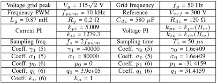
which is tuned to attenuate the DC-link voltage ripple at2ωg. The system parameters are summarised in Table I.
TABLE I.System parameters
Voltage grid peak Vg= 115 √
2V Grid frequency fg= 50 Hz
Frequency PWM fpwm= 10 kHz Reference Vref = 300 V
Lg= 0.87 mH Rg= 0.2Ω Cdc= 580µF Rdc= 120Ω
Current PI kpi= 5.009 Voltage PI kpv=kpv(Bw) kii= 1279.3 kiv=kiv(Bw)
Sampling freq. fs= 2fpwm Sampling time Ts= 50µs
Coeff.γ1(5) γ1= -40000 Coeff.γ0(5) γ0= 1.6e+09
Coeff.σ1(5) σ1= 80000 Coeff.σ0(5) σ0= 1.6e+09
Coeff.p0(6) p0= 0 Coeff.p1(6) p1= -31.4159
Coeff.q0(6) q0= 3.9e+05 Coeff.q1(6) q1= 31.4159
Coeff.kn(6) kn= 1
The switching system is replaced by its continuous-time average equivalent model and the stability analysis is per-formed on the latter. As shown later, the instability arises at frequencies far below that of the switching, so for the purposes of this work using the average model provides accurate results. The average model of the system is described by the state-space model (7) (where the time dependency of the variables is omitted for brevity), which is an eighth-order NLTP system, with all the states being Tg-periodic and the non-linearities being given by the productsxixj. The statesx1,x2 describe
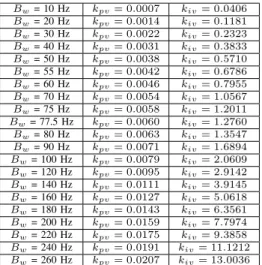
TABLE II. Voltage PI controller parameters for each DC voltage design bandwidth
Bw= 10 Hz kpv= 0.0007 kiv= 0.0406
Bw= 20 Hz kpv= 0.0014 kiv= 0.1181
Bw= 30 Hz kpv= 0.0022 kiv= 0.2323
Bw= 40 Hz kpv= 0.0031 kiv= 0.3833
Bw= 50 Hz kpv= 0.0038 kiv= 0.5710
Bw= 55 Hz kpv= 0.0042 kiv= 0.6786
Bw= 60 Hz kpv= 0.0046 kiv= 0.7955
Bw= 70 Hz kpv= 0.0054 kiv= 1.0567
Bw= 75 Hz kpv= 0.0058 kiv= 1.2011
Bw= 77.5 Hz kpv= 0.0060 kiv= 1.2760
Bw= 80 Hz kpv= 0.0063 kiv= 1.3547
Bw= 90 Hz kpv= 0.0071 kiv= 1.6894
Bw= 100 Hz kpv= 0.0079 kiv= 2.0609
Bw= 120 Hz kpv= 0.0095 kiv= 2.9142
Bw= 140 Hz kpv= 0.0111 kiv= 3.9145
Bw= 160 Hz kpv= 0.0127 kiv= 5.0618
Bw= 180 Hz kpv= 0.0143 kiv= 6.3561
Bw= 200 Hz kpv= 0.0159 kiv= 7.7974
Bw= 220 Hz kpv= 0.0175 kiv= 9.3858
Bw= 240 Hz kpv= 0.0191 kiv= 11.1212
Bw= 260 Hz kpv= 0.0207 kiv= 13.0036
with the voltage PI control; x4 is associated with the current
PI control; x5 andx6 represent the internal dynamics of the
computational delay, ZOH and PWM; x7 represents the grid
current, ig;x8 the DC-link voltage, vdc, and the grid voltage
(input) is vg=Vgsin(ωgt):
d=Vref−1vg−kiix4−kpikivvgx3−kpikpvp0vgx1,
−kpikpvp1vgx2−kpikpvknvg(Vref −x8) +kpix7
˙
x1=x2 , x˙2=−q0x1−q1x2+Vref −x8,
˙
x3=p0x1+p1x2+kn(Vref−x8),
˙
x4=kivvgx3+kpvp0vgx1+kpvp1vgx2+kpvknvg(Vref −x8)
−x7 , x˙5=x6 , x˙6=−σ0x5−σ1x6+d,
˙
x7=L−g1[vg−Rgx7−γ0x5x8−γ1x6x8],
˙
x8=Cdc−1γ0x5x7+γ1x6x7−R−dc1x8. (7)
III. BASICTHEORY FOR THESTABILITYANALYSIS OF LTP SYSTEMS
A comprehensive review of the basics of LTP theory is reported in [31], [32], and only a brief summary is given here, mainly to clarify the notation. Once the steady-state operating conditions have been found from the NLTP system (7), the stability may be determined by linearising the NLTP system around the steady-state periodic operating trajectory [33], [34], which gives an LTP system on which the stabil-ity analysis is performed. Following this procedure, given a steady-state input u¯, a steady-state solution of the system (7),
¯
x, is obtained either analytically, as described in section V of this paper, or numerically (using fsolve in Matlab, for example), depending on the complexity of the system. Then linearisation is applied, which requires the addition of a small-signal perturbation to the steady-state input, output and state-space variables: f(t) = ¯f(t) + ˜f(t) ,with f =u, x, y. This leads to the linearised model, which is an LTP system of the form
˙˜
x(t) =A(t)˜x(t) +B(t)˜u(t),
˜
y(t) =C(t)˜x(t) +D(t)˜u(t). (8)
All the matricesA(t),B(t),C(t)andD(t)areT-periodic, whereT is the period of the steady-state solution. Exploiting the Exponentially Modulated Periodic (EMP) signal [18], [19] as input to the LTP system, which is defined as
u(t) =ejΩt
+∞
X
n=−∞
unejnωTt, (9)
where ωT = 2π/T, it follows that also the state-space
variables and the output are EMP signals, thus making it possible to define the transfer function operator. To this end, the Toeplitz transformation is introduced and will be used throughout the rest of this work. To define the Toeplitz transformation, consider a T-periodic matrix F(t) (i.e. one whose coefficients are all T-periodic functions). Then the Toeplitz transformation is given by
T[F(t)] =F= .. . ... ... · · · F0 F−1 F−2 · · ·
· · · F1 F0 F−1 · · ·
· · · F2 F1 F0 · · ·
.. . ... ... , (10)
which is a doubly infinite block-Toeplitz matrix with matrices
Fi that are the Fourier matrix coefficients of the T-periodic matrixF(t). This transformation is applied to all the matrices and vectors in (8). By suitable manipulations [31], the Har-monic State-Space Model (HSSM) of the LTP system can be derived as
sX = (A − N)X+BU,
Y=CX +DU, (11)
with N = diag(. . . , N−n, . . . , N−1, N0, N1, . . . , Nn, . . .),
Nn being a diagonal square matrix of the same dimension as An with diagonal coefficients equal to jnωT. The system (11) is time-invariant. Hence calculation may now proceed as in the LTI case; in particular, the Harmonic Transfer Function (HTF) of the LTP system is defined as follows:
Y= ˆG(s)U, Gˆ(s) =C[sI −(A − N)]−1B+D. (12) Stability analysis can now be addressed through the evalua-tion of the eigenvalue loci of the matrixA − N. In fact, if all the eigenvalues haveRe[λi]≤0, where those withRe[λi] = 0
have algebraic multiplicity equal to1, then the system is stable, otherwise the system is unstable.
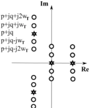
A practical implementation of the LTP theory requires a truncation order N, based on the number of harmonics taken into account. For example, N = 2 means including DC-component, first and second harmonics, with all the others set to zero. Increasing the truncation orderN leads to a more precise evaluation of the system stability, but the dimension of the Toeplitz form also increases. Also the dimension of the matrixA − N increases withN, with a higher number of associated eigenvalues. To clarify this, an LTP system of order
as significant eigenvalues, are necessary to assess the stability of the system. The other 2N ×m eigenvalues are copies of the significant ones, but shifted by jnωT,n=±1, . . . ,±N.
Fig. 2 shows an example of a typical plot of eigenvalue loci for a LTP system of orderm= 4and truncation orderN = 2. The stars depict the significant eigenvalues, while with circles represent their translated copies.
Fig. 2.Generic eigenvalue loci of an LTP system: stars - significant eigenvalues; circles - translated copies
One final aspect is the choice of the truncation order. The theoretical analysis is based on infinite harmonic series and a sufficiently high value for the truncation order, N∗, must be chosen so that the location of the significant eigenvalues is robust. Above N = N∗, the position of the significant eigenvalues should not change, but below N = N∗, the eigenvalues move from their correct position and an incorrect plot of their loci is obtained. This implies that, to obtain accurate results, the truncation order must be chosen with
N ≥ N∗. The quantification of N∗ is discussed in section VI.
IV. STEADY-STATESOLUTION
In order to perform a stability analysis based on the LTP model, first the steady-state trajectories of the NLTP system (7) must be calculated. Only the calculation of the steady-state variables involved in the LTP model (18) is considered, which are x¯5,x¯6,x¯7 andx¯8. From the power-balance approach, the
steady-state voltage on the DC-link capacitor is given by
¯
vdc= ¯x8=Vref− Vref
2ωgCdcRdcsin(2ωgt) = ¯x80−x¯82, (13)
i.e. it is the sum of a DC component,x¯80, and a second-order
harmonic, x¯82, which is the ripple at 2fg. The amplitude of
this ripple depends on the value of the DC-link capacitor, and clearly does not depend on the actual gains of the controller. The inductor current is given by
¯ig= ¯x7= 2V
2
ref
VgRdcsin(ωgt). (14)
Finally, the internal dynamics of the unit computational delay, ZOH and PWM blocks are represented by the state-space model
˙¯
x5
˙¯
x6
=
0 1
−σ0 −σ1
¯
x5
¯
x6
+
0 1
¯
d. (15)
Defining Aσ = [0 1;−σ0 −σ1], Bσ = [0; 1], the
trans-fer functions relating the input to each of the state-space
variables are H5(s) = [1 0] [sI−Aσ] −1
Bσ and H6(s) =
[0 1] [sI−Aσ] −1
Bσ, with d¯= vg/Vref being the
approxi-mated input. Thus the last two steady-state solutions are given by
¯
x5=|H5(jωg)|VgVref−1sin(ωgt+ H5(jωg)), (16)
¯
x6=|H6(jωg)|VgVref−1sin(ωgt+ H6(jωg)). (17)
V. LINEARISEDMODEL(LTP)
Based on the steady-state solutions from the previous sec-tion, the LTP model is derived following the linearisation illustrated in section III, yielding a system of the form
˙˜
x(t) = A(t)˜x(t), with A(t) being a Tg-periodic matrix, as shown in (18). When the Fourier series expansion is applied toA(t), the only Fourier coefficients different from zero are
A0, A±1 and A±2, since the steady-state solution contains
harmonic coefficients only up to the second harmonic. The Toeplitz transformation is applied to the LTP system (18), and from a study of the eigenvalue loci ofA − N, as in (11) and (12), the actual eigenvalues of the system are determined. The full derivation is not reported for the sake of brevity but all the Toeplitz forms and the Harmonic State Space model can be directly derived from the LTP state-space system below:
˙˜
x1= ˜x2 , x˙˜2=−q0x˜1−q1x˜2−x˜8,
˙˜
x3=p0x˜1+p1x˜2−knx˜8,
˙˜
x4=kivvgx˜3+kpvp0vgx˜1+kpvp1vgx˜2−kpvknvgx˜8−x˜7,
˙˜
x5= ˜x6 , x˙˜6=−σ0x˜5−σ1x˜6−kiiVref−1˜x4
−kpikivvgVref−1˜x3−kpikpvp0vgVref−1x˜1
−kpikpvp1vgVref−1x˜2+kpikpvknvgVref−1x˜8+kpiVref−1x˜7,
˙˜
x7=L−g1
−Rgx˜7−γ0x¯5x˜8−γ0x¯8(t)˜x5−γ1x¯6x˜8
−γ1x¯8x˜6,
˙˜
x8=Cdc−1
γ0x¯5x˜7+γ0¯x7x˜5+γ1x¯6x˜7+γ1x¯7x˜6−x˜8R−dc1
.
(18)
In the next section, the LTP model (18), in HSS form, will be exploited to evaluate the validity of the basic LTI model for DC voltage control design. It will be shown that the LTP model provides high accuracy in the identification of the stability boundaries of the system, and can therefore be used to identify the limits of validity of the voltage control design based on the LTI model.
VI. ANALYTICAL, SIMULATION ANDEXPERIMENTAL RESULTS
A. Eigenvalue Analysis
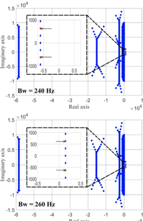
1) Validity boundaries of the LTI model: Based on (18) and on Tables I and II, the theoretical evaluation of the actual eigenvalues of the SP-AFE is performed based on the LTP eigenvalue loci-plot of the matrix A − N. The first result concerns the maximum value of the LTI‘design bandwidth’
for which the system is stable, which is found to beBw= 240
as shown in Fig. 3 (bottom - indicated by arrows), leading to instability.
Six vertical lines of eigenvalues form the LTP eigenvalue loci-plot. An initial truncation order N = 30 has been chosen, which guarantees an accurate eigenvalue plot. It can be observed that not all the eigenvalues lie on these vertical lines. The translated copies that are furthest from the significant eigenvalues suffer from the effects of the truncation, thus they must not be considered in the stability analysis as they do not have physical meaning. We will refer to these as spurious eigenvalues.
Fig. 3. LTP eigenvalue loci plot with N = 30: (top), stable system withBw= 240Hz, (bottom), unstable system with Bw= 260Hz.
Remark 1: the values of Bw= 240 Hz and Bw= 260 Hz are not actual bandwidths of the DC voltage control loop, but are the ‘design bandwidths’ set for the calculation of the voltage PI parameters using the LTI model under the assumption that no validity limits exist. In other words, these are the bandwidths that a designer would use for the PI design with the LTI model while maintaining stability. It is worth pointing out that the actual bandwidths and the actual stability margins are in this case very different from what one would expect from the LTI design. This is discussed in detail in the following paragraphs.
Remark 2: to determine the minimum orderN∗for which it is possible to evaluate correctly the position of the significant eigenvalues, the following empirical procedure is performed. The horizontal position of the vertical lines of eigenvalues is first evaluated for N = 30. If the truncation order is further increased, the position of the lines does not significantly change, implying that N = 30gives an accurate result. Then the order N is successively decreased and the percentage differences with respect to N = 30are evaluated. It is found that for N = 20 such a difference is equal to 1.2%, and it
Fig. 4.Computational time for LTP eigenvalue loci calculation.
increases ifN is further decreased. Truncation is thus set to
N∗= 20, considering1.2%an acceptable error.
Remark 3: incrementing the truncation order does not significantly affect the computation time, as can be seen from Fig. 4. Thus truncation orders of several hundreds can be chosen and the LTP eigenvalue loci are calculated in less than 5 seconds.
Fig. 5.LTI and LTP eigenvalue loci-plot, only dominant poles and eigenvalues are reported; black asterisks - LTI poles, red circles and blue squares - LTP significant eigenvalues.
A detailed comparison of the LTP eigenvalue lociplot -providing good approximation of the actual eigenvalues - with the one expected from a traditional LTI approach - highly approximated - is now discussed. The latter is based on the evaluation of the poles of the closed-loop linearised transfer function W(s) = P IV(s, Bw)F(s)/(1 +P IV(s, Bw)F(s)),
withF(s) =N(s)H(s)GV(s). This transfer function, F(s),
(a)
(b)
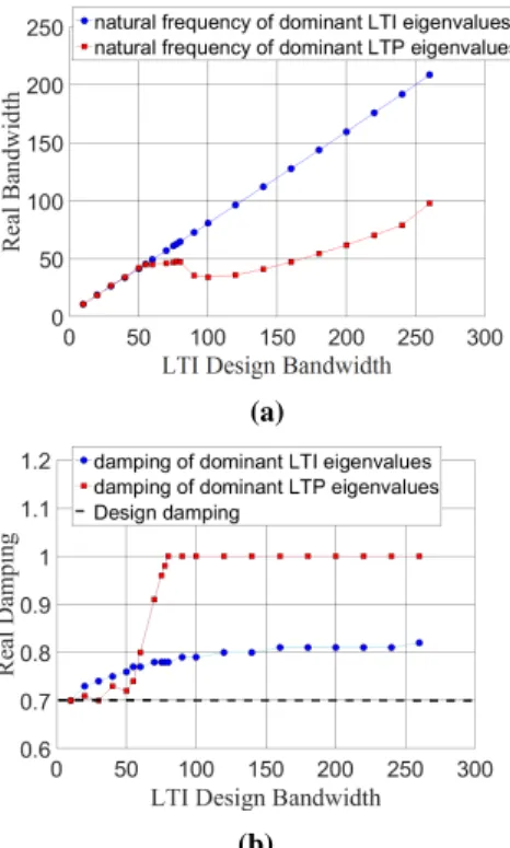
Fig. 6. (a) Design bandwidth versus actual bandwidth, blue circles - LTI model, red squares - LTP model; (b) design bandwidth versus damping, blue circles - LTI model, red squares - LTP model, dashed line - design damping.
Fig. 7. zoom 1 from Fig. 5, LTI and LTP eigenvalue loci-plot; black asterisks - LTI poles, red circles - LTP significant eigenvalues; eigenvalues associated with the notch filter.
in Fig. 5 for the set of control parameters recorded in Table II, corresponding to different LTI design bandwidths. Only dominant eigenvalues are reported, i.e. those that are closer to the imaginary axis and have smaller natural frequency.
From this plot, it can be seen that for an LTI design bandwidth Bw ≤ 55 Hz, the LTI and LTP eigenvalue loci-plots are consistent, whereas for Bw > 55 Hz the two plots become different and the actual eigenvalues of the system, those associated with the LTP model, move towards the real axis as the LTI design bandwidth increases. This analysis provides a range of validity for the LTI transfer function GV(s), calculated by applying the power balance
approach. In addition, Fig. 6 demonstrates that the actual bandwidth of the system follows the LTI design bandwidth up to55 Hz, then a further increase in the design bandwidth does not correspond to an increase of the real one. The LTI design damping for the closed-loop system is 0.7, whereas the LTP damping converges to unity for Bw > 75 Hz. The small difference between the LTI damping calculated using
W(s) (which converges to 0.8 for high Bw) and the LTI design damping is because the control design is based on
GV(s), while the closed-loop LTI poles are calculated based onF(s).
Observation: Fig. 5 and Fig. 6 can be used not only for analysis purposes, but also to design the voltage control above the limit of validity of the LTI model. It is possible to use a different pole-placement (for example LTP one) and then check the actual eigenvalues of the closed-loop system, thus its actual performance.
2) Stability boundaries of the DC voltage controller:
Now, taking into consideration Fig. 7, which shows zoom 1 from Fig. 5, and which represents the eigenvalues associated with the notch filter, the stability boundary of the actual system can be calculated. In general, increasingBwwill move these eigenvalues towards the imaginary axis, thus making the system less robust. It can be noticed that LTI and LTP approaches lead to different conclusions. Based on the LTI model, the system becomes unstable for Bw > 160 Hz, whereas from the LTP analysis the threshold isBw>240Hz, as also reported in Fig. 3. From simulation and experimental results it is found that the LTP threshold is correct, confirming that this approach provides more accurate results compared to traditional LTI methods.
Fig. 8.Small-signal time-domain analysis diagram.
B. Simulation Results
In order to provide a first validation of the eigenvalue loci plot of Fig. 5, a time-domain analysis based on small-signal injection is performed, as reported in Fig. 8. The small signal is provided by a10V step added to the reference voltage,Vref, and the small-signal output from the average model, as well as the outputs from the LTI and LTP models, are compared. In Fig. 9 these signals are recorded for a design bandwidth
Bw = 10 Hz of the voltage controller. As expected, a good match is achieved, meaning that both LTI and LTP models accurately describe the small-signal behaviour of the system. In Fig. 10 the LTI design bandwidth is increased toBw= 100
compared to that of the system, demonstrating that for high-bandwidth the LTP analysis provides more accurate results than an LTI one, and also providing a further validation of Fig. 5.
Fig. 9.Small-signal time-domain simulation withBw= 10Hz; blue
- small-signal reference, black - system response, red - LTI response, green - LTP response.
Fig. 10. Small-signal time-domain simulation withBw = 100 Hz;
blue - small-signal reference, black - system response, red - LTI response, green - LTP response.
The analytical results presented so far can be used either during the design process, in order to determine the limit of validity of approximated linearised models, hence to be able to obtain the maximum performance achievable by the actual system, or as a post-design stability assessment tool. In the first case, one can adjust the control parameters, in order to move the LTP eigenvalues to obtain a better-performing system, knowing that the LTP eigenvalues correspond to the actual eigenvalues of the system. In the second case, post-design stability assessment is recommended by using the LTP eigenvalue loci-plot.
More detailed simulations have been implemented in Matlab Simulink and Plecs, based on the switching model of the converter and control algorithm implemented in C language (including digital computational delay). A dead-time of3.6µs is also included. First the stability boundaries of the system are evaluated. This is done by starting the system with the first set of control parameters, as reported in Table II (Bw = 10
Hz), then these parameters are updated to the next set, corre-sponding to a higher LTI design bandwidth, until the stability threshold value is found.
(a)
(b)
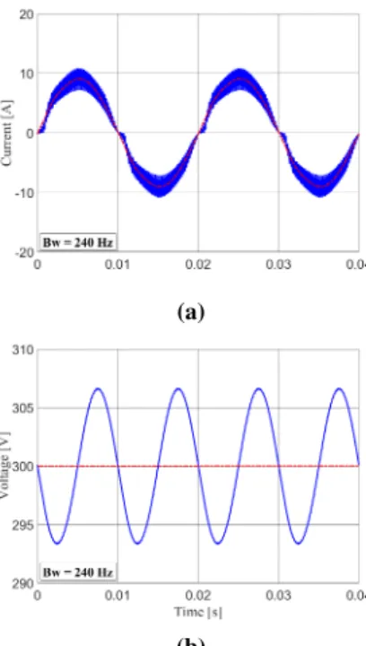
Fig. 11. Simulation data - (a) currents: blue - ig, red - iref; (b)
voltages: blue -vdc, red -Vref - stable system withBw= 240Hz.
(a)
(b)
Fig. 12.Simulation data - currents: blue - ig, red -iref; voltages:
blue -vdc, red -Vref; (a), (b), transition from a stable system with
Bw= 240Hz to an unstable system withBw= 260Hz (change at
t= 0s).
(a)
(b)
(c)
(d)
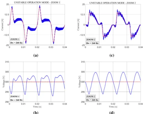
Fig. 13. Simulation data - currents: blue -ig, red -iref; voltages: blue -vdc, red -vref; unstable operation mode - (a), (b), zoom 1 of Fig.
12; (c), (d), zoom 2 of Fig. 12.
voltage control passes from Bw = 240Hz toBw = 260Hz, at t= 0. Since the unstable eigenvalues are very close to the imaginary axis, see Fig. 3 and Fig. 7, the unstable dynamics emerge very slowly. It can be seen that the current and voltage waveforms start to oscillate significantly after t = 5 s, and after t = 7 s the control no longer regulates the DC-link voltage. In Fig. 13 the simulation results of unstable operation are reported, with (a), (b), being the first zoom, and (c), (d),
being the second zoom in Fig. 12.
A second set of simulations is performed in order to assess the dynamic response of the system. A 50%load step is applied, i.e. a change of load from the nominal value
Rdc = 120 Ω to 60 Ω is made and the transient evolution of the grid current and DC-link voltage is recorded. In Fig. 14 the step load response is reported for Bw = 10 Hz in (a), (b), for Bw = 50 Hz in (c), (d), and for Bw = 100
(a)
(b)
(c)
(d)
(e)
(f)
Fig. 14.Simulation data for 50% load step transients - currents: blue -ig, red -iref; voltages: blue -vdc, red -vref; (a), (b), system with
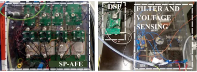
Fig. 16.10kW experimental setup.
Hz in (e), (f). In the voltage waveform are highlighted the maximum peak and the settling time, the latter being defined as the time required by the signal to reach2%error compared with the steady-state one. As it can be seen, increasing the LTI design bandwidth from 10Hz to 50Hz reduces both the voltage overshoots and the settling times. However, increasing the LTI design bandwidth further toBw= 100Hz leads on the one hand to smaller overshoots of the voltage waveform, but on the other hand to longer transients, which is in accordance with the analytical results.
C. Experimental Results
The experimental rig is a10kW 2-level IGBT inverter (con-trolled as a SP-AFE in this particular application) switching at fpwm = 10 kHz and with control algorithms and signal conditioning implemented in a custom DSP/FPGA board, Fig. 16. A double-update PWM is implemented, thus with control algorithm executed at twice the PWM frequency. No dead-time (tDT = 3.6 µs) compensation has been added to the control, in order to keep it as simple as possible. This explains the significant values of the current Total Harmonic Distortion (THD), which however does not affect the validity of the LTP
analysis, as it can be seen from the results below. The Power Factor (PF) is close to unity in all the control configurations, due to the fact that the current reference is generated by direct measurement of the grid voltage. The grid voltage is provided by a programmable AC source (Chroma).
The first set of experiments has been performed to validate the stability boundary of the system. In Fig. 15 the current and voltage waveforms are reported for both the stable and unstable operation mode, confirming the analytically calcu-lated stability threshold of Bw= 250 Hz. It can be seen that
the experimental case Bw = 240 Hz, Fig. 15(c), is slightly more distorted compared with the simulated one, Fig. 13(c), which is explained by the fact that the real system is more affected by noise.
The second set of experiments aims to validate the dynamic response of the system calculated analytically and confirmed by simulations. Hence, the simulation results highlighted in Fig. 14 are validated experimentally and reported in Fig. 17. It is thus confirmed that for a design bandwidthBw≤55Hz the system is well described by its LTI model, and the design specifications are met by the actual system; however a further increase ofBwmakes this assumption no longer correct. This can be observed by comparing the response of the system to load change for the case Bw = 100 Hz, where the latter exhibits a longer transient time and a smaller overshoot, in accordance to the analytical results reported in Fig. 6, where for an LTI design bandwidth of100Hz, the natural frequency of the dominant LTP eigenvalues is around40Hz.
VII. CONCLUSIONS
In this paper, the stability assessment for a single-phase active-front-end with fast DC voltage control loop is addressed
(a)
(b)
(c)
(d)
Fig. 15. Experimental data [5 ms/div] - currents: pink -ig; voltages: green - vdc; (a), stable system withBw= 10Hz, (c), stable system
withBw= 240Hz; (b), unstable system withBw= 260Hz, zoom 1 of Fig. 12; (d), unstable system withBw= 260Hz, zoom 2 of Fig.
(a)
(b)
(c)
(d)
(e)
(f)
Fig. 17. Experimental data for 50% load step transients [50 ms/div] - currents: pink -ig; voltages: green -vdc; (a)Bw = 10Hz step-up
load change, (b)Bw= 10Hz step-down load change, (c)Bw= 50Hz step-up load change, (d)Bw= 50Hz step-down load change, (e)
Bw= 100Hz step-up load change, (f)Bw= 100Hz step-down load change.
analytically exploiting LTP theory. It is shown that the conven-tional LTI analysis is valid only within the remit of the power-balance based approach. For this reason, the LTP approach is used first to determine the validity limits of the LTI models, and second to assess the actual stability of the overall system when fast voltage controllers are implemented. This leads to a mathematically more complex and detailed analysis. The superior results obtained using the LTP techniques, compared with those from the LTIs, are highlighted and validated by analytical, simulation and experimental results.
REFERENCES
[1] L. Malesani, L. Rossetto, P. Tenti, and P. Tomasin, “Ac/dc/ac pwm converter with reduced energy storage in the dc link,”IEEE Trans. Ind.
Appl., vol. 31, pp. 287–292, Mar 1995.
[2] R. M. Tallam, R. Naik, M. L. Gasperi, T. A. Nondahl, H. H. Lu, and Q. Yin, “Practical issues in the design of active rectifiers for ac drives with reduced dc-link capacitance,” in38th IAS Annual Meeting
on Conference Record of the Industry Applications Conference, 2003.,
vol. 3, pp. 1538–1545 vol.3, Oct 2003.
[3] P. Alemi, Y. C. Jeung, and D. C. Lee, “Dc-link capacitance minimiza-tion in t-type three-level ac/dc/ac pwm converters,”IEEE Trans. Ind.
Electron., vol. 62, pp. 1382–1391, March 2015.
[4] Y. Hu, Y. Du, W. Xiao, S. Finney, and W. Cao, “Dc-link voltage control strategy for reducing capacitance and total harmonic distortion in single-phase grid-connected photovoltaic inverters,”IET Power
Elec-tron., vol. 8, no. 8, pp. 1386–1393, 2015.
[5] W. J. Lee and S. K. Sul, “Dc-link voltage stabilization for reduced dc-link capacitor inverter,” in2009 IEEE Energy Conversion Congress and
Exposition, pp. 1740–1744, Sept 2009.
[6] X. Cao, Q. C. Zhong, and W. L. Ming, “Ripple eliminator to smooth dc-bus voltage and reduce the total capacitance required,”IEEE Trans.
Ind. Electron., vol. 62, pp. 2224–2235, April 2015.
[7] C. Rodriguez and G. A. J. Amaratunga, “Long-lifetime power inverter for photovoltaic ac modules,” IEEE Trans. Ind. Electron., vol. 55, pp. 2593–2601, July 2008.
[8] H. Wen, W. Xiao, X. Wen, and P. Armstrong, “Analysis and evaluation of dc-link capacitors for high-power-density electric vehicle drive systems,”
IEEE Trans. Veh. Technol, vol. 61, pp. 2950–2964, Sept 2012.
[9] M. Hinkkanen and J. Luomi, “Induction motor drives equipped with diode rectifier and small dc-link capacitance,”IEEE Trans. Ind.
Elec-tron., vol. 55, pp. 312–320, Jan 2008.
[10] R. Erickson and D. Maksimovic,Fundamentals of Power Electronics. Power electronics, Springer US, 2001.
[11] T. Isobe, D. Shiojima, K. Kato, Y. R. R. Hernandez, and R. Shimada, “Full-bridge reactive power compensator with minimized-equipped ca-pacitor and its application to static var compensator,”IEEE Trans. Power
Electron., vol. 31, pp. 224–234, Jan 2016.
[12] J. Kwon, X. Wang, F. Blaabjerg, C. Bak, A. Wood, and N. Watson, “Linearized modeling methods of ac-dc converters for an accurate frequency response,”IEEE J. Emerg. Sel. Top. Power Electron., vol. PP, no. 99, pp. 1–1, 2017.
[13] R. Wang, F. Wang, D. Boroyevich, R. Burgos, R. Lai, P. Ning, and K. Rajashekara, “A high power density single-phase pwm rectifier with active ripple energy storage,” IEEE Trans. Power Electron., vol. 26, pp. 1430–1443, May 2011.
[14] P. T. Krein, R. S. Balog, and M. Mirjafari, “Minimum energy and capacitance requirements for single-phase inverters and rectifiers using a ripple port,” IEEE Trans. Power Electron., vol. 27, pp. 4690–4698, Nov 2012.
[15] S. Qin, Y. Lei, C. Barth, W. C. Liu, and R. C. N. Pilawa-Podgurski, “Architecture and control of a high energy density buffer for power pulsation decoupling in grid-interfaced applications,” in2015 IEEE 16th
Workshop on Control and Modeling for Power Electronics (COMPEL),
pp. 1–8, July 2015.
[16] H. Hu, S. Harb, N. Kutkut, I. Batarseh, and Z. J. Shen, “A review of power decoupling techniques for microinverters with three different decoupling capacitor locations in pv systems,” IEEE Trans. Power
Electron., vol. 28, pp. 2711–2726, June 2013.
[17] D. G. Lamar, J. Sebastian, M. Arias, and A. Fernandez, “On the limit of the output capacitor reduction in power-factor correctors by distorting the line input current,”IEEE Trans. Power Electron., vol. 27, pp. 1168– 1176, March 2012.
[18] N. M. Wereley and S. R. Hall, “Frequency response of linear time periodic systems,” inDecision and Control, 1990., Proceedings of the
29th IEEE Conference on, pp. 3650–3655 vol.6, Dec 1990.
[19] S. R. Hall and N. M. Wereley, “Generalized Nyquist stability criterion for linear time periodic systems,” inAmerican Control Conference, 1990, pp. 1518–1525, May 1990.
[21] J. Kwon, X. Wang, F. Blaabjerg, C. L. Bak, V. S. Sularea, and C. Busca, “Harmonic interaction analysis in a grid-connected converter using harmonic state-space (hss) modeling,” IEEE Trans. Power Electron., vol. 32, pp. 6823–6835, Sept 2017.
[22] G. N. Love and A. R. Wood, “Harmonic state space model of power electronics,” in2008 13th International Conference on Harmonics and
Quality of Power, pp. 1–6, Sept 2008.
[23] E. Mollerstedt and B. Bernhardsson, “Out of control because of harmonics-an analysis of the harmonic response of an inverter loco-motive,”IEEE Control Syst. Mag., vol. 20, pp. 70–81, Aug 2000. [24] J. B. Kwon, X. Wang, F. Blaabjerg, C. L. Bak, A. R. Wood, and N. R.
Watson, “Harmonic instability analysis of a single-phase grid-connected converter using a harmonic state-space modeling method,”IEEE Trans.
Ind. Appl., vol. 52, pp. 4188–4200, Sept 2016.
[25] R. Z. Scapini, L. V. Bellinaso, and L. Michels, “Stability analysis of pfc ac-dc full-bridge converters with reduced dc-link capacitance,” IEEE
Trans. Power Electron., vol. PP, no. 99, pp. 1–1, 2017.
[26] V. Salis, A. Costabeber, P. Zanchetta, and S. Cox, “Stability analysis of single-phase grid-feeding inverters with pll using harmonic linearisation and linear time periodic (ltp) theory,” in2016 IEEE 17th Workshop on
Control and Modeling for Power Electronics (COMPEL), pp. 1–7, June
2016.
[27] S. Lissandron, L. D. Santa, P. Mattavelli, and B. Wen, “Experimental validation for impedance-based small-signal stability analysis of single-phase interconnected power systems with grid-feeding inverters,”IEEE
J. Emerg. Sel. Top. Power Electron., vol. 4, no. 1, pp. 103–115, March
2016.
[28] X. Wang, L. Harnefors, and F. Blaabjerg, “Unified impedance model of grid-connected voltage-source converters,”IEEE Trans. Power Electron., vol. 33, no. 2, pp. 1775–1787, Feb. 2018.
[29] T. Yang, S. Bozhko, J. M. Le-Peuvedic, G. Asher, and C. I. Hill, “Dy-namic phasor modeling of multi-generator variable frequency electrical power systems,”IEEE Trans. Power Syst., vol. 31, no. 1, pp. 563–571, Jan. 2016.
[30] S. Buso and P. Mattavelli, Digital Control in Power Electronics, 2nd
Edition. Morgan & Claypool, 2015.
[31] V. Salis, A. Costabeber, S. Cox, P. Zanchetta, and A. Formentini, “Stability boundary analysis in single-phase grid-connected inverters with pll by ltp theory,”IEEE Trans. Power Electron., vol. 33, pp. 4023– 4036, May 2018.
[32] V. Salis, A. Costabeber, S. M. Cox, and P. Zanchetta, “Stability assess-ment of power-converter-based ac systems by ltp theory: Eigenvalue analysis and harmonic impedance estimation,”IEEE J. Emerg. Sel. Top.
Power Electron., vol. 5, pp. 1513–1525, Dec. 2017.
[33] J. Sun and K. Karimi, “Small-signal input impedance modeling of line-frequency rectifiers,”IEEE Trans. Aerosp. Electron. Syst., vol. 44, pp. 1489–1497, Oct 2008.
[34] V. Salis, A. Costabeber, P. Zanchetta, and S. Cox, “A generalised har-monic linearisation method for power converters input/output impedance calculation,” in2016 18th European Conference on Power Electronics
and Applications (EPE’16 ECCE Europe), pp. 1–7, Sept 2016.
Valerio Salis(S’16 - M’18) received the Master’s degree with honours in Electronic Engineering from the University of Rome Tor Vergata, Rome, Italy, in 2014. He is currently working towards the Ph.D. degree in Electrical and Electronic Engineering in the Power Electronics, Machines and Control Group, University of Nottingham, Nottingham, UK. His research interests include study of instability issues in microgrids, linear time periodic system analysis and control design.
Alessandro Costabeber(S’09 - M’13) received the Degree with honours in Electronic Engineering from the University of Padova, Padova, Italy, in 2008 and the Ph.D. in Information Engineering from the same university in 2012, on energy efficient architectures and control techniques for the development of future residential microgrids. In the same year he started a two-year research fellowship with the same univer-sity. In 2014 he joined the PEMC group, Department of Electrical and Electronic Engineering, University of Nottingham, Nottingham, UK as Lecturer in Power Electronics. His current research interests include HVDC converters topologies, high power density converters for aerospace applications, control solutions and stability analysis of AC and DC microgrids, control and modelling of power converters, power electronics and control for distributed and renewable energy sources. Dr. Costabeber received the IEEE Joseph John Suozzi INTELEC Fellowship Award in Power Electronics in 2011.
Stephen M. Coxreceived the B.A. degree in mathe-matics from the University of Oxford, Oxford, U.K., in 1986, and the Ph.D. degree in applied mathemat-ics from the University of Bristol, Bristol, U.K., in 1989. He is currently a Reader in the School of Mathematical Sciences, University of Nottingham, Nottingham, U.K., where he was also a Lecturer and then a Senior Lecturer. From 2004 to 2006, he was a Senior Lecturer in the School of Mathematical Sciences, University of Adelaide, Australia. His re-search interests include the development of applied mathematical techniques for the modeling of class-D amplifiers and other power-electronic switching devices.
Andrea Formentiniwas born in Genova, Italy, in 1985. He received the M.S. degree in computer engi-neering and the Ph.D. degree in electrical engineer-ing from the University of Genova, Genova, in 2010 and 2014 respectively. He is currently working as research fellow in the Power Electronics, Machines and Control Group, University of Nottingham. His research interests include control systems applied to electrical machine drives and power converters.
![Fig. 17. Experimental data for 50% load step transients [50 ms/div] - currents: pink - i g ; voltages: green - v dc ; (a) B w = 10 Hz step-up](https://thumb-us.123doks.com/thumbv2/123dok_us/8561747.365845/11.918.97.820.81.443/fig-experimental-data-load-transients-currents-voltages-green.webp)
