An experimental study of hyper heuristic selection and acceptance mechanism for combinatorial t way test suite generation

1

An Experimental Study of Hyper-Heuristic Selection and Acceptance Mechanism for

Combinatorial t-way Test Suite Generation

KAMAL Z. ZAMLI and FAKHRUD DIN IBM Centre of Excellence

Faculty of Computer Systems and Software Engineering Universiti Malaysia Pahang

Lebuhraya Tun Razak, 26300 Kuantan, Pahang Darul Makmur, Malaysia Email: kamalz@ump.edu.my

GRAHAM KENDALL School of Computer Science University of Nottingham Malaysia Campus

Jalan Broga, 43500 Semenyih, Selangor Darul Ehsan, Malaysia Email: Graham.Kendall@nottingham.edu.my

BESTOUN S. AHMED Department of Computer Science Faculty of Electrical Engineering

Czech Technical University Karlovo n’am 13, 121 35 Praha 2, Czech Republic Email: bestoon82@gmail.com

Abstract

Recently, many meta-heuristic algorithms have been proposed to serve as the basis of a t-way test generation strategy (where t indicates the interaction strength) including Genetic Algorithms (GA), Ant Colony Optimization (ACO), Simulated Annealing (SA), Cuckoo Search (CS), Particle Swarm Optimization (PSO), and Harmony Search (HS). Although useful, meta-heuristic algorithms that make up these strategies often require specific domain knowledge in order to allow effective tuning before good quality solutions can be obtained. Hyper-heuristics provide an alternative methodology to meta-heuristics which permit adaptive selection and/or generation of meta-heuristics automatically during the search process. This paper describes our experience with four hyper-heuristic selection and acceptance mechanisms namely Exponential Monte Carlo with counter (EMCQ), Choice Function (CF), Improvement Selection Rules (ISR), and newly developed Fuzzy Inference Selection (FIS), using the t-way test generation problem as a case study. Based on the experimental results, we offer insights on why each strategy differs in terms of its performance.

Keywords: Software Testing; t-way Testing; Hyper-Heuristics; Meta-Heuristics; Fuzzy Inference Selection;

1. Introduction

Testing is an important process in software development to help identify areas where the software is not performing as expected. This process is often expensive owing to the time taken to execute the set of test cases. It has been a research focus to find suitable sampling strategies to generate a small yet efficient set of test cases for testing a software system.

2

Tackling this issue, and formulating interaction testing as an optimization problem, recent efforts have focused on the adoption of meta-heuristic algorithms as the basis for t-way testing strategy. Search Based Software Engineering (SBSE) [24], has developed many meta-heuristic based t-way strategies (e.g. based on Genetic Algorithms (GA) [14, 33], Particle Swarm Optimization (PSO) [4, 32, 45], Harmony Search (HS) [6], Ant Colony Optimization Algorithm (ACO) [14, 41], Simulated Annealing [17] and Cuckoo Search (CS) [2]), which have been reported in the scientific literature.

Meta-heuristic based strategies are known to produce a good quality t-way test suite. However, as suggested by the No Free Lunch theorem [44], the search for a single meta-heuristic that can outperform others in all optimization problem instances is fruitless. Hybridization of more than one meta-heuristic can be useful in enhancing the performance of t-way strategies, as hybridization can capitalize on the strengths and compensate the deficiencies of each individual algorithm.

Hybridization could be in the form of the integration of two or more search operators from different meta-heuristics, partly or in full, creating a new algorithm. Hybridization could also be an ensemble of two or more heuristics and running them sequentially or in parallel. Hyper-heuristics can also be viewed as a form of hybridization. Unlike the hybridization (including ensembles) of meta-heuristics, hyper-heuristics permit the integration of two or more meta-heuristic search operators from different meta-heuristics through one defined parent heuristic via non-domain feedback (i.e. (meta)-heuristic to choose (meta)-heuristics [10]). With a hyper-heuristic, the selection of a particular search operator to be used at any particular instance can be adaptively (and dynamically) decided based on the feedback from its previous performance.

In this paper, we explore the hybridization of meta-heuristics utilizing a hyper-heuristic approach. We present a new t-way testing strategy. In the context of our study, this paper focuses on an experimental study of hyper-heuristic selection and acceptance mechanism for adaptively selecting low-level search operators. Although there has been existing work (e.g. timetabling problems), this methodology has not been considered for t-way test generation as a case study. This paper describes our comparative studies with four hyper-heuristic selection and acceptance mechanisms namely Exponential Monte Carlo with counter (EMCQ) [9], Choice Function (CF) [20, 28], Improvement Selection Rules (ISR) [49], and the newly developed Fuzzy Inference Selection (FIS). These mechanisms utilize four common search operators comprising a Genetic Algorithm (GA) crossover search operator [25], Teaching Learning based Optimization (TLBO) algorithm’s peer learning search operator [39], Flower Algorithm’s global Pollination (FPA) search operator [48] and Jaya algorithm’s search operator [38].

The contributions of this paper can be summarized as follows:

• A new experimental study of existing hyper-heuristic selection and acceptance mechanisms, using t-way test generation as a case study. The study also benchmarks the results against existing meta-heuristic based strategies. Based on the results, we provide guidelines for choosing the appropriate mechanism and some insights on why each strategy differs in terms of performance.

• A new hyper-heuristic selection and acceptance mechanism based on Fuzzy Inference Selection (FIS).

The paper is organized as follows. Section 2 presents the theoretical framework covering the t-way test generation problem, its mathematical notation, related work as well as the main components of the hyper-heuristic. Section 3 describes the hyper-heuristic selection and acceptance mechanisms along with a description of each search operator. Section 4 presents our benchmarking experiments. Section 5 discusses our experimental observations. Finally, section 6 gives our concluding remarks along with the scope for future work.

2. Theoretical Framework

2.1. The t-way Test Generation Problem

Mathematically, the t-way test generation problem can be expressed by Equation 1.

𝑓𝑓(𝑍𝑍) = |{𝐼𝐼𝑖𝑖𝑖𝑖𝑉𝑉𝐼𝐼𝑉𝑉: 𝑍𝑍𝑐𝑐𝑐𝑐𝑐𝑐𝑐𝑐𝑐𝑐𝑐𝑐𝐼𝐼}| (1)

𝑆𝑆𝑆𝑆𝑆𝑆𝑆𝑆𝑐𝑐𝑐𝑐𝑆𝑆𝑆𝑆𝑐𝑐𝑍𝑍=𝑍𝑍1, 𝑍𝑍2, … , 𝑍𝑍𝑖𝑖𝑖𝑖𝑖𝑖𝑃𝑃1,𝑃𝑃2, … …𝑃𝑃𝑖𝑖; 𝑖𝑖= 1, 2, … , 𝑁𝑁

3

(Zi(1)<Zi(2)<……<Zi(K)); N is the number of decision variables (i.e. parameters); and K is the number of possible values for the discrete variables.

A simple configurable software system is used as a model to illustrate the t-way test generation problem. Figure 1 represents the topology of a modern e-commerce software system based on the Internet [3]. The system may use different components or parameters. In this example, the system comprises five parameters. The client side has two parameters or two types of clients: those who use smart phones and those who use normal computers. There are different configurations in both cases. On the other side are different servers and databases.

Figure 1. An E-commerce Software System [3]

The term “value” (i.e. v) is used to describe the configuration of each component. Thus, the system in Figure 1 can be summarized as a five-parameter system with a combination of three parameters with two values, and two parameters with three values, as in Table 1.

Table 1. An E- Commerce System Components and Configurations Components or Parameters

Payment Server

Smart Phone

Web Server

User Browser

Business Database

Configurations or Values

Master Card iPhone iPlanet Chrome SQL

Visa Card Blackberry Apache Explorer Oracle

Firefox Access

To reduce the risk and ensure the quality of such software, manufacturers may need to test all combinations of interactions (i.e. exhaustive testing), which requires 72 test cases (i.e. 2×2×2×3×3). However, testing of all combinations is practically impossible given large configurations or large components. Considering the pairwise (2-way) test generation for the E-commerce yields only 9 test cases (see Table 2). It should be noted that all the 2-way interaction tuples between parameters are covered at-least once.

Table 2. Pairwise Test Suite for E-Commerce System

Test No. Payment Server Smart Phone Web Server User Browser Business Database

1 Master Card Blackberry iPlanet Firefox Oracle

2 Visa Card iPhone Apache Firefox SQL

3 Master Card iPhone iPlanet Explorer Access

4 Visa Card Blackberry Apache Chrome Access

5 Visa Card iPhone iPlanet Chrome Oracle

6 Master Card Blackberry Apache Explorer SQL

7 Master Card iPhone iPlanet Chrome SQL

8 Visa Card iPhone Apache Explorer Oracle

4

2.2. The Covering Array Notation

In general, t-way testing has strong associations with the mathematical concept of Covering Arrays (CA). For this reason, t-way testing often adopts CA notation for representing t-way tests [42]. The notation CAλ (N;t,k,v) represents an array of size N with v values, such that every N×t sub-array contains all ordered subsets from the v values of size t at least λ times, and k is the number of components. To cover all t-interactions of the components, it is normally sufficient for each component to occur once in the CA. Therefore, with λ=1, the notation becomes CA (N;t,k,v). When the CA contains a minimum number of rows (N), it can be considered an optimal CA according to the definition in Equation 2.

𝐶𝐶𝐶𝐶𝑁𝑁(𝑆𝑆,𝑘𝑘,𝑐𝑐) = 𝑚𝑚𝑖𝑖𝑖𝑖{𝑁𝑁:Ǝ𝐶𝐶𝐶𝐶_𝜆𝜆(𝑁𝑁;𝑆𝑆,𝑘𝑘,𝑐𝑐)} (2)

To improve readability, it is customary to represent the covering array as CA (N;t,k,v) or simply CA(N;t,vk_). Considering CA (9; 2, 34_{) as an example, the covering array represents the strength of 2 with 4 parameters and 3}

values each. In the case when the number of component values varies, this can be handled by Mixed Covering Array (MCA), MCA(N;t,k,(v1,v2,…vk)) [16]. Similar to the covering array, the notation can be represented by MCA (N;t,k,vk_{). Using our earlier example of the E-commerce system in Figure 1, the test suite can be} represented as MCA (9; 2, 23₃2_).

2.3. Meta-Heuristic based t-way Strategies

The t-way test suite generation is an NP-hard problem [31] and significant research efforts have been carried out to investigate the problem. Computationally, the current approach can be categorized into one-parameter-at-a-time (OPAT) and one-test-at-a-one-parameter-at-a-time (OTAT) methods [35].

Derived from the in-parameter-order (IPO) strategy [31], the OPAT method begins with an initial array comprising of several selected parameters. The array is then horizontally extended until reaching all the selected parameters based on the required interaction coverage. This is followed by vertical extension, if necessary, to cover the remaining uncovered interactions. The iteration continues until all the interactions are covered.

Credited to the work of AETG [15], the OTAT method normally iterates over all the combinatorial interaction elements and generates a complete test case per iteration. While iterating, the strategy greedily checks whether the generated solution is the best fit value (i.e. covering the most uncovered interactions) from a list of potential solutions.

Adopting either the OPAT or the OTAT method, much effort has recently been focused on the use of meta-heuristic algorithms as part of the computational approach for t-way test suite generation. Termed Search based Software Engineering (SBSE), the adoption of meta-heuristic based strategies often produces more optimal test suite sizes although there may be tradeoffs in terms of computational costs.

Meta-heuristic based strategies can start with a population of random solutions. Then, one or more search operators are iteratively applied to the population in an effort to improve the overall fitness (i.e. in terms of greedily covering the interaction combinations). While there are many variations, the main difference between meta-heuristic strategies are the search operators. As far as the t-way test suite construction, meta-heuristics such as Genetic Algorithms (GA) [41], Ant Colony Optimization (ACO) [14], Simulated Annealing (SA) [18, 21], Particle Swarm Optimization (PSTG [4], DPSO [45], APSO [32]), Cuckoo Search (CS) [2] and Harmony Search Strategy (e.g. HSS) [6] have been reported in the scientific literature.

Each meta-heuristic algorithm has its own advantages and disadvantages. With hybridization, each algorithm can exploit the strengths and cover the weaknesses of the collaborating algorithms. Many recent results from the scientific literature (e.g. [22, 40]) seem to indicate that hybridization improves the performance of meta-heuristic algorithms.

5

2.4. Hyper-Heuristics and Related Work

Hyper-heuristics are alternative to meta-heuristics. Hyper-heuristics can be viewed as a high-level methodology which performs a search over the space formed by a set of low level heuristics which operate on the problem space. Unlike typical meta-heuristics, there is a logical separation between the problem domain and the high level hyper-heuristic. Apart from increasing the level of generality, hyper-heuristics can also be competitive with bespoke meta-heuristics.

Generally, hyper-heuristics can be classified as generative or selective [10]. Generative hyper-heuristics combine low-level heuristics to generate new higher level heuristics. Selective hyper-heuristics select from a set of low-level heuristics. Our work is based on selective hyper-heuristics. Selective hyper-heuristics can be online or offline. The former is unsupervised and learning happens dynamically during the search process, whilst the latter requires an additional training step prior to addressing the problem. For our work, we deal with online selective hyper-heuristics.

Owing to how the search process is undertaken, the aforementioned hyper-heuristic classification (i.e. selective or generative) can further be extended to either perturbative or constructive [10]. Perturbative heuristics (also known as improvement heuristics) manipulate complete candidate solutions by iteratively changing their component(s). In the case of selection methodologies, perturbative hyper-heuristics provide a combination of low-level meta-heuristic operators and/or simple heuristic searches with the aim of selecting and applying them for the improvement of the current solution. Some problems addressed with such hyper-heuristics are vehicle routing [40], project scheduling [8], timetabling [11], GA parameter tuning [23], and CAs construction [27, 49].

Constructive hyper-heuristics process partial candidate solutions by iteratively extending missing element(s) to build complete solutions. As a selection methodology, this approach combines several pre-existing low-level constructive meta-heuristic operators, selecting and using the (perceived) best heuristic for the current problem state. Combinatorial optimization problems such as production scheduling [13], cutting and packing [43], and timetabling [7] have been successfully addressed with this approach.

In the context of the current study, some previous hyper-heuristics research is particularly relevant. Choice Function (CF) and Exponential Monte Carlo with Counter (EMCQ) [9] are among the earliest hyper-heuristics reported in the scientific literature. CF exploits the reinforcement learning framework to penalize and reward (meta)-heuristics through a set of choice functions (f1, f2, f3). The first parameter f1 relates to the effectiveness of the currently employed heuristic. The second parameter f2 evaluates the effectiveness of two heuristics when used consecutively. The third parameter f3 increases the probability of a heuristic being selected, over time, to encourage exploration. EMCQ adopts a simulated annealing like probability density function that is a function of the number of iterations. A worsening fitness causes EMCQ to decrease its acceptance probability. Both CF and EMCQ are further discussed in the next section.

With regard to the use of a fuzzy inference system, as part of a hyper-heuristic, Asmuni et al. [7] developed a constructive hyper-heuristic for addressing the timetabling problem. In their work, the Mamdani type fuzzy system is responsible for scheduling courses based on the perceived difficulty. Different orderings are considered, for example, the event with the highest crisp value (most difficult) is scheduled first. Recently, Gudino-Penaloza et al. [23] developed a new hyper-heuristic using a Takagi-Sugeno based fuzzy inference system to adaptively adjust the control parameters of a GA. Although using fuzzy inference system, the works of both Asmuni et al. and Gudino-Penaloza et al. have a slightly different focus. Specifically, our work deals with heuristic selection and not event ordering or adaptive meta-heuristic parameter control adjustment.

As far as the t-way test suite generation problem is concerned, the work of Jia et al. [27] can be considered the pioneering effort to investigate the usefulness of hyper-heuristics for t-way test generation. Similar to EMCQ, the work adopts a simulated annealing based hyper-heuristic, called HHSA, to select from variants of six operators (i.e. single/multiple/smart mutation, simple/smart add and delete row). HHSA demonstrates good performance in terms of test suite size as well as displaying elements of learning in the selection of the search operators.

6

the search operators. Additionally, it also incorporates lightweight search operators to minimize computational resources.

3. The Hyper-Heuristic Selection and Acceptance Mechanism

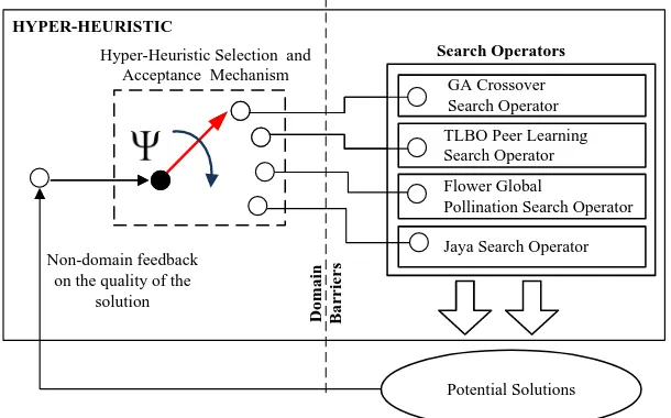
The selection and acceptance mechanism for selection based heuristics is shown in Figure 2. The hyper-heuristic selection and acceptance mechanism is represented by the dashed rectangle.

Non-domain feedback on the quality of the

solution

GA Crossover Search Operator

TLBO Peer Learning Search Operator

Potential Solutions Hyper-Heuristic Selection and

Acceptance Mechanism

Search Operators

Domain Barriers HYPER-HEURISTIC

Flower Global Pollination Search Operator

Jaya Search Operator

Figure 2. The Hyper-Heuristic Selection and Acceptance Mechanism

We compare the performance of Exponential Monte Carlo with counter (EMCQ), Choice Function (CF), Improvement Selection Rules (ISR) and the newly developed Fuzzy Inference Selection (FIS) as the selection and acceptance mechanism. We use four common search operators comprising of a GA crossover operator, a TLBO peer learning search operator, an FPA global pollination search operator and Jaya algorithm’s search operator.

The selection of the search operators needs to take into account the balance between diversification and intensification. As such, any arbitrary (but balanced) selection of the search operators is also possible. In our case, the FPA global pollination and the Jaya algorithm serve as the global search operators. The GA crossover and the TLBO peer learning serve as the local search operators.

3.1 Description of the Selection and Acceptance Mechanism

The next subsections detail the selection and acceptance mechanisms.

3.1.1 The Exponential Monte Carlo with Counter

The Exponential Monte Carlo with Counter (EMCQ) is a parameter free hyper-heuristic developed by Ayob and Kendall [9]. EMCQ probabilistically accepts lesser quality solutions (similar to simulated annealing [30]) in order to escape from local optima. In EMCQ, the probability density is defined in Equation 3 as:

Ψ=𝑐𝑐−𝛿𝛿∗𝑇𝑇/𝑞𝑞 (3)

where δ is the difference in fitness value between the current solution (Si) and the previous solution (S0) (i.e. δ=

f(Si) – f(S0)), t is the iteration counter, and q is a control parameter for consecutive non-improving iterations.

7

Referring to the pseudo code of EMCQ in Figure 3, line 1 initializes the populations of the required t-way interactions, I = {I1, I2… IM}. The value of M depends on the given inputs interaction strength (t), parameter (k) and its corresponding value (v). Specifically, M captures the number of required interactions that needs to be captured in the constructed covering array. Mathematically, M can be obtained as the sum of products of each individual’s t-wise interaction. For example, for CA (9;2, 34_{), M takes the value of 3x3+3x3+3x3+3x3+3x3+3x3}

= 54. If MCA (9; 2, 32 ₂2_{) is considered, then M takes the value of 3x3+3x2+3x2+3x2+3x2+2x2= 37. Line 2}

defines the maximum iteration ϴmax and population size, S. Line 3 randomly initializes the initial population of solutions Z = {Z1, Z2… ZN}. Line 4 selects the random initial search operator, H0. Line 5 applies H0 to generate initial solution, S0. Line 6 sets Sbest = S0as an initial value and Hi=H0 as the initial search operator. The main loop starts in line 7 and will iterate until the coverage of all interaction tuples (I). Line 8 assigns 1 to variable T which acts as a loop counter. The inner while loop starts in line 9 with ϴmax as the maximum number of iterations. Line 10 applies the current Hi to produce best Si to be added in the final test suite, Fs. Line 11 computes the fitness difference, δ = f(Si) – f(Sbest). In lines 12-15, if the fitness improves (i.e. δ > 0), Hiis kept for the next iteration. Here, q is reset to 1 in line 14 (i.e. because the fitness improves). Line 17 computes the probability density,Ψ. In line 18, upon a poor move, the solution might be accepted based on the probability density Ψ. If accepted, Hi is kept and q is reset to 1 (as in lines 19-21), otherwise, Hi is changed and q is incremented by 1 (see lines 23-25). Lines 27-28 update the values of Sbest and T for the next iteration. If there

are uncovered t-wise interaction, the mentioned procedure is repeated again until termination.

Figure 3. Pseudo Code for EMCQ

8

The Choice Function (CF), termed Choice Function Accept All Moves, was first proposed by Kendall et al.[28]. Based on the reward and punish approach, CF utilizes the choice function (F) to select from a set of low level heuristics. The corresponding values of F are calculated and updated for each individual low level search operator during execution. In our implementation, we adopt the variant of the choice function implementation by Drake et al. [20]; the Modified Choice Function.

Similar to the original choice function implementation, the calculation of F depends on three parameters f1,f2, and f3. Parameter f1measures the effectiveness of the currently employed search operator hi. The value of f1for a particular search operator is evaluated using Equation 4:

𝑓𝑓₁(𝐻𝐻_𝑖𝑖) =𝐼𝐼((𝑆𝑆_𝑖𝑖(𝐻𝐻_𝑖𝑖))/𝑇𝑇(𝐻𝐻_𝑖𝑖) +𝜙𝜙𝑓𝑓₁(𝐻𝐻_𝑖𝑖) (4)

where I(S_𝑖𝑖(H𝑖𝑖) is the change in solution fitness produced by hi, T(H𝑖𝑖) is the time taken by the search operator hi, and ϕ is a parameter from the interval (0,1) which gives greater importance to the heuristic’s recent performance.

Parameter f2 (Hi,Hj) measures the effectiveness of the current search operator hi when employed immediately following hj. The value of f2 is computed using Equation 5.

𝑓𝑓₂(𝐻𝐻_𝑖𝑖,𝐻𝐻_𝑗𝑗) =𝐼𝐼((𝑆𝑆_𝑖𝑖(𝐻𝐻_𝑖𝑖), (𝑆𝑆_𝑗𝑗(𝐻𝐻_𝑗𝑗))/𝑇𝑇�𝐻𝐻_𝑖𝑖,𝐻𝐻_𝑗𝑗� +𝜙𝜙𝑓𝑓₂(𝐻𝐻_𝑖𝑖,𝐻𝐻_𝑗𝑗) (5)

where I((S_𝑖𝑖(𝐻𝐻_𝑖𝑖),(S_𝑗𝑗(H𝑗𝑗)) is the change in fitness of hi and hj, T (Hi, Hj) is the time taken by both the heuristics and ϕ is same as in f1.

Parameter f3 captures the time elapsed since the search operator hk had been called. The parameter f3 is computed using Equation 6:

𝑓𝑓₃(𝐻𝐻_𝑘𝑘) =𝜏𝜏(𝐻𝐻_𝑘𝑘) 𝑤𝑤ℎ𝑐𝑐𝑐𝑐𝑐𝑐𝑘𝑘= 0 𝑆𝑆𝑐𝑐𝑁𝑁 −1 (6)

where N is equal to the total number of available operators.

Using the calculated f1,f2, and f3 values, the Modified Choice Function F gives a score to each search operator in order to select the best one based on Equation 7.

𝐹𝐹_𝑡𝑡(𝐻𝐻_𝑖𝑖) =𝜙𝜙𝑓𝑓₁(𝐻𝐻_𝑖𝑖) + 𝜙𝜙𝑓𝑓₂(𝐻𝐻_𝑖𝑖,𝐻𝐻_𝑗𝑗) + 𝛿𝛿𝑓𝑓₃(𝐻𝐻_𝑖𝑖) (7)

where t represents the current invocation.

Following the recommendation by Drake et al. [20], the values ofϕ and δ are initially set at 0.5. If the solution fitness improves in any iteration, ϕ is given the highest value of the interval (0, 1) whereas δ is given the lowest value. In case of a low-quality solution, the value of ϕ is decreased by 0.01 and the value of δ is automatically increased (see Equation 9). This leads to the diversification of the heuristic search process. The settings make the intensification factor prominent in the evaluation of F. For each iteration, the values of ϕt and δt in the

Modified Choice Function are calculated as shown in Equations 8 and 9:

𝜙𝜙_𝑡𝑡=

�_{𝑚𝑚𝑞𝑞𝑚𝑚}0.99, _{𝜙𝜙 𝑖𝑖𝑓𝑓𝑞𝑞𝑆𝑆𝑞𝑞𝑞𝑞𝑖𝑖𝑆𝑆𝑞𝑞𝑖𝑖𝑚𝑚𝑖𝑖𝑐𝑐𝑐𝑐𝑐𝑐𝑐𝑐𝑐𝑐

𝑡𝑡−1−0.01,0.01} , 𝑖𝑖𝑓𝑓𝑞𝑞𝑆𝑆𝑞𝑞𝑞𝑞𝑖𝑖𝑆𝑆𝑞𝑞𝑑𝑑𝑐𝑐𝑆𝑆𝑐𝑐𝑐𝑐𝑖𝑖𝑐𝑐𝑐𝑐𝑞𝑞𝑆𝑆𝑐𝑐𝑐𝑐

(8)

𝛿𝛿𝑡𝑡= 1− 𝜙𝜙𝑡𝑡

(9)

9

Lines 1-3 perform the necessary initialization related to the t-way problem (similar to the case of EMCQ). Line 4 initializes the value of ϕ and δ. Line 5 randomly selects any meta-heuristic Hi to produce an initial solution Si. The initial values for the three measures f1, f2, and f3are computed (6-8). Line 9 sets the current heuristic Hi to last heuristic Hj. The main loop starts in line 10 and will iterate until the coverage of all interaction tuples (I). Line 11 assigns 1 to variable T which acts as a loop counter. The inner while loop starts in line 12 with ϴmax as the maximum number of iterations. The marking of the heuristics for selection begins in line 13 with the computation of the Modified Choice Function F. Line 14 applies the search operator which maximizes F. The best Si is added to the final test suite, Fs.The computation of the three measures is performed in lines 15-17. If the solution fitness improves (i.e. I((S_𝑖𝑖(𝐻𝐻_𝑖𝑖)≥ 0)) the values of ϕ and δ are set to 0.99 and 0.01 (in lines 19-20) respectively. In line 21, the solution fitness of the last heuristic, Hj is also computed. In the case of a poor fitness, ϕ is decreased linearly (lines 24-25) and the new value for δ asδ = 1 - ϕ is computed in line 27. The solution fitness of the current heuristic is set to 0.00 (line 28) as it is poor. Lines 30-31 update Hj and T for the next iteration.

Figure 4: Modified Choice Function

3.1.3 Improvement Selection Rules

10

checks for improvements in the objective function. The diversification operator measures how diverse the current and the previously generated solutions are against the population of potential candidate solutions. Finally, the intensification operator evaluates how close the current and the previously generated solution are against the population of solutions. Apart from its three operators, ISR also exploits a Tabu List to penalize its poorly performing heuristics. Figure 5 summarizes the pseudo code for ISR.

Figure 5. Improvement Selection Rules

Lines 1-3 perform the t-way problem initialization (similar to the EMCQ and the choice function described earlier). Lines 4-5 select H0 randomly to produce S0 from the four available meta-heuristics. The main loop starts in line 6 and will iterate until the coverage of all interaction tuples (I). Line 7 assigns 1 to variable T which acts as a loop counter. The inner while loop starts in line 8 with ϴmax as the maximum number of iterations. In line 9, Hi is summoned to produce the best Sito be added to the final test suite, Fs. To decide whether to select a new LLH or not, the three operators, comprising the improvement, diversification and intensification (lines 10-12) will be used. The improvement operator compares the current Siagainst the previous Si-1 from the final test suite Fs. F1 evaluates to true only if Si ≥ previous Si-1. The diversification operator exploits the hamming distance measure to evaluate the diversification of each Si solution (i.e. in terms of how far Si is from the population of candidate solutions). Like the diversification operator, the intensification operator also exploits the hamming distance to evaluate the intensification of each previous S solution. Unlike the diversification operator, the intensification operator measures the intensification value, Iv, of Si against the final test suite Fs population (i.e. how close is Sbest to the final test suite). To be more specific, the intensification value can be defined as the cumulative sum of the hamming distance of each individual Fs population with Si. Here, the current value of Iv will be compared to the previous value of Iv (i.e. from the previous iteration). F3 evaluates to true only if the

current Iv ≤ the previous Iv.

In line 13, the selection and acceptance mechanism, Ψ (Hi, F1, F2, F3) evaluates to true, if and only if, F1 = true

and F2 = true and F3 = true. If Ψ (Hi, F1, F2, F3) evaluates to false, the new Hi will be selected (and the current

11

Referring to lines 18-22, the current Hiis penalized and will miss at least one turn from being selected in the next iteration. Apart from one’s own performance in terms of objective value improvement, diversification, and intensification, a particular search operator can be chosen more frequently than others owing to the random selection of search operators within the Tabu List (line 19).

3.1.4 Fuzzy Inference Selection

Finding the right fuzzy membership estimation is actually a very challenging process (as the only restriction that a membership function has to satisfy is its value be in [0,1] range). Design choices are often problem dependent, hence, cannot be easily generalized. Literature [36] suggests at least three approaches for membership function estimation (i.e. expert-driven approaches via knowledge acquisition from experts, data-driven approaches via structuralisation of data, and principle of justifiable granularity via information granularity in terms of sufficient experimental evidence and high specificity). In our current work, we have adopted the variant of expert-driven (as we have exploited existing knowledge on the fuzzy inference as well as on our problem domain).

A number of design choices are relevant in the implementation of the proposed Fuzzy Inference Selection (FIS) as follows:

• Mamdani with triangular/trapezoidal membership – As fuzzy rules can be expressed as linguistic constraints that are easy to understand and maintain, Mamdani inference is preferred over Sugeno. Furthermore, previous studies which combine fuzzy and meta-heuristics often favor Mamdani inference. In fact, the majority of these studies used Mamdani inference with centroid defuzzification and implemented either triangular/trapezoidal or Gaussian membership function. Empirical analysis using both types of membership functions showed that triangular/trapezoidal membership functions gave better performance over Gaussian ones [12, 19]. Therefore, in this study, the fuzzy inference system that uses Mamdani type inference with triangular/trapezoidal membership function and centroid defuzzification has been chosen for our implementation.

• Membership cardinality, fuzzy rules and normalization – The proposed FIS as the search operator selection and acceptance mechanism is derived from our earlier work on ISR described in [49]. Like ISR, FIS adopts three operators (i.e. improvement, diversification intensification) based on a Hamming distance measure. Recall that the improvement operator checks for improvements in the quality of the objective function. The diversification operator measures how diverse the current and the previously generated solutions are against the population of potential candidate solutions. Finally, the intensification operator evaluates how close the current and the previously generated solutions are against the population of solutions. Based on the three defined operators, we propose three membership functions representing input for each operator. Owing to its origin, the FIS fuzzy rules have been designed based on the ISR Boolean logic. However, unlike ISR which uses strict Boolean logic, the proposed FIS also accepts partial truth (i.e. based on some degree of membership) allowing more objective control to maintain or potentially change any particular search operator during runtime. In this case, the operator selection is set as the output variable. Concerning normalization of input and output values, we exploit our knowledge on the maximum possible hamming distance range based on the specified input parameters and its values.

• Linguistic terms and their overlapping functions – We have chosen three overlapping (and equal-width) linguistic terms for all membership functions between the multiple interval ranges of 0, 25, 50, 75 and 100. The choice for the number of linguistic terms can be seen as two sides of the same coin. Too many linguistic terms invite more rules, hence, potentially introduce more elaborate computations (and it also affects the widths and the interval ranges). Too little linguistic terms hinder good decision making. As our application involves non-intricate fuzzy decision making, we foresee three linguistic terms for inputs and two linguistic terms for output are sufficiently adequate. Concerning overlapping, we have adopted the work of Mizumoto [34] which suggests that overlapping linguistic terms must start at their center points, where the performance of the fuzzy system is at best (i.e. considering completely non-overlapping of linguistic terms may not fire any rules given out-of-range input values).

12

OUTPUT MEMBERSHIP

FUZZY INFERENCE SELECTION

Maintain Selection Rules

RULE 1 : IF Quality IS Excellent AND Diversification IS Excellent AND Intensification IS Excellent

THEN Selection IS Maintain;

May Change Selection Rules

RULE 2 : IF Quality IS Excellent AND Diversification IS Excellent AND Intensification IS Good

THEN Selection IS May_Change;

RULE 3 : IF Quality IS Excellent AND Diversification IS Good AND Intensification IS Excellent

THEN Selection IS May_Change;

RULE 4 : IF Quality IS Good AND Diversification IS Excellent AND Intensification IS Excellent

THEN Selection IS May_Change;

Change Selection Rules

RULE 5 : IF Quality IS Poor THEN Selection IS Change; RULE 6 : IF Diversification IS Poor THEN Selection IS Change; RULE 7 : IF Intensification IS Poor THEN Selection IS Change;

RULE 8 : IF Quality IS Good AND Diversification is Good AND Intensification IS Good

THEN Selection IS Change; FUZZY RULES CRISP OUTPUT Centroid DEFUZZIFIER Intensification Measure Quality Measure INPUT MEMBERSHIP Diversification value Intensification value Quality value CRISP INPUTS 0.00 0.25 0.50 0.75 1.00 10

0 20 30 40 50 60 70 80 90 100 Good Excellent Poor

Degree of _Membership

Diversification Measure Normalized Percentage Inputs 0.00 0.25 0.50 0.75 1.00 10

0 20 30 40 50 60 70 80 90 100 Good Excellent Poor

Degree of _Membership

Normalized Percentage Inputs Normalized Percentage Inputs 0.00 0.25 0.50 0.75 1.00 Good Poor Excellent

Degree of _Membership

10

0 20 30 40 50 60 70 80 90 100

0.00 0.25 0.50 0.75 1.00 10

0 20 30 40 50 60 70 80 90 100 May

Change Maintain Change

Degree of _Membership

Operator Selection

Output

Figure 6. Fuzzy Inference Selection

The block, labeled INPUT MEMBERSHIP takes the crisp values of the three operators and fuzzifies them. The fuzzification process is based on three defined triangular/trapezoidal membership functions with linguistic terms namely Poor, Good and Excellent. It is worth noting that the triangular/trapezoidal membership functions for the diversification operator and improvement operator are identical. The values in the range of 0-50 are considered Poor. The values in the range of 25-75 are considered Good and the values in the range of 50-100 are considered Excellent. In the case of the intensification operator, the Excellent range and the Poor range are swapped (i.e. Excellent range is defined from 0-50 whilst the Poor range is defined from 50-100). There is no change as far as the Good range is concerned.

Given the defined membership functions and based on the parameter inputs (i.e. interaction strength (t), parameter (k) and its corresponding value (v)), each of the crisp input from each operator need to undergo normalized scaling to fit in the defined percentage range. In general, the normalized values are computed as follows (based on Equation 10):

𝐹𝐹_{𝑠𝑠𝑠𝑠𝑠𝑠𝑠𝑠𝑠𝑠𝑠𝑠}= (𝐹𝐹_{𝑠𝑠𝑠𝑠𝑡𝑡𝑎𝑎𝑠𝑠𝑠𝑠}∗100)/(𝐹𝐹_{𝑚𝑚𝑠𝑠𝑚𝑚}) (10)

The Fmax value depends on the operator. Concerning the diversification operator, the Fmax corresponds to the maximum diversity possible (i.e. all the values within inputs are completely changed). For this reason, Fmax is always equal to the input parameter (k). As for the intensification operator, Fmax corresponds to the maximum intensification possible (i.e. again with all the values within inputs are completely changed). As such, Fmax for the intensification operator is also always equal to the input parameter (k). Contrary to this, Fmax calculation is different for the improvement operator. Here, Fmax corresponds to the maximum possible interaction coverage given as input parameter (k) and interaction strength (t). Specifically, Fmax for the improvement operator can be mathematically defined by Equation 11.

13

For the OUTPUT MEMBERSHIP block, a single output operator called Selection is defined. The Selection operator has three linguistic terms called Change, May Change, and Maintain represented by the triangular/ trapezoidal membership function (similar to intensification and diversification operators) taking the ranges of 0-50, 25-75 and 50-100 respectively.

The FUZZY RULES block lists the linguistic rules of FIS. The total number of rules r for a fuzzy system is determined by Equation 12.

𝑐𝑐 = ∏ 𝑓𝑓_𝑖𝑖𝑁𝑁 _𝑖𝑖 (12)

where N is the total number of crisp inputs and fiis the number of terms for each input variable.

In our case, there are potentially 33 _{or 27 rules for the FIS (as each operator takes three linguistic terms). Based}

on our observation, the rules can be reduced to 8 rules as shown in Figure 6. Specifically, the selection of the search operator will not be changed (i.e. Maintain) if all three operators’ values are evaluated as Excellent. The search operator may be changed (i.e. May Change) if any of the two operators’ values are Excellent and the third value is Good. FIS changes (i.e. Change) the search operator for the next iteration if any one of the operators is Poor or all operators are Good.

Finally, the Fuzzy Inference Selection aggregates the reasoning and takes fuzzy actions in light of input/output memberships, linguistic variables and fuzzy rules. The fuzzy results are then forwarded to the DEFUZZIFIER block. This block translates the fuzzy results into crisp output using the Center of Gravity, based on the defined DEFUZZIFIER block in order to produce crisp values for the control variables (see Equation 13).

𝑈𝑈= ∫ 𝑈𝑈𝜇𝜇 (𝑈𝑈) 𝑠𝑠𝑈𝑈

𝑀𝑀𝑀𝑀𝑀𝑀 𝑀𝑀𝑀𝑀𝑀𝑀

∫_{𝑀𝑀𝑀𝑀𝑀𝑀}𝑀𝑀𝑀𝑀𝑀𝑀𝜇𝜇 (𝑈𝑈) 𝑠𝑠𝑈𝑈

Summing up, Figure 7 summarizes the complete FIS pseudo code.

14

Figure 7. Fuzzy Inference Selection

Lines 1-3 perform t-way problem initialization similar to the earlier described hyper-heuristics. The maximum operator value, F_Max, is computed in line 4. Line 5 defines the fuzzy rules used by the FIS. The main loop starts in line 6 which repeats the necessary steps until the coverage of all interaction tuples (I). Line 7 sets variable T to value 1. The inner loop starts in line 8 that runs for ϴmax. Line 9 selects Hi in order to produce a solution Si and add it to Fs. Lines 10-12 compute the values of the three operators (i.e. improvement F1, diversification F2, as well as intensification F3). These values will be utilized for the fuzzy based selection of Hi. Line 13 computes the scaled value for each operator Fi as Fscaled as Fscaled = (Factual×100)/Fmax . Lines 14-17, encompass the FIS logic. In line 14, the scaled value of each operator and the Selection output variable are translated into linguistic terms with trapezoidal membership functions (as depicted in the INPUT/OUTPUT MEMBERSHIP blocks in Figure 6). FIS, in line 15, combines all the fuzzy information for the DEFUZZIFIER block. The defuzzifier produces the crisp output in Line 16. Line 17 assigns the crisp output to the Selection variable. In lines 18-25, the fuzzy inference selection will decide, based on the Selection value, whether to maintain, change or may change the heuristic Hifor the next iteration. In case, the operator is found Poor (lines 18-19), the current Hi will be replaced in the next iteration. When the Selection variable is in range (Selection > 40.0 and ≤ 60.0), the current Himay or may not be changed for the next iteration (lines 21-22). FIS keeps the current Hi (line 24) for the next iteration if the Selection variable is greater than 60. Line 26 updates T for the next iteration.

3.2 Description of the Search Operators

The next subsections provide the description of the adopted search operators.

15

The crossover search operator is derived from the Genetic Algorithm [25]. The complete algorithm is defined in Figure 8. Initially, Sbest is set to Z0 in line 1. The loop starts in line 2. The crossover operation occurs between a randomly selected Zi against the existing Zi in the population over the randomized length (α) (in lines 3-5). If the newly updated Zihas a better fitness value, the value of Zi is updated accordingly (in lines 6-7). The fitness of the current Zi is checked against Sbest. Sbestwill be updated if it has better fitness than Zi (in lines 9-10).

Figure 8. GA Crossover Search Operator

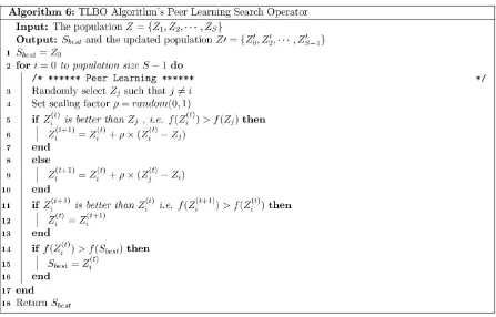
3.2.2 Teaching Learning based Optimization Peer Learning Search Operator

As the name suggests, the TLBO peer learning search operator is derived from the learning phase of the Teaching Learning based Optimization Algorithm [39]. The algorithm was originally proposed as a local search operator. Figure 9 presents the complete algorithm.

16

Figure 9. TLBO Algorithm’s Peer Learning Search Operator

3.2.3 Flower Pollination Algorithm Global Pollination Operator

The FPA global pollination search operator is derived from the Flower Pollination Algorithm [48]. The global pollination operator exploits Lévy Flight motion to update all the (column-wise) values for Ziof interest instead of only perturbing one value, thus, making it a global search operator. The complete algorithm is summarized in Figure 10.

Considering the flow of the global pollination operator, Sbest is initially set to Z0 in line 1. The loop starts in line 2. The value of Zi will be iteratively updated using the transformation equation exploiting the Lévy Flight motion (in lines 4-6). The Lévy Flight motion is a random walk that takes a sequence of jumps, which are selected from a heavy tailed probability function. For our Lévy Flight implementation, we adopt the well-known Mantegna’s algorithm [47]. Within this algorithm, a step length can be defined as (See Equation 14):

𝑆𝑆𝑆𝑆𝑐𝑐𝑖𝑖= 𝑎𝑎

[𝑣𝑣]1𝛽𝛽

(14)

where 𝑆𝑆 and 𝑐𝑐 are approximated from the normal Gausian distribution in which:

𝑆𝑆 ≈ 𝑁𝑁(0,𝜎𝜎_𝑎𝑎2) ∙ 𝜎𝜎_𝑎𝑎 𝑐𝑐 ≈ 𝑁𝑁(0,𝜎𝜎_𝑣𝑣2)∙ 𝜎𝜎_𝑣𝑣

(15)

For 𝑐𝑐 value estimation, we use 𝜎𝜎_𝑣𝑣 = 1. For 𝑆𝑆value estimation, we evaluate the Gamma function(

ᴦ

𝜎𝜎_𝑎𝑎= �

ᴦ

𝜋𝜋𝛽𝛽

2 �

ᴦ

1 𝛽𝛽

(16)

In our case, the Gamma function(ᴦ) implementation is adopted from William et al. [37].

17

Figure 10. Flower Algorithm’s Global Pollination Operator

3.2.4 Jaya Algorithm’s Search Operator

The Jaya search operator is derived from the Jaya algorithm [38]. The complete description of the Jaya operator is summarized in Figure 11.

Unlike the search operators described earlier (i.e. keeping track of only Sbest), the Jaya search operator keeps track of both Sbest and Spoor. As seen in line 6, the Jaya search operator exploits both Sbest and Spoor as part of its transformation equation. Although biased towards global search, the transformation equation can also address local search. In the case when ΔS= Sbest -Spooris sufficiently small, the transformation equation offset (in line with the term

ʊ

As far as the flow of the Jaya operator is concerned, lines 1-2 sets up the initial values for Sbest = Z0 and Spoor =

18

Figure 11. Jaya Search Operator

4. The Experiments

Our experiments focus on three related goals: (1) to characterize the performance of the implemented heuristic with each other; (2) to gauge the distribution pattern of the selected search operators by each hyper-heuristic selection and acceptance mechanism; and (3) to benchmark the implemented hyper-hyper-heuristics against other meta-heuristic approaches.

We have divided our experiments into three parts. In the first part, we highlight the average time and size performance of the implemented hyper-heuristics. In the second part, we benchmark the size performance of our hyper-heuristic implementation against themselves as well as against existing meta-heuristic based strategies.

As highlighted in an earlier section (see Figure 2), although all the hyper-heuristics are adopting different selection and acceptance mechanisms, they employ the same low level search operators (i.e. based on GA crossover search operator, TLBO peer learning search operator, FPA global pollination search operator, and Jaya search operator). In our experiments, all the hyper-heuristics have the same population size (ϴmax = 20) and the same maximum number of iterations (S=100). All the hyper-heuristics use the same data structure and are implemented using the Java programming language. For these reasons, comparative experiments amongst the various hyper-heuristics, we believe, are fair.

The same observation cannot be generalized in the case of meta-heuristics based strategies. Each meta-heuristic requires the specific parameter settings (e.g. PSO relies on population size, inertia weight, social and cognitive parameters, while Cuckoo Search relies on elitism probability, iteration and population). As the meta-heuristic based strategy implementations are not available to us, we cannot modify the algorithm internal settings and fairly run our own experiments. For this reason, we opt only to compare test size performance and its average.

19

the corresponding strategies. With the exception of the hyper-heuristic results, all other results are based on each strategy’s respective publication. Cells marked “NA” (not available) indicate that the results were not available for those specific configurations of the strategy. In line with the published results and the evidence in the literature, we have run each experiment 30 times and report the best and the average size (as shaded cells) as well as the best average time (as bold cells in Table 3) whenever possible for these runs to give a better indication for the performance of the strategies of interest. Additionally, we also record the normalized percentage distribution of low level search operators by each hyper-heuristic selection and acceptance mechanism for each benchmark experiment undertaken.

4.1. Characterizing the Implemented Hyper-Heuristic Selection and Acceptance Mechanisms

To characterize the size and average time performances of the implemented hyper-heuristic selection and acceptance mechanism, we have adopted an experiment from [45]. Table 3 highlights our results. In order to depict the variation of the obtained results (i.e. patterns) from each implemented hyper-heuristic selection and acceptance mechanism, we construct the box plots (see Figure 12) based on the results in Table 3. Meanwhile, Figure 13 summarizes the percentage distribution of low level search operators by each hyper-heuristic strategy.

Table 3. Size and Average Time Performances for the Implemented Selection and Acceptance Mechanisms

CA

Exponential Monte Carlo with

Counter Choice Function

Improvement

Selection Rules Fuzzy Selection Size

Ave Time (sec)

Size Ave

Time (sec)

Size Ave

Time (sec)

Size Ave

Time (sec)

Best Ave Best Ave Best Ave Best Ave

CA1 (N; 2, 313) 18 19.05 29.71 18 19.45 20.37 18 18.90 30.12 17 18.65 30.28 CA2 (N; 2, 1010) 155 157.20 116.49 157 172.05 116.71 156 157.35 127.18 153 157.10 131.21

20

f) Box Plot for CA6

(N; 3, 5

4

3

)

b) Box Plot for CA2 (

N

;

2

, 10

)

a) Box Plot for CA1 (

N

;

2

, 3

)

c) Box Plot for CA3

(N; 3, 3

)

d) Box Plot for CA4

(N; 3, 6

)

e) Box Plot for CA5

(N; 3, 10

)

15 17 19 21

Exponential Monte

Carlo with Counter Choice Function Selection RulesImprovement Fuzzy InferenceSelection

152 156 160 164 168 172 176 180 Exponential Monte Carlo with

Counter

Choice Function Improvement

Selection Rules Fuzzy InferenceSelection

32 34 36 38 40 42 Exponential Monte

Carlo with Counter Choice Function Selection RulesImprovement Fuzzy InferenceSelection

321 323 325 327 329 331 333 Exponential Monte

Carlo with CounterChoice Function Selection RulesImprovement Fuzzy InferenceSelection

1480 1482 1484 1486 1488 1490 1492 1494 1496 1498 1500 1502 1504 1506 Exponential Monte Carlo with

Counter

Choice Function Improvement

Selection Rules Fuzzy InferenceSelection 98

100 102 104 106 108 110 112 114 116 Exponential Monte

Carlo with Counter Choice Function Selection RulesImprovement Fuzzy InferenceSelection

21

b) Choice Function a) Exponential Monte Carlo with Counter

c) Improvement Selection Rules d) Fuzzy Inference Selection

Figure 13. Search Operator Normalized Percentage Distribution for all CA1-CA6 in Table 3

4.2. Benchmarking against existing Meta-Heuristic based Strategies

To put our work into perspective, we also benchmark our work against existing meta-heuristic based strategies as published in [4, 32, 45]. Tables 4–9 depict the results obtained for the comparative experiments. Figures 14– 19 summarize the percentage distribution of low level search operators by each hyper-heuristic strategy of interest.

Table 4. Size Performance for CA (N; 2, 3k₎

K

Meta-Heuristic based Strategies Hyper-Heuristic based Strategies PSTG [4] DPSO [45] APSO [32] CS [2]

Exponential Monte Carlo with Counter

Choice Function

Improvement

Selection Rules Fuzzy Selection Best Ave Best Ave Best Ave Best Ave Best Ave Best Ave Best Ave Best Ave

3 9 9.55 NA NA 9 9.21 9 9.60 9 9.83 9 9.7 9 9.90 9 9.67

22

b) Choice Function a) Exponential Monte Carlo with Counter

c) Improvement Selection Rules d) Fuzzy Inference Selection

Figure 14. Search Operator Normalized Percentage Distribution for CA (N; 2, 3k_{) in Table 4}

Table 5. Size Performance for CA (N; 3, 3k₎

K

Meta-Heuristic based Strategies Hyper-Heuristic based Strategies PSTG [4] DPSO [45] APSO [32] CS [2]

Exponential Monte Carlo with Counter

Choice Function

Improvement Selection Rules

Fuzzy Inference Selection Best Ave Best Ave Best Ave Best Ave Best Ave Best Ave Best Ave Best Ave 4 27 29.30 NA NA 27 28.90 28 29.00 27 28.83 27 29.20 27 30.06 27 27.23 5 39 41.37 41 43.17 41 42.20 38 39.20 39 41.47 38 41.40 39 41.60 37 41.30 6 45 46.76 33 38.30 45 46.51 43 44.20 33 38.63 33 38.37 33 38.47 33 36.77 7 50 52.20 48 50.43 48 51.12 48 50.40 49 50.46 49 50.50 49 50.47 48 50.40 8 54 56.76 52 53.83 50 54.86 53 54.80 52 53.27 52 53.93 52 53.27 53 53.40 9 58 60.30 56 57.77 59 60.21 58 59.80 56 57.79 57 58.07 56 57.87 56 57.77 10 62 63.95 59 60.87 63 64.33 62 63.60 59 61.17 60 60.77 60 60.10 59 61.03 11 64 65.68 63 63.97 NA NA 66 68.20 63 63.87 64 65.27 63 63.67 63 63.53 12 67 68.23 65 66.83 NA NA 70 71.80 65 67.61 66 68.13 65 66.93 65 66.13

b) Choice Function a) Exponential Monte Carlo with Counter

c) Improvement Selection Rules d) Fuzzy Inference Selection

23

Table 6. Size Performance for CA (N; 4, 3k₎

k

Meta-Heuristic based Strategies Hyper-Heuristic based Strategies PSTG [4] DPSO [45] APSO [32] CS [2]

Exponential Monte Carlo with Counter

Choice Function

Improvement Selection Rules

Fuzzy Inference Selection Best Ave Best Ave Best Ave Best Ave Best Ave Best Ave Best Ave Best Ave 5 96 97.83 NA NA 94 96.33 94 95.80 81 84.23 81 89.07 81 88.27 81 87.27 6 133 135.31 131 134.37 129 133.98 132 134.20 130 133.33 129 133.83 129 134.17 129 134.10 7 155 158.12 150 155.23 154 157.42 154 156.80 149 154.27 151 155.17 147 153.53 147 153.90 8 175 176.94 171 175.60 178 179.70 173 174.80 172 174.96 173 175.47 171 174.83 171 174.47 9 195 198.72 187 192.27 190 194.13 195 197.80 160 187.87 142 190.53 171 190.33 159 189.47 10 210 212.71 206 219.07 214 212.21 211 212.20 206 209.00 205 208.83 206 208.77 206 208.67 11 222 226.59 221 224.27 NA NA 229 231.00 221 224.67 222 226.13 221 224.33 221 223.13 12 244 248.97 237 239.85 NA NA 253 255.80 237 238.51 237 239.21 236 238.11 235 237.43

b) Choice Function a) Exponential Monte Carlo with Counter

c) Improvement Selection Rules d) Fuzzy Inference Selection

Figure 16. Search Operator Normalized Percentage Distribution for CA (N; 4, 3k_{) in Table 6}

Table 7.Size Performance for CA(N; 2, v7₎

V

Meta-Heuristic based Strategies Hyper-Heuristic based Strategies PSTG [4] DPSO [45] APSO [32] CS [2]

Exponential Monte Carlo with Counter

Choice Function

Improvement Selection Rules

Fuzzy Inference Selection Best Ave Best Ave Best Ave Best Ave Best Ave Best Ave Best Ave Best Ave

2 6 6.82 7 7.00 6 6.73 6 6.80 7 7.00 7 7.00 7 7.00 7 7.00

24

b) Choice Function a) Exponential Monte Carlo with Counter

c) Improvement Selection Rules d) Fuzzy Inference Selection

Figure 17. Search Operator Normalized Distribution for CA (N; 2, v7_{) in Table 7}

Table 8. Size Performance for CA (N; 3, v7₎

v

Meta-Heuristic based Strategies Hyper-Heuristic based Strategies PSTG [4] DPSO [45] APSO [32] CS [2]

Exponential Monte Carlo with

Counter

Choice Function Improvement Selection Rules

Fuzzy Inference Selection Best Ave Best Ave Best Ave Best Ave Best Ave Best Ave Best Ave Best Ave 2 13 13.61 15 15.06 15 15.80 12 13.80 14 15.17 15 15.17 15 15.20 12 15.00 3 50 51.75 49 50.60 48 51.12 49 51.60 49 50.6 48 50.53 48 50.57 48 50.47 4 116 118.13 112 115.27 118 120.41 117 118.40 113 115.7 114 115.07 113 115.37 112 114.90 5 225 227.21 216 219.20 239 243.29 223 225.40 217 220.37 215 219.00 216 218.65 216 218.60 6 NA NA 365 370.57 NA NA NA NA 365 373.91 369 374.43 365 373.51 366 370.20 7 NA NA 574 577.67 NA NA NA NA 575 579.00 575 580.91 575 579.75 575 577.80

b) Choice Function a) Exponential Monte Carlo with Counter

c) Improvement Selection Rules d) Fuzzy Inference Selection

25

Table 9. Size Performance for CA (N; 4, v7₎

V

Meta-Heuristic based Strategies Hyper-Heuristic based Strategies PSTG [4] DPSO [45] APSO [32] CS [2]

Exponential Monte Carlo with

Counter

Choice Function Improvement Selection Rules

Fuzzy Inference Selection Best Ave Best Ave Best Ave Best Ave Best Ave Best Ave Best Ave Best Ave 2 29 31.49 34 34.00 30 31.34 27 29.60 31 32.23 31 31.80 31 32.27 26 31.67 3 155 157.77 150 154.73 153 155.2 155 156.80 151 155.30 151 155.27 151 154.53 150 154.40 4 487 489.91 472 481.53 472 478.9 487 490.20 479 484.83 479 485.17 479 484.00 480 484.00 5 1176 1180.63 1148 1155.63 1162 1169.94 1171 1175.20 1156 1161.47 1151 1160.03 1154 1162.43 1154 1161.03 6 NA NA 2341 2357.73 NA NA NA NA 2348 2364.23 2353 2369.91 2352 2367.11 2349 2363.11 7 NA NA 4290 4309.60 NA NA NA NA 4294 4311.10 4295 4312.70 4295 4311.90 4293 4310.54

b) Choice Function a) Exponential Monte Carlo with Counter

c) Improvement Selection Rules d) Fuzzy Inference Selection

Figure 19. Search Operator Normalized Percentage Distribution for CA (N; 4, v7_{) in Table 9}

4.3. Statistical Analysis

We conduct our statistical analysis for all the obtained results (from Table 3 and Tables 4–9) based on the 1xN pair comparisons with 95% confidence level (i.e. α=0.05) and 90% confidence level (i.e. α=0.1). The Wilcoxon Rank-Sum is used to find whether the control strategy presents statistical difference with regards to the remaining strategies in the comparison. The rationale for adopting the Wilcoxon Rank-Sum stemmed from the fact that the obtained results are not normally distributed, thus, rendering the need for a non-parametric test.

The null hypothesis (H0) is that there is no significant difference as far as the test size is concerned for FIS and

each individual strategy (i.e. the two populations have the same medians). Our alternative hypothesis (H1) is that

test size for FIS is less than that of each individual strategy (i.e. FIS has a lower population median).

To control the Type I - family wise error rate (FWER) owing to multiple comparisons, we have adopted the Bonferroni-Holm correction for adjusting α value (i.e. based on Holm’s sequentially rejective step down procedure [26]). To be specific, the p-values are first sorted in ascending order such that p1< p2<p3...<pi…<pk. Then, α is adjusted based on:

𝛼𝛼

=

𝑘𝑘−𝑖𝑖+1

where k is the total number of paired samples and i signifies the test number.

26

hypothesis cannot be rejected, all the remaining hypotheses are retained as well. The complete statistical analyses are shown in Tables 10–16.

Table 10. Wilcoxon Rank-Sum Tests for Table 3 Pair

Comparison

p-value in ascending order

Bonferroni-Holm Correction α Holm with 95% confidence level

Bonferroni-Holm Correction α Holm with 90% confidence level

FIS vs EMCQ 0.014 α Holm =0.016667, p-value < α Holm, Reject Ho

α Holm =0.033333, p-value < α Holm, Reject Ho

FIS vs CF 0.014 α Holm =0.025, p-value < α Holm, Reject Ho

α Holm =0.05, p-value < α Holm, Reject Ho

FIS vs ISR 0.376 α Holm =0.05, p-value > α Holm, Cannot reject Ho

α Holm =0.10, p-value > α Holm, Cannot reject Ho Table 11. Wilcoxon Rank-Sum Tests for Table 4

Pair Comparison

p-value in ascending order

Bonferroni-Holm Correction α Holm with 95% confidence level

Bonferroni-Holm Correction α Holm with 90% confidence level

FIS vs PSTG 0.0035 α Holm =0.01, p-value < α_{Reject H} Holm , o

α Holm =0.02, p-value < α Holm , Reject Ho

FIS vs CF 0.004 α Holm =0.0125, p-value < α Holm , Reject Ho

α Holm =0.04, p-value < α Holm , Reject Ho FIS vs ISR 0.004 α Holm =0.016667, p-value < α Holm ,

Reject Ho

α Holm =0.06, p-value < α Holm , Reject Ho FIS vs CS 0.0045 α Holm =0.025, p-value < α_{Reject H} Holm ,

o

α Holm =0.08, p-value < α Holm , Reject Ho FIS vs EMCQ 0.0125 α Holm =0.05, p-value < α_{Reject H} Holm ,

o

α Holm =0.10, p-value < α Holm , Reject Ho

*_{Owing to incomplete sample (i.e. with one or more NA entries), the contributions of DPSO and APSO are ignored}

Table 12. Wilcoxon Rank-Sum Tests for Table 5 Pair

Comparison

p-value in ascending order

Bonferroni-Holm Correction α Holm with 95% confidence level

Bonferroni-Holm Correction α Holm with 90% confidence level

FIS vs PSTG 0.004 α Holm =0.01, p-value < α Holm, Reject Ho

α Holm =0.02, p-value < α Holm, Reject Ho

FIS vs CF 0.006 α Holm =0.0125, p-value < α Holm, Reject Ho

α Holm =0.04, p-value < α Holm, Reject Ho FIS vs EMCQ 0.0105 α Holm =0.016667, p-value < α_{Reject H} Holm,

o

α Holm =0.06, p-value < α Holm, Reject Ho FIS vs ISR 0.0105 α Holm =0.025, p-value < α_{Reject H} Holm,

o

α Holm =0.08, p-value < α Holm, Reject Ho FIS vs CS 0.025 α Holm =0.05, p-value < α Holm,

Reject Ho

α Holm =0.1, p-value < α Holm, Reject Ho

*_{Owing to incomplete sample (i.e. with one or more NA entries), the contributions of DPSO and APSO are ignored}

Table 13. Wilcoxon Rank-Sum Tests for Table 6 Pair

Comparison

p-value in ascending order

Bonferroni-Holm Correction α Holm with 95% confidence level

Bonferroni-Holm Correction α Holm with 90% confidence level

FIS vs PSTG 0.006 α Holm =0.01, p-value < α_{Reject H} Holm, o

α Holm =0.02, p-value < α Holm, Reject Ho FIS vs CS 0.006 α Holm =0.0125, p-value < α_{Reject H} Holm,

o

α Holm =0.04, p-value < α Holm, Reject Ho FIS vs CF 0.0125 α Holm =0.016667, p-value < α_{Reject H} Holm,

o

α Holm =0.06, p-value < α Holm, Reject Ho FIS vs ISR 0.025 α Holm =0.0125, p-_{Cannot Reject H}value > α Holm,

o

α Holm =0.08, p-value < α Holm, Reject Ho FIS vs EMCQ 0.242 Cannot Reject Ho α Holm =0.1, p-value > α Holm,

Cannot Reject Ho

*_{Owing to incomplete sample (i.e. with one or more NA entries), the contributions of DPSO and APSO are ignored}

Table 14. Wilcoxon Rank-Sum Tests for Table 7 Pair

Comparison

p-value in ascending order

Bonferroni-Holm Correction α Holm with 95% confidence level

Bonferroni-Holm Correction α Holm with 90% confidence level

FIS vs EMCQ 0.021 α Holm =0.0125, p-value > α_{Cannot Reject H} Holm, o

α Holm =0.025, p-value < α Holm, Reject Ho

FIS vs CF 0.0215 Cannot Reject Ho α Holm =0.033333, p-value < α Holm, Reject Ho

FIS vs ISR 0.0215 Cannot Reject Ho α Holm =0.05, p-value < α Holm , Reject Ho FIS vs DPSO 0.072 Cannot Reject Ho α Holm =0.1, p-value < α_{Reject H} Holm,

o