Transiting extra solar planets in the field of open cluster NGC 7789

(1)

TRANSITING EXTRA-SOLAR PLANETS IN THE FIELD OF

OPEN CLUSTER NGC 7789

Daniel Martyn Bramich

A Thesis Submitted for the Degree of PhD

at the

University of St Andrews

2005

Full metadata for this item is available in

St Andrews Research Repository

at:

http://research-repository.st-andrews.ac.uk/

Please use this identifier to cite or link to this item:

http://hdl.handle.net/10023/12944

(2)

^6 g

Transiting Extra-Solar Planets In The Field Of Open Cluster

NGC 7789

Subm itted for the degree of Ph.D . by Daniel M artyn Bramich

(3)

ProQuest Number: 10171060

The quality of this reproduction is dependent upon the quality of the copy submitted. In the unlikely event that the author did not send a com plete manuscript and there are missing pages, these will be noted. Also, if material had to be removed,

a note will indicate the deletion.

uest

ProQuest 10171060

Published by ProQuest LLC (2017). Copyright of the Dissertation is held by the Author.

This work is protected against unauthorized copying under Title 17, United States C ode Microform Edition © ProQuest LLC.

ProQuest LLC.

789 East Eisenhower Parkway P.O. Box 1346

(4)

(5)

DECLARATION

I, Daniel Martyn Bramich, hereby certify that this thesis, which is approximately 40000 words in length, has been written by me, that it is the record of work carried out by me and that it has not been submitted in any previos application for a higher degree.

.\V o.l/o5.

Date XJjlü.i/.y.rr... Signature Of Candidate ..

I was admitted as a research student in September 2001 and as a candidate for the degree of Ph.D. in September 2001; the higher study for which this is a record was carried out in the University of St. Andrews between 2001 and 2004.

Date Signature Of Candidate .

I hereby certify that the candidate has fullfilled the conditions of the Resolution and Regulations appropriate for the degree of Ph.D. in the University of St. Andrews and that the candidate is qualified to submit this thesis in application for that degree.

Date Signature Of Supervisor ..

In submitting this thesis to the University of St. Andrews I understand that I am giving permission for it to be made available for use in accordance with the regulations of the University Library for the time being in force, subject to any copyright vested in the work not being affected thereby. I also understand that the title and abstract will be

published, and that a copy of the work may be made and supplied to any bona fide library

or research worker.

(6)

11

ABSTRACT

We present results from 30 nights of observations of the intermediate-age Solar-metallicity open cluster NGC 7789 with the WFC camera on the INT telescope in La Palma. Prom ~900 epochs, we obtained lightcurves and Sloan r' — i' colours for ~33000 stars, with ■~2400 stars with better than 1% precision. We find 24 transit candidates, 14 of which we can assign a period. We rule out the transiting planet model for 21 of these candidates using various robust arguments. For 2 candidates we are unable to decide on their nature, although it seems most likely that they are eclipsing binaries as well. We have one candidate exhibiting a single eclipse for which we derive a radius of I.SIIq^oo^J- Three candidates remain that require follow-up observations in order to determine their nature.

(7)

List of Tables

1.1 Extra-solar planet catalogue... 6

1.2 Results of the fits to the E C D F s ... 18

1.3 Core accretion timescales and particle/object s iz e s ... 25

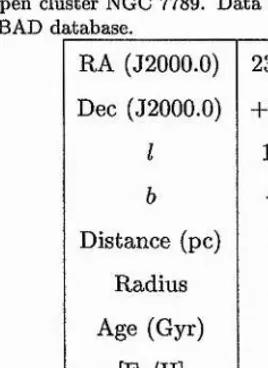
3.1 Properties of the open cluster NGC 7789 ... 57

3.2 Readout noise and gain for each c h ip ... 59

3.3 Magnitude offsets between r u n s ... 73

3.4 Number of stars with lightcurves and colours for each ch ip ... 73

3.5 Magnitude offsets used to calibrate the instrumental m a g n itu d e s... 73

4.1 Number of raw transit candidates and remaining transit candidate lightcurves 81 4.2 Star and lightcurve properties for the transit can d id ates... 86

4.3 Lightcurve and companion properties for the transit candidates... 89

4.4 Lightcurve and companion properties for the transit candidates (continued) 90 4.5 Star, companion and lightcurve properties for INT-7789-TR-3 (star 49512) . 113 5.1 The different subsets of stars used when calculating the number of expected transiting planets and false a la r m s ... 127

(11)

List of Figures

1.1 Mean mass h is to g ra m ... 11

1.2 Period histogram and cumulative distribution fu nction ... 12

1.3 Mean mass and period correlation ... 14

1.4 Orbital eccentricity and period correlation... 15

1.5 Empirical cumulative distribution fu n ctio n s... 17

1.6 Planet frequency against stellar metallicity ... 21

2.1 General configuration of a gravitational le n s ... 32

2.2 Configuration of an extra-solar planetary system at the time of a touching (just grazing) eclip se... 36

2.3 General configuration of an extra-solar planetary system at the start of the transit ingress... 36

2.4 Transit lightcurve morphology as a function of planet ty p e ... 41

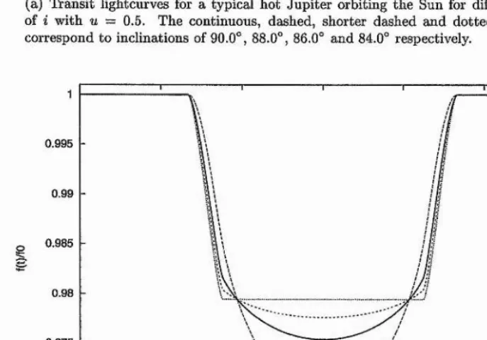
2.5 Transit lightcurve morphology as a function of inclination and the linear limb darkening coefficient... 43

2.6 Typical photometric observations of a transit e v e n t... 46

3.1 Variance versus signal for each ch ip ... 60

3.2 Diagnostic data for Chip 4 ... 61

(12)

LIST OF FIGURES viii

3.4 Instrumental colour magnitude diagrams for each c h i p ... 68

3.5 Instrumental CMD for Chip 4 ... 69

3.6 Plots of Sloan r' magnitude and lightcurve RMS against stellar radius . . . 72

3.7 Mass-radius relationship for the theoretical main sequence... 75

3.8 Theoretical and observed main sequence relations in the Mr versus R — I domain ... 76

4.1 An example boxcar transit f i t ... 80

4.2 Plot of the transit statistic against the out-of-transit reduced chi squared . 82 4.3 Eclipsing binaries with undetermined periods ... 93

4.4 Eclipsing binaries with undetermined p e rio d s ... 94

4.5 Eclipsing binaries with undetermined p e rio d s ... 95

4.6 Eclipsing binaries exhibiting secondary eclip ses... 98

4.7 Eclipsing binaries exhibiting ellipsoidal variations and heating effects . . . . 99

4.8 Possible long period cataclysmic variable... 102

4.9 Stars 6995 and 7628 ... 104

4.10 Stars 22738 and 50313 ... 105

4.11 Stars 64804 and 73852 ... 106

4.12 Planetary transit candidates 45134, 46691 and 49512 ... 110

4.13 Eclipsing binary fits for star 49512 ... I l l 4.14 Finding charts ... 117

5.1 Detection probability and false alarm rate as functions of detection threshold and period for a single s t a r ... 125

5.2 Number of expected transiting planets and false alarms for all stars as func tions of the detection threshold for two different p e rio d s ... 129

(13)

LIST OF FIGURES ix 5.4 Number of expected transiting planets and false alarms for all stars as func

tions of the detection threshold for different planet ty p e s... 133

5.5 Number of expected transiting planets as a function of the detection thresh old for different star types and planet ty p e s ... 134

5.6 The upper limit on the planet fraction as a function of star type and planet t y p e ... 139

A .l General configuration of an extra-solar planet in a circular o rb it... 146

A.2 Definition of the rcy-plane for the extra-solar p la n et... 146

(14)

1 Introduction

1.1 T h e D iscovery O f E xtra-Solar P la n e ts

Some of the first steps towards answering one of humanity’s most fundamental questions about the Universe, “Are we alone?”, lie in the search for planets that orbit stars other than the Sun. Such planets are termed extra-solar planets (or exoplanets). Earth is the only life-bearing planet that we know of and we might expect other solar systems to be similar to our own by assuming that we are not special in any way. Once we know of other planetary systems we may start to look for evidence of life through the detection of biomarkers, chemical elements associated with life processes on Earth, in the spectra of light from an exoplanet. Any speculation on what this life may actually be like lies in the realm of science fiction for the near future.

(15)

1.1 The Discovery O f Extra-Solar Planets 2 dynamics allowed the measurement of the true masses and orbital inclinations of the inner two planets (Wolszczan 1994; Konacki, Maciejewski, & Wolszczan 2000; Konacki & Wol szczan 2003). Pulsars (rapidly rotating neutron stars) are formed during supernovae. The detected planets may have survived a supernova explosion or they may have formed from an accretion disk after the supernova phase. However, both of these evolutionary paths and the hostile pulsar environment imply that these planets are unlikely to harbour life (as we know it!).

The defining breakthrough came in November 1995 with the first detection by Mayor & Queloz (1995) of a Jupiter mass planet orbiting a main sequence star, 51 Pegasi. By measuring the radial velocity of the host star during four different epochs, periodic variations were detected that could be fitted adequately by the presence of a 0.47M j/sin* mass planet orbiting in a 4.23 day circular orbit of radius 0.05AU, where M j is the mass of Jupiter and i is the orbital inclination to the line of sight (* = 90° when the line of sight lies in the plane of the orbit). It is impossible to determine the value of sin* by use of the radial velocity technique alone, and therefore the mass derived for the planetary companion serves as a lower limit. Having said this, assuming that no particular orbital inclination is preferred, then with greater than 99% probability the mass of the companion is < 3.5Mj (see Appendix A, Example 1). By considering constraints originating from the observed rotational velocity of 51 Pegasi (Soderblom 1983; Baranne, Mayor, & Poncet 1979) and its low chromospheric emission (Noyes et al. 1984), Mayor & Queloz (1995) were able to give an upper limit of 2M j for the mass of the companion.

(16)

1.1 The Discovery O f Extra-Solar Planets 3 Meanwhile Marcy et al. (1997) published more radial velocity measurements showing the 4.23 day periodicity and stating that the only viable interpretation was one of a Jupiter mass companion. However, a general consensus was reached that the radial velocity variations were most consistent with a planetary companion with the publication by Hatzes, Cochran, &: Bakker (1998) of a lack of spectral variability in 51 Pegasi, refuting their own previous claims.

Soon after the discovery of 51 Pegasi b (the letter b denotes the reference to the planet rather than the star), other groups announced more planet candidates from radial velocity (RV) surveys (Butler & Marcy 1996; Marcy & Butler 1996; Butler et al. 1997) leading to an explosion in the number of planetary detections. With an ever increasing time baseline for the RV measurements, it has been possible to detect planets of longer periods, conse quently probing larger orbital distances from the host stars. The Mp sin* detection limit is determined by the precision of the RV measurements which typically ranges from ~10ms~^ for the smaller telescopes (Baranne et al. 1996) to ~3ms“ ^ for the larger telescopes (Tinney et al. 2001). Improvements in the efficiency of the spectrographs employed in the detection of extra-solar planets has increased the precision obtained from the RV measurements to around '^l-2ms~^ (Pepe et al. 2004). However, there seems to be a fundamental limit to the attainable precision defined by the intrinsic velocity stability of the target stars (Saar, Butler, & Marcy 1998; Saar & Fischer 2000). Such RV variations, commonly called “jit ter”, are induced by the rotation of star spots and/or convective inhomogeneities and their temporal evolution. It should also be noted that the RV technique is limited to surveying bright target stars in order to provide the necessary high signal to noise (S/N) spectra. As a consequence, this limits the RV surveys to Solar neighbourhood stars. There has also been a tendency to target main sequence stars similar to our Sun in the quest to find a Solar System analogue. For instance, the Anglo-Australian planet search targets F, G and K main sequence stars down to V=7.5 mag (Jones 2002).

(17)

1.2 Characteristics O f The Extra-Solar Planets 4 http://www.obspm.fr/encycl/catl.html

1.2 C haracteristics O f T h e E xtra-Solar P la n e ts

At this stage, clarification is required as to exactly what class of objects are defined to be

planets. An object with a mass greater than ^O.OSMq =84Mj has a core temperature high

enough to ignite the thermonuclear fusion of hydrogen, and hence to self luminesce. This object is a star and stars are thought to form from the collapse of rotating interstellar gas and dust clouds via gravitational instability (Boss 1980). The minimum mass required to form an object via the gravitational collapse of such a gas cloud is thought to lie in the range 7-20Mj (Boss 1986). Objects formed this way with a mass less than ~O.O8M0 are referred to as brown dwarfs (Tarter 1986; Burrows & Liebert 1993). They emit radiation mainly in the infrared owing to the thermal energy of their creation and for brown dwarfs with masses greater than ~12M j, deuterium fusion in their cores will contribute to their luminescence.

Planets are thought to form via the agglomeration and accretion of material within the gas and dust disk of a protostax, and planets do not luminesce via thermonuclear fusion at any stage during their lifetimes. The lower mass limit of ~12M j for deuterium fusion depends weakly on various factors (chemical composition etc.) and therefore a safe upper mass limit for planets of ~10M j will be adopted here. It must be pointed out that since brown dwarfs may also form as stellar companions, there lies a “grey” area between what constitutes a planet and what constitutes a brown dwarf.

(18)

1.2 Characteristics O f The Extra-Solar Planets

(19)

1.2 Characteristics O f The Extra-Solar Planets

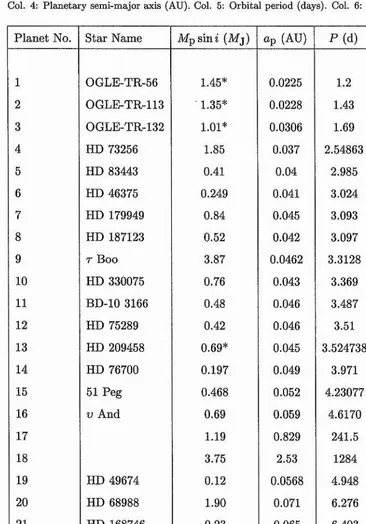
Table 1.1; Extra-solar planet catalogue ordered by increasing period of innermost planetary companion. Col. 4: Planetary semi-major axis (AU). Col. 5: Orbital period (days). Col. 6: Orbital eccentricity.

Planet No. Star Name Mp sin* (M j) Op (AU) P (d ) e

1 OGLE-TR-56 1.45* 0.0225 1.2 0.0

2 OGLE-TR-113 ■ 1.35* 0.0228 1.43 0.0

3 OGLE-TR-132 1.01* 0.0306 1.69 0.0

4 HD 73256 1.85 0.037 2.54863 0.038

5 HD 83443 0.41 0.04 2.985 0.08

6 HD 46375 0.249 0.041 3.024 0.04

7 HD 179949 0.84 0.045 3.093 0.05

8 HD 187123 0.52 0.042 3.097 0.03

9 T Boo 3.87 0.0462 3.3128 0.018

10 HD 330075 0.76 0.043 3.369 0.0

11 BD-10 3166 0.48 0.046 3.487 0.0

12 HD 75289 0.42 0.046 3.51 0.054

13 HD 209458 0.69* 0.045 3.524738 0.0

14 HD 76700 0.197 0.049 3.971 0.0

15 51 Peg 0.468 0.052 4.23077 0.0

16 V And 0.69 0.059 4.6170 0.012

17 1.19 0.829 241.5 0.28

18 3.75 2.53 1284 0.27

19 HD 49674 0.12 0.0568 4.948 0.0

20 HD 68988 1.90 0.071 6.276 0.14

21 HD 168746 0.23 0.065 6.403 0.081

22 HD 217107 1.28 0.07 7.11 0.14

23 HD 130322 1.08 0.088 10.724 0.048

[image:19.613.68.434.145.669.2]

(20)

1.2 Characteristics O f The Extra-Solar Planets continued from previous page

Planet No. Star Name Mp sin* (Mj) dp (AU) f (d) e

24 HD 108147 0.41 0.104 10.901 0.498

25 HD 38529 0.78 0.129 14.309 0.29

26 55 Cnc 0.84 0.11 14.65 0.02

27 4.05 5.9 5360 0.16

28 G1 86 4.0 0.11 15.78 0.046

29 HD 195019 3.43 0.14 18.3 0.05

30 HD 6434 0.48 0.15 22.09 0.30

31 HD 192263 0.72 0.15 24.348 0.0

32 Gliese 876 0.56 0.13 30.1 0.12

33 1.98 0.21 61.02 0.27

34 pCr B 1.04 0.22 39.846 0.04

35 HD 74156 1.86 0.294 51.643 0.636

36 HD 37605 2.85 0.26 55.2 0.736

37 HD 168443 7.7 0.29 58.116 0.529

38 HD 3651 0.2 0.284 62.23 0.63

39 HD 121504 0.89 0.32 64.6 0.13

40 HD 178911 B 6.292 0.32 71.487 0.1243

41 HD 16141 0.23 0.35 75.560 0.28

42 HD 80606 3.41 0.439 111.78 0.927

43 70 Vir 7.44 0.48 116.689 0.4

44 HD 216770 0.65 0.46 118.45 0.37

45 HD 52265 1.13 0.49 118,96 0.29

46 GJ 3021 3.21 0.49 133.82 0.505

47 HD 37124 0.75 0.54 152.4 0.10

48 1.2 2.5 1495 0.69

49 HD 219449 2.9 0.3 182 0.0

(21)

Planet No. Star Name M p sin * (Mj) Op (AU) f (d) e

50 HD 73526 3.0 0.66 190.5 0.34

51 HD 104985 6.3 0.78 198.2 0.03

52 HD 82943 0.88 0.73 221.6 0.54

53 1.63 1.16 444.6 0.41

54 HD 169830 2.88 0.81 225.62 0.31

55 4.04 3.60 2102 0.33

56 HD 8574 2.23 0.76 228.8 0.40

57 HD 89744 7.99 0.89 256.6 0.67

68 HD 134987 1.58 0.78 260 0.25

59 HD 12661 2.30 0.83 263.6 0.096

60 1.57 2.56 1444.5 0.1

61 HD 150706 1.0 0.82 264.9 0.38

62 HD 40979 3.32 0.811 267.2 0.25

63 HD 59686 6.5 0.8 303 0.0

64 HD 810 2.26 0.925 320.1 0.161

65 HD 142 1.36 0.980 338.0 0.37

66 HD 92788 3.8 0.94 340 0.36

67 HD 28185 5.6 1.0 385 0.06

68 HD 142415 1.62 1.05 386.3 0.5

69 HD 177830 1.28 1.00 391 0.43

70 HD 4203 1.65 1.09 400.944 0.46

71 HD 108874 1.65 1.07 401 0.20

72 HD 128311 2.63 1.06 414 0.21

73 HD 27442 1.28 1.18 423.841 0.07

74 HD 210277 1.28 1.097 437 0.45

75 HD 19994 2.0 1.3 454 0.2

(22)

Planet No. Star Name Mp sin* (Mj) (Zp (AU) f (d) e

76 HD 20367 1.07 1.25 500 0.23

77 HD 114783 0.9 1.20 501.0 0.1

78 HD 147513 1.0 1.26 540.4 0.52

79 HIP 75458 8.64 1.34 550.651 0.71

80 HD 222582 5.11 1.35 572.0 0.76

81 HD 65216 1.21 1.37 613.1 0.41

82 HD 160691 1.7 1.5 638 0.31

83 HD 141937 9.7 1.52 653.22 0.41

84 HD 41004A 2.3 1.31 655 0.39

85 HD 47536 4,96 1.61 712.13 0.20

86 HD 23079 2.61 1.65 738.459 0.10

87 16 Cyg B 1.69 1.67 798.938 0.67

88 HD 4208 0.80 1.67 812.197 0.05

89 HD 114386 0.99 1.62 872 0.28

90 7 Cephei 1.59 2.03 902.96 0.2

91 HD 213240 4.5 2.03 951 0.45

92 HD 10647 0.91 2.10 1040 0.18

93 HD 10697 6.12 2.13 1077.906 0.11

94 47 Uma 2.41 2.10 1095 0.096

95 0.76 3.73 2594 0.1

96 HD 190228 4.99 2.31 1127 0.43

97 HD 114729 0.82 2.08 1131.478 0.31

98 HD 111232 6.8 1.97 1143 0.20

99 HD 2039 4.85 2.19 1192.582 0.68

100 HD 50554 4.9 2.38 1279.0 0.42

101 HD 196050 3.0 2.5 1289 0.28

(23)

1.2 Characteristics O f The Extra-Solar Planets 10

continued from previous page

Planet No. Star Name Mpsin* (Mj) Up (AU) f (d) e

102 HD 216437 2.1 2.7 1294 0.34

103 HD 216435 1.49 2.7 1442.919 0.34

104 HD 106252 6.81 2.61 1500 0.54

105 HD 23596 7.19 2.72 1558 0.314

106 14 Her 4.74 2.80 1796.4 0.338

107 HD 72659 2.55 3.24 2185 0.18

108 HD 70642 2.0 3.3 2231 0.1

109 HD 33636 9.28 3.56 2447.292 0.53

110 € Bridani 0.86 3.3 2502.1 0.608

111 HD 30177 9.17 3.86 2819.654 0.30

112 G1 777A 1.33 4.8 2902 0.48

(24)

20

15

I 10 0)

6 8 10

Mean Mass (Jupiter Masses)

12 14 16

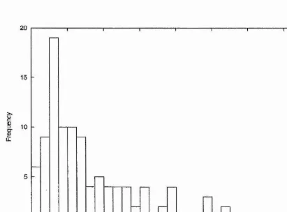
Figure 1.1: Histogram of the mean mass of the extra-solar planets.

1.2.1 The M ass And Period D istributions

Radial velocity measurements of a planet host star supply the observable quantity Mp sin i

as a lower limit to the mass of the extra-solar planet (see Section 2.1). Making the as sumption that the orbital orientation of the extra-solar planet is random means that we can calculate the mean mass (Mp) of the extra-solar planet as (Mp) = ^Mp sin* (see Ap pendix A, Example 2). Figure 1.1 shows a histogram of the mean mass distribution for the extra-solar planets listed in Table 1.1. The mean mass distribution rises towards lower masses down to ~ lM j. The failure to rise any further for even lower masses is due the limited detectability of these planets using the RV technique.

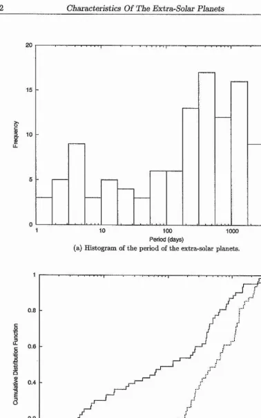
[image:24.614.71.482.120.424.2]

(25)

20

15

I "

10 100 1000

Period (days)

(a) Histogram of the period of the extra-solar planets.

10000

0.8

I

c 0.6 .9

I

Ê

0.4

I

Ü 0.2

1 10 100 1000 10000

Period (days)

(b) Cumulative distribution function against period for the less massive extra-solar plan ets ((Mp) < 3Mj with the continuous line) and for the more massive extra-solar planets ((Mp) > 3Mj with the dashed line).

[image:25.612.85.464.89.694.2]

(26)

1.2 Characteristics O f The Extra-Solar Planets 13 The period distribution shows a sharp cut off at around ~3 days, especially if we ignore the 3 recently discovered OGLE planets that seem to form part of a new class of planets (“very hot Jupiters”). The period distribution then drops towards higher periods and rises abruptly again for periods ;^100 days, revealing a “period valley” for periods between ~10 and ~100 days (Udry, Mayor, & Santos 2003). Observationally, this may be explained by the combination of two different planet populations, a lower mass planet population that peaks at short periods and extends to longer periods, and a higher mass planet population that almost exclusively has periods j^lOO days. The existence of the two populations is illustrated clearly in Figure 1.2(b) where we plot the cumulative distribution function (CDF) against period for two planet populations, the less massive extra-solar planets ((Mp) < 3M j with the continuous line) and the more massive extra-solar planets ((Mp) > 3Mj with the dashed line). The statistical significance of the lack of higher mass planets on short periods has been verified by Zucker & Mazeh (2002) and Udry, Mayor, & Santos (2003) using the fact that if such planets existed then they should be easily detectable by the RV technique.

Figure 1.3 shows a scatter plot of the mean mass against period for the extra-solar planets. The rectangular region in the upper left of the diagram delimited by the dashed line highlights the region with few higher mass planets at short periods ((Mp) > 3M j and

(27)

I

100

Period (days)

10000

Figure 1.3: Plot of mean mass against period for the extra-solar planets. Filled circles represent planets that orbit in single-star systems. Circles with dots represent planets that orbit in multiple-star systems.

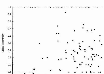
1.2.2 The Orbital Eccentricity And Period Correlation

The extra-solar planets with the smallest orbital semi-major axes (shortest periods) are likely to have undergone orbital circularisation via tidal interaction with the host star. A scatter plot of orbital eccentricity against period (Figure 1.4) clearly shows that all extra solar planets with periods of less than 6.0 days have orbital eccentricities of less than 0.1 (lower left rectangular region delimited by a dashed line) indicative of circular orbits. Removing these planets from our sample and calculating the Spearman’s rank correlation coefficient between orbital eccentricity e and period F yields rgs = 0.2277... % 0.228. Assuming a null-hypothesis that e and P are uncorrelated allows one to calculate, for a given N , the probability of obtaining a value of greater than or equal to k where

[image:27.614.72.484.140.422.2]

(28)

0.9

0.8

0.7

i

0.6

0.3

0.2

0.1

0 • i ;

• • •

• • • # 0

• • • • •

• • •

#

# • # # *

* *

#

# # • • ! • • •

10 100

Period (days)

1000 10000

Figure 1.4: Plot of orbital eccentricity against period for the extra-solar planets.

the test and the smaller the value of P(|riv| > k), the less likely we are to reject the null- hypothesis when it is actually correct (Type I error). If we choose a significance level a

[image:28.613.72.483.133.424.2]

(29)

1.2.3 H o t J u p ite rs A nd T h eir P ro p e rtie s

The discovery of close-in Jupiter-mass companions to main sequence stars was not antici pated by the pre-discovery theories of planetary formation (see Section 1.3). Such planets were termed “hot Jupiters” due to the expected heating of the planets by the host stars and they were found to have a period cut off at the low end of the period distribution of ~3 days. It was only very recently that planets with a period of less than ~3 days were discovered: OGLE-TR-56b (Konacki et al. 2003b), 0GLE-TR-113b and OGLE-TR-132b (Bouchy et al. 2004). Such planets have been termed “very hot Jupiters”.

In this section, we will consider the subsample of extra-solar planets termed “hot Jupiters” defined by P < 10.0 days and excluding the “very hot Jupiters”. The upper limit to the period is chosen to coincide with the start of the “period valley” discussed in Section 1.2.1 but otherwise it is arbitrary. We will try to derive the simplest continuous underlying PDFs for the period P , orbital semi-major axis Up, eccentricity e and mean mass (Mp). We will use these analytic representations of the hot Jupiter distribution functions in Chapter 5 when doing Monte Carlo simulations. The analysis below follows the method of Heacox (1999).

Let us define the empirical cumulative distribution function (ECDF) for ordered data

< ^ 2 < ■ ■ ‘ < X M h y :

P M =

- for (1.1)

We have fitted a continuous function G(x) to each ECDF by iterating a weighted least

squares fit with weights (Stuart & Ord 1987) defined by:

2 _ G(xj)(l - G(xj))

Figure 1.5 shows plots of F ( x j ) against Xj for each of P , &p, e and (Mp). Each plot in Figure 1.5 shows the specific function fitted to the ECDF as a continuous line and the ± lc r

curves as dashed lines. The results of the fits are shown in Table 1.2.

(30)

(a) Plot of F(P) against P for the hot Jupiters along with the fitted function G(P).

0.8

(b) Plot of P(ttp) against ap for the hot Jupiters along with the fitted function G(ap).

0.1 OtbHai Eccentricity

(c) Plot of P(e) against e for the hot Jupiters along with the fitted function G(e).

0.1

Mean M ass (Jupiter Masses)

[image:30.613.71.506.159.574.2]

(d) Plot of F((Mp}) against (Mp) for the hot Jupiters along with the fitted function G((Mp}).

(31)

Table 1.2: Results of the fits of G(æ) to F(x) including the K-S statistic (Col. 7) and its significance (Col. 8).

X Units Of X G(%) u V CFy k = D u > A)

p d u + v log(æ) -0.734 0.088 2.04 0.13 0.178 0.608 AU u + v log(rc) 0.23 3.18 0.18 0.176 0.626

e - u + v^/x 0.112 0.027 2.32 0.12 0.211 0.389

(32)

(Heacox 1999) since we have individual data points (not grouped data). The K-S statistic

D]v is defined by:

D]sr — max \G{xj) — F{xj)\ (1.3)

Assuming a null-hypothesis that Xj is drawn from the underlying CDF G{x) allows one to

calculate, for a given AT, the probability of obtaining a value of greater than or equal to

k where A; 6 M. This probability is denoted hy P{Djsf > k). Table 1.2 reports the values of

k = D u obtained for the fits along with the probabilities P(Djv > k) for N ~ 17. One can see from Table 1.2 that we cannot reject the null-hypothesis at the a = 0.05 significance level for any of the fits. Hence, for any of P, Op, e and (Mp), we do not need to hypothesise a closer fit to the data. Summarising the results, we have GDPs of the form:

G{P) = u P vlog{P) G{ap) = ■a + ^;log(ap)

G{e) = u p vy/e

G((Mp)) = u P v log((Mp))

(1.4)

The corresponding PDFs are found by differentiating:

g(P) oc P-^

g{ap) oc a~^ g{e) oc e~^-^ g{{Mp)) oc (M p)~^

1.2.4 Planet Frequency And Stellar M etallicity

(1.5)

(33)

decide which model is most likely to be correct. As humans, we also want to know if the factors that are responsible for our origin and existence have selected a non-typical location.

The data that we have on extra-solar planets has already shown that Jupiter is a typical giant planet in the sense that it lies in the most densely occupied region of the log(Mp) — log(P) plane (Lineweaver & Grether 2002; Lineweaver, Grether, & Hidas 2003). Analysis of the <^1800 Sun-like stars that were being monitored by RV surveys at the end of 2003 has revealed the following facts (Lineweaver & Grether 2003);

1. At least ~5% of target stars possess at least one planet.

2. Limiting the sample to target stars that have been monitored for ;^15 years indicates that at least ~ 11% possess at least one planet.

3. Limiting the sample to target stars that have been monitored for ;^15 years and whose low surface activity allows the most precise RV measurements indicates that at least ^25% possess at least one planet.

It is clear that the longer we survey stars with the RV technique, and the better the accuracy that we achieve, the greater the fraction of stars found to harbour at least one planet. For the work in this thesis, the most pertinent question is “W hat fraction of main sequence stars have hot Jupiters, and how does this depend on the host star properties?”. Butler et al. (200,0) provide an estimate that ~1% of nearby Sun-like stars (late F and G dwarfs) host a hot Jupiter (3.0 < P < 5.0 days).

Recently it has come to light that stars with planets seem to be particularly metal rich when compared with “single” (non-binary and no planet found to date) field dwarfs (Santos et al. 2003; Santos, Israelian, & Mayor 2004). The metallicity of a star, denoted by [Fe/H] and with units dex, is defined relative to the Solar metallicity by:

[Fe/H] = logCArpe/WH). - lo g ( # e /% ) o (1.6)

(34)

§ 20

^ 0.2

j

B

■0.5

0

[Pe/H3

Figure 1.6: Taken from Santos, Israelian, & Mayor (2004). Left: Normalised histogram of the stellar metallicities for planet host stars (shaded) and for “single” stars (clear). Right: The percentage of stars with planets against stellar metallicity.

star subsamples taken from the volume limited CORALIE star sample (Udry et al. 2000).

The shaded histogram represents the metallicity distribution of the 48 stars with known planets, and the clear histogram represents the metallicity distribution of 875 non-binary stars with no planet found to date. One can clearly see the trend to higher metallicities for stars with planets compared to those stars without. Although some authors have claimed that the source of the metallicity excess for planet host stars lies in the process of planetary formation via accretion of disk material and/or planets themselves (Gonzalez 1998), the strongest evidence points to a primordial origin (Sadakane et al. 2002; Santos et al. 2003).

(35)

1.3 Star And Planetary Formation 22

found.

1.2.5 The Variety O f Extra-Solar Planets

At this point it would be appropriate to highlight the variety of extra-solar planetary systems detected to date with a couple of examples. We have already met the hot Jupiters (and very hot Jupiters), and also the pulsar planets, both of whose discovery surprised the astronomical community. It is interesting to note that we know of 8 multiple planetary systems to date (see Table 1.1). In particular the star v Andromedae has a triple planetary system, and it was the first reported multiple planetary system around a main sequence star (Butler et al. 1999). The system consists of a hot Jupiter and two planets more massive than Jupiter in eccentric orbits with semi-major axes 0.83AU and 2.5AU. This is obviously not a Solar System analogue, but it illustrates the possibility that stars with a single extra solar planet may have other planetary companions with periods too long or masses too small to have been detected yet. Planetary systems are not limited to single stars either. The stellar system of 16 Cygni is actually a triple star system composed of a wide visual binary of two G dwarfs and a distant M dwarf. The G2.5V star 16 Cygni B has a Jupiter mass planetary companion in a very eccentric orbit of semi-major axis 1.7AU (Cochran et al. 1997). Such a variety of planetary systems (in which we must include our own) challenges our theories planetary formation and helps to constrain the likely formation scenarios. Thus it is imperative to keep expanding our database of known extra-solar planets over a range of stellar types and environments.

1.3 Star A nd P la n eta ry F orm ation

1.3.1 Star Formation

(36)

1.3_____________________Star And Planetary Formation _________________ 23 The details of the collapse, including the effects of stellar rotation and magnetic fields, are complex and incompletely known, but they may be roughly split into two stages.

The first stage is characterised by free-fall collapse due to the fact that the inner parts of the cloud contract under self-gravity faster than the outer parts of the cloud. The free-fall time for a test particle of mass m at the edge of a uniformly collapsing spherical cloud of mass M , radius R and initial density po may be calculated by considering that it will follow an orbit of semi-major axis a = R/2, period P and eccentricity e = 1. Substituting the expression for the density of the cloud:

M = (1.7)

into Kepler’s third law:

and using the fact that a = R /2 gives:

The free-fall time tg is half of the period P and hence for a cloud of typical density 10“ ^^kg/m^ the time scale for initial collapse is tQ ~ 10® years.

Interstellar clouds rotate at least a bit, and an isolated rotating cloud must conserve angular momentum. Hence, as the cloud collapses and each particle moves closer to the axis of rotation, the cloud starts to rotate faster. At some point for each particle, the angular speed will become high enough that the centripetal acceleration balances the gravitational force and the particle stops moving closer to the axis of rotation. However, each particle will continue moving parallel to the axis of rotation and as a result, most of the infalling material misses the protostar and ends up in the equatorial plane. This leads to the formation of a disk structure from the initial “spherical” configuration of the interstellar cloud.

(37)

the geometry of the disk, causes bipolar outflows of gas which carry away ^ 10"®—

per year. This mass loss from the system also carries away angular momentum that brakes the rotation of the protostar in ~10® years.

1.3.2 Planet Formation

Planet formation is thought to follow on from the process of star formation via the agglom eration of material within the circumstellar (protoplanetary) disk (Perryman 2000; Ida & Lin 2004). A dust layer starts to form near the central plane of the disk via the sedimenta tion of dust grains. When the density of the dust layer exceeds some critical value, the dust grains start to stick together as they collide, forming conglomerations called planetesimals. The planetesimals also start colliding with one another, the majority of the collisions being non-destructive, so that the planetesimals start to grow in size. The larger a planetesimal the faster it grows leading to runaway growth. The largest planetesimals sweep up all other planetesimals with orbital semi-major axes similar to their own to become the first proto planets. The regions near the protoplanets are continuously supplied with planetesimals from the rest of the disk by orbital migration due to gravitational scattering and viscous drag from the disk gas. When a protoplanet reaches a mass of ^lOM© (where M© is the mass of the Earth), it will start to accrete gas in addition to planetesimals. As this process of planet formation is continuing, the gas and dust of the disk is being blown gradually out of the system by the stellar wind emanating from the protostar until eventually there is very little left to be accreted by the protoplanets. W ith the supply of planetesimals running out as well, the growth of the protoplanets finally ceases. Table 1.3 shows the approximate timescales and particle/object sizes for each of the stages described above. It should be noted that the timescales shown vary significantly with orbital radius and that the exact details of the formation theory are poorly understood, and so these values should be treated with caution.

(38)

Table 1.3: Approximate duration and typical particle/object sizes for each of the stages in the core accretion model of planetary formation (Zeilik fc Gregory 1998; Perryman 2000).

Stage Typical Duration Typical Particle Size/Mass

Sedimentation of dust grains Formation of planetesimals Formation of protoplanets Formation of planets

10^—10® years 10“^—10® years 10® —10® years 10^—10® years

0.01/im—lyum Im —1km

10“®M©-10-^M©

(39)

1.3 Stax And Planetary Formation 26 1. The temperature close to the protostar is too high for gas (and ice) accretion to take

place.

2. The gas is blown away first from the inner parts of the protostellar disk.

3. The total mass of the disk material closer in to the protostar is smaller.

As one can see, the core accretion model alone is not sufficient to account for the existence of hot Jupiters. To deal with this, it has become common to invoke orbital migration.

1.3.3 Planet M igration

The possibility of planetary migration was actually suggested before the discovery of hot Jupiters (Goldreich & Tremaine 1980). A protoplanet may undergo rapid Type I orbital migration towards the star if it is not yet massive enough to open and sustain a gap in the disk. The migration occurs as a result of torque asymmetries due to the gravitational interaction of the protoplanet with the disk. If the orbital decay time is shorter than the life of the disk, then the protoplanet is in danger of being accreted into the star. At /-^lAU the migration timescale for a ~1M© protoplanet is only 10"^—10® years (Ward 1997) compared to a disk lifetime of ~10^ years (Nakano 1987). Also, Type I migration seems inconsistent with the prolific formation of giant extra-solar planets since the protoplanetary cores have a tendency to rapidly migrate to the proximity of their host stars prior to gas accretion.

If gap formation in the disk is successful due to a massive enough protoplanet, then Type II migration will occur. In this case the protoplanet has effectively established a barrier to any radial flow of disk material due to viscous diffusion and the protoplanet becomes locked into the disk (Lin &: Papaloizou 1986). Orbital migration is in either direction, and although slower than Type I migration, it may still put a protoplanet in danger of destruction under the right conditions.

(40)

1.4 Summary 27

any protoplanet that migrates to very close distances to the host star (^O.OSAU) is most likely to be accreted and we would not observe such an abundance of hot Jupiters. Several potential mechanisms have been put forwards as to how an inwardly migrating planet may be halted at small orbital radii (Lin, Bodenheimer, & Richardson 1996; Trilling et al. 1998). These include the hypothetical existence of a low-density zone maintained by magnetic coupling to the disk, tidal interaction with the spinning star and mass transfer from the protoplanet to the star.

1.4 Sum m ary

(41)

2

A Mena

gerie Of Detection Techniques

Up to now, almost all of the extra-solar planet detections have been made by the radial velocity technique despite a number of alternative viable methods being pursued vigorously. This chapter deals with the question “W hat techniques are being brought to bear on the problem of extra-solar planet detection and what results may we reasonably expect from them?”.

(42)

2.1 Radial Velocity 29

see Appendix B.

— Luminosity of the star/planet. M*,Mp — Mass of the star/planet.

iî*,iîp — Radius of the star/planet

n*,ap — Semi-major axis of the orbit of the star/planet about the centre of mass.

P — Orbital period of the planet, e — Orbital eccentricity.

i — Orbital inclination, w — Longitude of periastron.

2.1 R ad ial V elocity

An extra-solar planet and its host star orbit their common centre of mass, and hence the star undergoes periodic variations in its velocity along the line of sight (radial velocity). The semi-amplitude K of this variation (see Appendix C, Theorem 3) is given by:

f ; (M* Mp)2/3(1 - e2)i/2

For a circular orbit (e — 0) and for Mp M*, the semi-amplitude reduces to:

(43)

2.2 Direct Imaging And ReÛected Light 30

A radial velocity measurement of a star is made by obtaining a high signal to noise spectrum using a high resolution spectrograph with typically an I2 gas absorption cell. The I2 cell provides a wealth of absorption lines superimposed on the stellar spectral lines. This facilitates the measurement of the Doppler shift AA of the light of wavelength A arriving from the star relative to the Earth, yielding the star’s radial velocity Vr = cAA/A. Using an accurate ephemeris to correct for the Earth’s motion, a set of radial velocity measurements well sampled in time will yield the heliocentric radial velocity curve for the star. The curve may be fitted by the model in Appendix C (Theorem 2), yielding values for P , e, u and Mp $in%/(M* 4- Mp)^/®. The value of M* may be estimated from the spectral type of the star under observation, and using the approximation M* + Mp « M$ for Mp -C M*, one may estimate M psini, a lower limit for the value of Mp. To obtain a value of the mean star-exoplanet distance n = a* 4- ap % Up, one may use Kepler’s third law (Equation 1.8 with M = M* 4- Mp % M*).

The radial velocity technique has been used to discover almost all confirmed extra-solar planets to date making it the most important method so far in the hunt for these objects. In Sections 1.1 and 1.2.5 we have mentioned the relevant references to RV surveys and their discoveries. We have also already noted the Mpsin? ambiguity (Appendix A), the intrinsic limit to the precision of RV measurements due to “jitter”and the limitation of a RV survey to the Solar neighbourhood (Section 1.1).

2.2 D ire c t Im a g in g A n d R e fle c te d L ig h t

(44)

2.2__________________Direct Imaging And Rejected Light___________________ ^

we may calculate the luminosity of the extra-solar planet Lp via reflected light as:

L p = p ( A , a ) l 0 l £ . (2.3)

At a distance of lOpc from our Solar System, Jupiter and the Sun have an angular separation of ~0.52" at maximum elongation. In this configuration we would observe half of the planetary disk as illuminated (a half-Jupiter), which leads us to set p(A, a) % 0.5 in the best case scenario. Hence Equation 2.3 yields a contrast of Lp/L* % 2.1 x 10~^. From the ground, the planetary signal is immersed in the photon noise of the telescope’s diffraction profile and the star’s seeing profile (typical seeing 0.5" - 1.0") making it undetectable.

Efforts are under way to minimise these problems by employing the following techniques:

1. Suppressing scattered light using a coronograph.

2. Reduction of the angular size of the star profile using adaptive optics.

3. Observing in the infrared where the value of Ap/L* is around 10® times larger (due to thermal emission from the planet itself).

4. Using interferometric nulling to cancel out the light from the star.

5. Observing from space to eliminate the effects of atmospheric turbulence.

Although the direct imaging method has not been successfully applied to extra-solar planet detection so far, it will in the future be capable of providing broadband colours, spec tral features and spectral energy distributions, giving constraints on the temperature and chemical composition of the planet atmosphere/surface, including revealing the presence of biomarkers (O3, O2, H2O etc.). This makes direct imaging the technique which has the potential to produce results with the biggest scientific impact.

(45)

2.3 Gravitational Microlensing 32

\ Ij0^5 PU»\e.

Figure 2.1: General configuration of a gravitational lens.

high resolution spectra and, by carefully modelling and removing the star’s spectrum, the reflected light spectrum will be left. A total of three extra-solar planetary systems have been observed in this way (Cameron et al. 2002; Leigh et al. 2003a; Leigh et al. 2003b). Although the reflected spectra were not detected unambiguously, the technique was used to place limits on the geometric albedo p of each extra-solar planet {p < 0.22 for v And b,

p < 0.39 for r Boo b and p < 0.12 for HD 75289b).

2.3 G ravitation al M icrolensin g

Gravitational lensing is the focusing of light rays from a distant source by an intervening ^ massive object (called the lens). The focusing of the light rays produces a magnification of the brightness of the source object. Figure 2.1 shows the configuration of a typical gravitational lens in which the observer sees two images of the source object. If the source lies directly behind the lens as viewed by the observer, then the source forms an image ring at a radius called the “Einstein radius” of the lens.

(46)

(Wambsganss 1997) is given by:

■Re =

1/2

(2.4) 4 G M l(£ > s -J > l)P l

. c" Ds .

where M l is the mass of the lens object and the distances Dg and £>l are as defined in

Figure 2.1. The Einstein angle % is expressed in angular units:

^ (2-5)

Looking at source stars in the Galactic bulge (Dg % 8kpc) and considering lens stars at a distance D l ^ 4kpc with approximately solar masses (M l ~ 1M@) yields % 0.001". The angular separation of the two source images is approximately 2 pe 0.002" which is clearly unresolvable by even the best adaptive optics from the ground (resolution ~0.1").

As the source, lens and observer are all in motion, the source will appear to move relative to the lens as viewed by the observer, and the source will undergo a characteristic increase and then decrease in brightness. This is the only observable signature of a microlens, but it is distinguishable from peculiar intrinsic source variability by its achromatic nature. The microlensing magnification A{t) of the source as a function of time t is given by:

" « ( t ) ( t ! ( ] )2 + 4)1/2 (2-®)

where u{t) is the projected distance between the lens and the source in the lens plane in units of as a function of time t. Precise alignment of the lens and source is required for a detectable source brightening and hence the probability of substantial microlensing magnification is extremely small 10“ ® for source stars in the Galactic bulge). Timescales for a typical Galactic bulge microlensing event range from days to months (Wambsganss 1997).

(47)

W ith the advent of observational programmes monitoring millions of stars (OGLE: Udalski et al. 1993; MACHO: Alcock et al. 1993 etc.), hundreds of photometric microlens ing events have now been observed. A small subset of the already rare microlensing events have revealed anomalies which are due to a number of different scenarios including binary lenses (Udalski et al. 1994) and the effect of the Earth’s motion around the Sun (Alcock et al. 1995). It is only recently that the first unambiguous planetary microlensing event has been detected (Bond et al. 2004) from the perturbation of the simple lightcurve of an isolated point lens.

(48)

2.4 Transit Photometry 35

2.4 Transit Photometry

Given a fortuitous geometric alignment, an extra-solar planet may be observed to eclipse the host star as viewed from the Earth. Such an eclipse is called a planetary transit and it is characterised by a small decrease in the observed brightness of the host star that repeats at the orbital period of the extra-solar planet.

2.4.1 Transit Probability

Consider an extra-solar planet P of radius Rp orbiting a star S of radius jR* in a circular orbit of radius a. Let i be the orbital inclination of the planet (the angle between the line of sight and the normal to the orbital plane). Figure 2.2 shows the configuration of S and P when the disk of P just touches the disk of S at the “top” of its orbit as projected in the sky plane. It is clear from Figure 2.2 that in order for a transit to occur, the disk of P must obscure the disk of S to some extent. This condition may be written as:

X = asin(90° - i) < 4- JRp (2.7)

Hence the probability P^^^a of observing a transit is given by:

Ptra ~ P(ûsin(90° — î) < iî* -|- iîp)

= (2.8)

Under the assumption that the orbital inclination of the extra-solar planet P is random, we can apply Equation [6] in Appendix A to Equation 2.8, which yields:

7^* + -Rp

tra (2.9)

(49)

Vuaw olUm

g t u . Uvz. ÿ s y ^ t I

Sfe^PW

OcLJbxA

Figure 2.2: Configuration of an extra-solar planet and the host star when the disk of the planet is observed to touch the disk of the star at the “top” of its orbit as projected in the sky plane.

Viu^/ o W tU , Vü2w c i ^ tU . U u l

dcosOsir\(lO-t)

N

(50)

lies fully infront of the disk of the host star at some point during the eclipse. Following similar arguments to those used above, it may be shown that the probability of an annular eclipse Pann of S by P is given by:

ann P (2.10)

Since an eclipse is either annular or grazing we have:

Ptra = P ann + P gra (2.11)

where Pgra is the probability of a grazing eclipse of S by P. Rearranging Equation 2.11 and using Equations 2.9 and 2.10 yields;

o p

Pgra — (2.12)

It is clear from Equation 2.9 that the closer a planet is to the host star, the more likely it is to be observed to transit the stellar disk as seen from the Earth. In fact, for a star of a particular radius, Ptra is maximised for a hot Jupiter. For example, consider a typical hot Jupiter (a % 0.05AU and Rp % 1.4Rj - see Section 2.4.5) orbiting a Sun like star (R* % 1R@). Then we calculate Ptra ^ 0.106. The strongest transit signal occurs for an annular eclipse with Pann 0.080 for a hot Jupiter. However, an Earth analogue has Ptra ~ 4.70 x 10“ ^ and Pann ^ 4.61 x 10“^, while a Jupiter analogue has

Ptra ^ 9.86 X 10“ “^ and Pann ~ 8.03 x lO^"^. The conclusion drawn from this discussion is

that the transit technique favours the detection of hot Jupiters over other types of planets from a purely probabilistic point of view. If a Sun-like star hosts a hot Jupiter, then it has a '^10% chance of exhibiting a periodic transit signal although this does not imply that we will be able to detect such a signal.

(51)

derivations above based on this assumption lies in the fact that hot Jupiters are the focus of this thesis and more detailed calculations involving eccentric orbits are not required.

2.4.2 T ran sit D u ratio n

In order to derive an expression for the duration A t of a transit event, we consider the same set up as in Section 2.4.1. The duration of a transit event is defined as the time elapsed from when the disk of P first touches the disk of S (the start of the transit ingress) to when the disk of P last touches the disk of S (the end of the transit egress), all as projected in the sky plane. Figure 2.3 shows the general configuration of S and P at the start of the transit ingress. The line NN' is the line of nodes (see Figure C.l). Prom the geometry presented in Figure 2.3, we may write the following equation (Pythagoras’s Theorem):

sin^ & + cos^ Û sin^(90 ~ i) = Rp)^

sin^ 0 4- cos^ 0 cos^ z —

sin^ 0 sin^ i + cos^ i =

e = sm -' 1 . ; / & + &

smî — cos^ i

(2.13)

(2.14)

The extra-solar planet P has a constant angular speed w in its orbit given by:

27T _(2.15)

where P is the orbital period. During the duration A t of the transit event, P moves an angle of 20 around its orbit at constant angular speed w. Hence we also have:

20

A t

Substituting Equation 2.16 into Equation 2.15 and rearranging gives:

P0 A t =

7T

(2.16)

(52)

2.4_________________________ Tïansit Photometry__________________________ 39

Substituting Equation 2.14 into Equation 2.17 yields the following analytic expression for the transit duration At:

A t = ~ sin ^

7T s u it — cos^ i (2.18)

For all known extra-solar planets (except maybe the very hot Jupiters) we have R^-hRp a

and hence 0 is small. In this case we have smO « 9 and cos# % 1. Using this result in Equation 2.13, rearranging and then using Equation 2.17 leads to the better known expression for At:

At = (2.19)

A central transit occurs when i = 90.0°. In this case we have a transit duration Atcen given by:

Atcen = f sin-1

«

+

(2.20)

7ra

where the approximation is valid for R^ -\~ Rp «C a.

Let us consider our examples from Section 2.4.1 again. We may calculate P from Equation 1.8 using the assumed value for a and noting that M % 1M@. Then, using Equation 2.20, we calculate that Atcen ^ 3.33 hours for the hot Jupiter, Atcen ^ 13.1 hours for the Earth and Atcen ~ 32.6 hours for Jupiter. A typical night of photometric observations lasts «^8 hours from the ground. Consequently, the hot Jupiter transit signal can fit into à single night of observations whereas an Earth or Jupiter transit signal will only be detectable by comparing different nights of observations, making them more difficult to find, especially if the atmospheric conditions change considerably from one night to the next.

2.4.3 T ran sit L ightcurve M orphology

The transit of an extra-solar planet across the disk of the host star as viewed from the Earth temporarily obscures a fraction of the luminous stellar disk. Since we cannot resolve the

(53)

stellar disk from the Earth (the star is well modelled by a point source of light), we simply observe a small temporary decrease in the brightness of the host star during a transit event. In order to calculate the predicted lightcurve of an extra-solar planetary transit event, we have adopted the following model.

A luminous and spherical primary star was assumed with an orbiting dark companion (planets have no intrinsic optical emission and reflect very little light - see Section 2.2). The surface brightness of the observed disk of the star was assumed to obey a linear limb darkening law:

7(Af) = 7 ( l ) ( l - t , ( l - j u ) ) (2.21)

where /i is the cosine of the angle between the normal to the stellar surface and the line of sight, 1(1) is the surface brightness at the centre of the stellar disk, I(/l/) is the surface brightness of the stellar disk as a function of /i and u is the linear limb darkening coefficient (0 < îi < 1). The companion was assumed to be spherical and massless (the most massive extra-solar planets have Mp ~ lOMj 9.5 x 10"^M©). The orbit of the companion was assumed to be circular (true for hot Jupiters and most planets in our Solar System) with the star fixed at the centre of the orbit. The observed stellar flux f{t) at time t is then given by:

/(t) = /o (l - /c(()) (2.22)

where /o is the total stellar flux when the star is unobscured and fc{t) is the fraction of the total stellar flux obscured by the companion at time t.

We have developed a function called transitcurve.pro in the programming language IDL

that calculates the function f{t)/fo in a numerical fashion. It works by making a grid for the orbital phase t/ P over the range —0.5 < t/ P < 0.5, where P is the orbital period. We define t/P = 0 when the companion is at its closest to the observer. For each orbital phase t/P , transitcurve.pro creates a grid for the observed stellar disk and calculates the flux from each grid element taking into account the apparent position of the companion and the effects of linear limb darkening. The sum of the fluxes from all the grid elements yields the value of f(t) at phase t/ P which is then normalised by /q.

(54)

2.4 Transît Photometry 41

0.995

-0.99

-0.985

-0.98

-0.975

-Time (Hours)

Figure 2.4: Transit lightcurves for a typical hot Jupiter (continuous line), the Earth (dashed line) and Jupiter (shorter dashed line) orbiting the Sun (M* = IM© and R* = IRq) with i = 90.0° and u = 0.5.

in order to define the physical situation. It also requires integer values for the stellar grid resolution G and the lightcurve phase resolution L. The function transitcurve.pro creates a grid for the stellar disk of radius G grid elements inside a square of side 2G grid elements, and it returns a lightcurve with L data points. Bach lightcurve data point contains the value of the time t in units of the orbital period (orbital phase) and the corresponding value of /(t)//o - We have made two adjustments to improve the speed of transitcurve.pro.

[image:54.614.70.481.128.423.2]