A COMPROMISE BASED FUZZY GOAL PROGRAMMING
APPROACH WITH SATISFACTION FUNCTION FOR
MULTI-OBJECTIVE PORTFOLIO OPTIMISATION
Fang He, Rong Qu and Robert JohnSchool of Computer Science The University of Nottingham, Nottingham
NG8 1BB, United Kingdom E-mail:Fang.He@ nottingham.ac.uk
KEYWORDS
Goal programming, compromise programming, fuzzy set theory, portfolio optimisation
ABSTRACT
In this paper we investigate a multi-objective portfolio selection model with three criteria: risk, return and liquidity for investors. Non-probabilistic uncertainty factors in the market, such as imprecision and vagueness of investors’ preference and judgement are simulated in the portfolio selection process. The liquidity of portfolio cannot be accurately predicted in the market, and thus is measured by fuzzy set theory. Invertors’ individual preference and judgement are cooperated in the decision making process by using satisfaction functions to measure the objectives. A compromise based goal programming approach is applied to find compromised solutions. By this approach, not only can we obtain quality solutions in a reasonable computational time, but also we can achieve a trade-off between the objectives according to investors’ preference and judgement to enable a better decision making. We analyse the portfolio strategies obtained by using the proposed simulation approach subject to different settings in the satisfaction functions.
INTRODUCTION
The foundation of the modern portfolio selection theory originated from Markowitz’s mean-variance model (Markowitz 1952), which formulates the trade-off between return and risk of portfolios. The essence of portfolio selection problem (PSP) can be described as finding a combination of assets that best satisfies an investor’s needs.
To make a proper investment decision, along with the trading constraints, another important factor faced by the investors, i.e. decision makers, is the market uncertainty. Random uncertainty factors of the market, i.e., in terms of asset prices and currency exchange rates, etc. have been investigated using probability theory based techniques. A wide variety of stochastic
programming approaches have been employed to support investment decisions making and simulation under random market uncertainty (Gaivoronski, Krylov et al. 2005, He and Qu 2014).
In addition to random uncertainty, many non-probabilistic factors in the securities market have also been investigated by researchers using fuzzy techniques. Fuzzy set theory has been applied to determine a rough estimation for the security’s turnover rate (Gupta, Mehlawat et al. 2008). Knowledge and preferences of experts have also been integrated in decision making (Bilbao-Terol, Pérez-Gladish et al. 2006) . A flexible goal programming decision-making simulation model has been designed in (Bilbao, Arenas et al. 2007) for portfolio selection, where expert’s knowledge and imprecise preferences were considered. We refer to a survey by (Aouni, Colapinto et al. 2014) for more details.
Expected return and risk are two fundamental factors in portfolio selection, and thus have been used as the most common two objectives in the literature. However, return and risk cannot provide all relevant information for making a sound investment decision. In addition to the expected return and variance, other criteria have also been proposed to make an investment decisions in recent years (Li and Xu 2013) (Steuer, Qi et al. 2005) (Arenas Parra, Bilbao Terol et al. 2001) (Fang, Lai et al. 2006) (Gupta, Mehlawat et al. 2008).
In this paper, we propose a constrained multi-objective portfolio selection model for investors. This model defines three criteria/objectives, namely return, risk and liquidity. A compromise based goal programming with satisfaction function solution approach is designed to obtain a compromised portfolio strategy. The model considers investors’ preferences and judgment (fuzzy information) by introducing satisfaction functions into the portfolio selection process, thus is able to obtain a satisfactory personal portfolio selection in accordance with the attitudes of different investors.
MULTI-OBJECTIVE PORTFOLIO SELECTION MODEL
Proceedings 29th European Conference on Modelling and Simulation ©ECMS Valeri M. Mladenov, Petia Georgieva, Grisha Spasov, Galidiya Petrova (Editors)
In this section, we formulate the portfolio selection problem as an optimization problem with multiple objectives.
We have a given set of n assets. Each asset i is associated with an expected return (per period) ri, and
each pair of assets i, j has a covariance ij .The covariance matrix n n is symmetric and each diagonal element ii represents the variance of asset i. In the modern mean-variance portfolio theory, the variance ii represents the risk of investing asset i; while the covariance ij represents the correlated risks between pairs of assets. Rational investors should pick combination of diversified assets, i.e. a portfolio, to reduce the risk, which is measured by the covariance of combined assets, whiling achieving a specified return. A portfolio strategy can be represented by a set X = {x1, …, xn}, where xi represents the percentage wealth
invested on asset i.
Objectives
Risk The value
1 1 n n
ij i j i j
x x
represents the variance of the portfolio, and is considered as the measure of the risk associated with the portfolio.Return
For a portfolio X = {x1, …, xn},the expected return of
the portfolio is expressed as 1
n
i i i
r x
.Liquidity
Liquidity is defined as the degree of an asset or security that can be bought or sold in the market without affecting the asset's price significantly. Liquidity is characterized by a high level of trading activity. Assets that can be easily bought or sold are known as liquid assets. Generally, investors prefer to choose securities with greater liquidity. According to (Gupta, Mehlawat et al. 2008), the measurement of liquidity can be simulated on a security’s turnover rate. However, a security’s turnover rate cannot be accurately predicted in the stock market. To capture this imprecise nature of the market in the decision making, fuzzy set theory (Zadeh 1965, Zadeh 1999)( Coupland and John 2007) is applied in this paper.
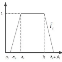
Following the research in (Li and Xu 2013), in this paper, we assume that the turnover rate of assets is simulated as trapezoidal fuzzy numbers. A fuzzy number A is called trapezoidal, denoted as
( , , , )
A a b with tolerance interval [a, b], left width
and right width
, if its membership function takes the following form:1 , ,
1, , ( )
1 , ,
0, a t
if a t a
if a t b A t
t b
if b t b
otherwise
(1)
Let the trapezoidal fuzzy number li( , , , )a bi i i i
(shown in Fig.1) denote the turnover rate of asset i. Then the turnover rate of the portfolio X = {x1, …,
xn } is 1 n
i i i
l x
[image:2.595.372.478.265.370.2]
. We apply the crisp possibilistic mean value of the turnover rate of the portfolio to measure the portfolio liquidity.Fig. 1. The Trapezoidal Fuzzy Membership Function (Li and Xu 2013)
According to (Carlsson and Fullér 2001), the crisp possibilistic mean value (denoted by M) of the fuzzy number defined by the above membership function (1) is calculated as the following:
1
0
( ) ( )
M A
a b d (2)Based on (2) and with the following lemma by (Li and Xu 2013), we can obtain the possibilistic mean value of the turnover rate of the portfolio as a rough estimation for the portfolio’s turnover rate.
Lemma Let the trapezoidal fuzzy number ( , , , )
i i i i i
l a b be the turnover rate of asset i with membership function (1). Then the possibilistic mean value of the turnover rate associated with portfolio X = {x1, …, xn } is
1
( ( )) ( )
2 6
n
i i i i
i i
a b
M l x x
(3)
Proposed Multi-objective Model
1
1 1
2
1
3
1
1
min (4)
max (5)
max ( ) (6)
2 6
. . 1
n n
ij i j
i j
n
i i i
n
i i i i
i i
n
i i
f x x
f r x
a b
f x
s t x
1
min
(7)
(8)
(9) (10)
0 1, {0,1}, 1,
n
i i
i i
i i
i i
z C
x z
x z x
x z i
... (11)n
Objectives (4) (5) and (6) describe risk, return and liquidity of the portfolio that an investor concerns. We assume that the investor does not invest additional capital during the period, i.e., we have a self-financed budget constraint (7). The cardinality constraint (8) restricts the number of assets included in the portfolio. Investors can define the number of assets, C, in the portfolio. n extra binary variables ziare introduced to
indicate if an asset is held or not in the portfolio. zi=1
if the investor hold asset ai (i.e., wi > 0), zi = 0
otherwise. Constraint (9) sets the relation between xi
and zi. The minimum position constraint prevents
investors from holding very small amount of assets. We introduce a prescribed percentage value xmin>0.
That is, holding a position strictly less than xmin is not
advised. Constraints (9) and (10) together ensure this minimum position constraint. Domains of the decision variables are defined by (11).
COMPROMISE BASED GOAL PROGRAMMING APPROACH WITH SATISFACTION FUNCTION
Goal programming (GP) was first introduced in (Charnes, Cooper et al. 1955) and (Charnes and Cooper 1961) as a well-known procedure for solving multi-objective optimisation problems. Many conflicting objectives are taken into account simultaneously in the optimisation. The standard mathematical formulation of the GP model is as follows:
1
min ( )
. . ( ) , 1,...
( ) , 1,...,
, 0, 1,...
m
i i
i
i i i i
k k
i i
s t f x g i m
h x b k K
x D
i m
(12)
where xj is the decision variable. D represents the set of
feasible solutions. hk (x) ≤ bk represents the constraints.
fi is the achievement level of objective i . gi represent
the aspiration level associated with objective i. i and
i
are, respectively, the positive and negative
deviations between the achievement level and the aspiration level. The objective is to minimize the positive and negative deviations.
It is well known in the literature that a solution of a GP model is not necessary a Pareto optimal solution. The GP model produces a solution to a multi-objective problem with a given level of satisfaction. To reduce the computational difficulty of evaluating and selecting the best solution to obtain a Pareto optimal solution, compromised solution can be applied to resolve the conflicting objectives.
Compromise Programming (CP) is a multi-objective decision making technique, proposed in (Zeleny 1973), to obtain compromise solutions. The basic idea is to firstly identify an ideal solution as a point where each single objective under consideration achieves its optimal value. Then it seeks a solution that is as close to the ideal point as possible by minimizing the distance between the achievement level fi (x) and the
ideal values fi* associated with each objective i. The
ideal value fi* for objective i can be obtained by
applying the above GP model (12) for the objective without considering the other objectives. For example, in case of minimizing objective i, the ideal value can be obtained as follows:
* min ( ) 1,...,
. . ( ) , 1,...,
i i
k k
f f x i m
s t h x b k K
x D
(13)
And the CP model can be formulated as follows:
1
*
min
. . ( ) , 1,...
( ) , 1,...,
0, 1,...
m
i i
i i i
k k
i
s t f x f i m
h x b k K
x D
i m
(14)
For our MO-PSP model, we first compute the ideal values V*, R*, and L* for the three objectives by considering the following problems, respectively:
1
1 1
2
1
3
1
min (4)
max (5)
max ( ) (6)
2 6
n n
ij i j
i j
n
i i i
n
i i i i
i i
f x x
f r x
a b
f x
After genera measure the achievement follows: 3 3 ( ) [ ( p Q x w f
where w1 , w
importance o (6), respectiv can use their weights to objectives. p
represents th from the ide weighting of
1( ) 1( 1
Q x w f
yields the so different typ solution for shown in (Li test the cas Investigation Qp(x) remain
With the Q converted to subject to con
Generally we their preferre assumption investment described by and “medium different inv conflicting o over lower r When makin different sen order to inco select the be satisfaction f Aouni 1990)
The degree o maximized t employing t makers are ab
EXPERIME
In this sectio model and solution met FTSE stock
ating the ide quality of a
function, i.
1 1
1/ 3
{[ ( ( ) ( ) *)] }p
w f x f x L
w2, w3 are the
of objective ri vely. It is assu r experience to assign a de
{1,2... }
p de
he importanc eal point. Ty f the deviation
1( ) *) 2
f x V w
o-called Manh pes of metric
convex and c i, Burke et al. se of p=1 ns on differen n our future wo
1(x) metric, t
a single obje nstraints (7)-(
m
e assume that ed values for is usually n market. Usu y the terms suc m liquidity”, vestors have d
objectives. O risk, but the ng the investm nsitivity to th
orporate expl est multi-crit functions, firs .
of satisfaction o provide the the satisfacti ble to explicit
ENTAL RESU
on, we illustr show the eff thod based on market. The
eal solution a feasible solu e. metric Qp
2
*)]p [ (
p
V w f
e weights whi sk (4) return ( umed that the o provide the egree of imp efines the typ
e of the max ypically, as p
ns also increa 2
( ( )f x R*)
hattan metric. in generating concave probl 2012). In thi in the expe nt formulation ork. the MO-PSP ective program (11): 1 min ( )
x Q x
t investors are the objectives not true in ually, these ch as “low risk etc. What is different prefe One may prefe
other may pr ment decisions he deviation o
licitly all of eria portfolio st introduced
of the decisio e most satisfic ion functions tly introduce t
ULTS
rate the prop ffectiveness o n 31 selected historical pr
point, we c ution x with
p(x) defined
2( ) *)]
p
f x R (1
ch represent t (5) and liquid decision mak values for the portance to t pe of metric. ximal deviati p increases, t ases. When p=
3( ( )3 *
w f x L
. The effects g Pareto optim lems have be
s paper, we fi eriment sectio
ns of the met
model is th mming proble
(1
e able to provi s. However, th
the real-wo objectives a k”, “good retu s more, usua erences over t fer higher retu refer lower ri s, investors ha of the goals.
these factors o, we apply t
by (Martel a
on maker will ced solution. B s, the decisi their preferenc
osed simulati of the propos assets from t ice data of 2
can an as 15) the dity ker ese the It ion the =1, ) of mal een irst on. tric hen em 16) ide his rld are urn” ally the urn sk. ave In to the and be By ion ces. ion sed the 261 w co co im CP ha w Pa W tra i l 20 i a ra w ab of 4% an 4% on at in an tu se m ac tu Po In as to th ac re sa ob W th sa
weeks have bee ovariance ma ompromise ba mplemented i PLEX on top ave been carr with CPU @ 3.
arameter sett
We assume th apezoidal
( , , ,a bi i i i
013) to set th
, ,
i bi i and i
ates of the as where its daily bove mentione f the data were %], as shown nd right width %] into small n this, we set t t a=0.5% and nterval at b=2
nd the right w urnover rates
etting of thes may be set to ccording to th urnover rate se
Fig.2. The hi
ortfolio strate
n this section spects of the o different fact he portfolio
chievement ob eturn and liq atisfaction val
bjective.
We will compa he decision ma
atisfaction fun
en collected to atrix and a ased goal pro in C++ with of CPLEX12 ried out on an 16GHz 3.17G
ting
he turnover r fuzzy nu )
i
. We apply he values for , based on th ssets. For ex y turnover rat ed historical d e concentrated in Fig.2. In h, we manually
er intervals fo the left endpo d the right e
.2%. The left width is set a of all 31 sto se four param different valu heir preferenc ets in the follo
istogram of th
egy analysis
n, we compa portfolio strat tors in the mo
strategies bjective value quidity (fi de
ue Fi(δi)of th
are the sensitiv aker’s attitude nctions.
o determine th also turnove
ogramming m h concert te 2.3 solver. Al n Intel Core GHz and 2.97G
rate for the umbers, de the method i r the four pa he histogram xample, we e
tes are collec data. It was fo d around an in order to set t y divided the for every 0.2% oint of the tole
endpoint of ft width is set at =0.8%. S ocks are dete meters is subj ues by individ ces. We will owing sections
he historical tu
are and anal ategies and th odel. Here are we concern es of portfoli efined in (14 he decision m
vity of the abo e expressed b
he return rate, r rate. The model (16) is echnology in l experiments Duo machine GB memory.
assets to be enoted by in (Li and Xu arameters, i.e. s of turnover exam a stock cted from the und that most nterval of [0% the left width interval [0%, % unit. Based rance interval the tolerance t at = 0.4% Similarly, the ermined. The jective. They dual investors test different s. urnover rate lyse different eir sensitivity the aspects of n: (1) The ios, i.e., risk, 4)). (2) The maker for each
The logistic satisfaction function is given by
1 ( )
1 exp( ( ))
i i
i i i
F
s mid
. The functions (i.e. for risk,
return and liquidity) rely on the set of shape parameter values siand the middle satisfaction values midi. We
take two hypothetical situations to test the results. The first situation is that the investor purses an aggressive investment strategy, i.e. prefers higher level returns and liquidity even though it may imply higher risks. Conversely, the second situation is that the investor purses a conservative investment strategy, preferring lower risk even though such a strategy may imply lower return and liquidity. These two situations can be described by the parameter values of
s
iand midi shownin Table 1. The corresponding logistic satisfaction functions with parameters given in Table 1 for risk, return and liquidity are plotted in Figs 3-5.
In Fig.3, function f (200, 0.016) and f (100, 0.016) are satisfaction functions for an aggressive investment strategy with different shape parameters, i.e. srisk =200
and srisk =100 (shown in Table 1.). On the contrary,
[image:5.595.324.532.69.201.2]functions f (200, 0.012) and f (100, 0.012) are from a conservative investment strategy. The middle satisfaction values of functions f (200, 0.016) and f(100, 0.016) is higher than that of f (200, 0.012) and f (100, 0.012). This indicates that f (200, 0.016) and f (100, 0.016) represent an aggressive investment strategy comparing against f (200, 0.012) and f (100, 0.012). The above same philosophy applies to Fig.4 and Fig.5.
Table 1. The attributes of parameters in the logistic satisfaction function Fi(δi)
Aggressive investment strategy
Conservative investment strategy midi midrisk =0.016
midreturn =0.00525
midliquidity =0.7
midrisk =0.012
midreturn =0.002
midliquidity =0.5
si (set 1)
srisk =200
sreturn =2000
sliquidity =40
srisk =200
sreturn =2000
sliquidity =40
si (set 2)
srisk =100
sreturn =1000
sliquidity =10
srisk =100
sreturn =1000
sliquidity =10
[image:5.595.324.530.229.376.2]Fig.3. The logistic satisfaction functions for risk
Fig.4. The logistic satisfaction functions for return
Fig.5. The logistic satisfaction functions for liquidity
For the investor that takes aggressive and optimistic investment strategies, we take the following middle satisfaction values: midrisk= 0.016, midreturn = 0.00525,
and midliquidity = 0.7. The computational results are
[image:5.595.52.286.452.741.2]summarized in Table 2.
Table 2. The portfolio obtained for two aggressive investment strategies (row 1 and row 2) Achievement value Satisfaction value
Risk Return Liquid Risk Return Liquid
0.002627 0.008358 0.8896 1 1 0.796
0.0033352 0.0093586 0.7675 1 1 0.392
For the investor that takes conservative and pessimistic investment strategies, we take the following middle satisfaction values: midrisk= 0.012, midreturn = 0.002,
and midliquidity = 0.5. The computational results are
summarized in Table 3.
Table 3. Portfolio obtained for conservative investment strategies (row 1 and row 2).
Achievement value Satisfaction value
Risk Return Liquid Risk Return Liquid
0.000953 0.006358 0.8489 1 1 1
0.002610 0.008331 0.893 1 0.657 1
A comparison of the solutions listed in Tables 2 and 3 highlights that if the investor chooses an aggressive strategy a higher level of expected return will be obtained than choosing conservative strategy, but with
0 0.2 0.4 0.6 0.8 1 1.2
0 0.01 0.02 0.03 0.04 0.05 0.06
satisfact
ion
va
lu
e
deviation
Logistic satisfaction function for portfolio
risk f(α, mid)
f(200,0.016) f(200,0.012) f(100,0.016) f(100,0.012)
0 0.2 0.4 0.6 0.8 1 1.2
0 0.001 0.002 0.003 0.004 0.005 0.006 0.007 0.008 0.009 0.01
satisfact
ion
va
lu
e
deviation
Logistic satisfaction function for portfolio return f(α, mid)
f(2000,0.00525) f(2000,0.002) f(1000,0.00525) f(1000,0.002)
0 0.2 0.4 0.6 0.8 1 1.2
0 0.5 1 1.5 2
satisfact
ion
va
lu
e
deviation
Logistic satisfaction function for portfolio liquidity f(α, mid)
[image:5.595.309.546.494.540.2] [image:5.595.309.533.648.695.2]a higher ris investor pref the expected lower level ri
Now we ana in (15) on the
Decision ma different wei the structures - Port 4, co weights for t the investor than on liqui on liquidity. compositions see that the s to the weigh that the pre controlled by objective wh section. How are sensitive Fig.6. Com fou
Based on this has the ab judgment (f satisfaction f and to obtai accordance w
CONCLUSI
In this paper portfolio sele namely retu approach ba approach is portfolio s incorporated introduce de from experi
sk level too. fers conservat d portfolio retu
isk too.
alyse the weig e portfolio str
aker can expr ights to indivi s and compos onstructed by the objectives.
assigns highe idity, and in P . Fig.6 illust s of the four p structures of th hts of the obj
eferences of y the satisfac hich will be i wever, the co to the weight
mparison of str ur portfolios d
s we can conc bility to con fuzzy inform functions in th in a satisfacto with the attitud
IONS AND F
r, we propose ection model urn, risk and
ased goal p s proposed
strategy. Sa into the po ecision maker iments that
On the othe tive strategy a urn will be ch
ght to the indi ategy informa
ess his prefer idual objectiv
ition of four p y our model . In Port 1, Po er weights on Port 2 a higher trates the str portfolios. Fro he portfolios a jectives. This objectives ction function investigated i ompositions o s of the object
ructures and co different weigh
clude that the nsider the p mation) by
he portfolio se ory personali des of differen
FUTURE WO
a constrained which include d liquidity. programming to obtain a atisfaction ortfolio select
r’s preference the approach
er hand, if t a lower level hosen but with
vidual objecti ation.
rence by setti es. Fig.6. sho portfolios, Por l with differe
ort 3 and Port n risk and retu
r weight is giv ructure and t om Fig.6 we c are not sensiti may be due are structura ns of individu
n the followi of the portfoli
tives.
ompositions o ht sets.
proposed mod preferences a
employing t election proce sed portfolio nt investors.
ORK
d multi-objecti es three criter A comprom (GP) soluti a compromis functions a tion process es. We obser h can genera
the of h a ive ing ows rt 1 ent t 4, urn ven the can ive to ally ual ing ios of del and the ess, in ive ria, mise ion sed are to rve ate sa at In ju fu Fu po es ac In in fin un un fu se sim st in R Ao Ar Bi Bi Ca Ch Ch Ch Co Cr He atisfactory per ttitudes of diff
n the model, udgement are unctions, whic
uzzy informa ortfolio select stablish prefe chievement fu
n this paper nformation in nancial marke ncertainty pro ncertainty prop uzzy uncertain etting, the multaneously ochastic prog n our future wo
REFERENCE
ouni, B., C. C portfolio ma model: Curr Operational R renas Parra, M.
2001. "A fuz selection." E 133(2): 287-2 ilbao-Terol, A.
V. Rodríg programming Mathematics ilbao, A., M. Ar "On construc European Jo 847. arlsson, C. and
value and va Systems 122( hang, T. J., N.
2000. "Heur optimisation. 1271-1302. harnes, A. and
and industria York, John W harnes, A., W
"Optimal esti programming oupland, S. and Type-2 Fuzz Fuzzy System rama, Y. and M
complex port of Operationa e, F. and R. Q integer progr to portfolio 289:190-205 rsonal portfoli ferent investor the investor’s e explicitly e ch are repres ation is thus tion analysis. erred satisfac unctions.
r, we prima n financial m
et, some vari operties and perties. Becau nty are often portfolio se consider two gramming app
ork.
S
olapinto and D anagement thro ent state-of-the
Research 234(2
, A. Bilbao Ter zzy goal progra European Journ
297.
, B. Pérez-Glad uez-Uría. 20 g for portf and Computati renas, M. V. Ro cting expert Be urnal of Opera
d R. Fullér. 2 ariance of fuzz 2): 315-326.
Meade, J. E. ristics for card " Computers &
W. W. Cooper al applications Wiley and Sons W. W. Cooper imation of exec g." Managemen d R. I. John. 2 zy Logic Syste ms, 15(1):3 - 15. M. Schyns. 20 tfolio selection
al Research 150
Qu. 2014. "A ram modelling
selection prob .
ios in accorda rs.
s preferences expressed by sented by fuz incorporated . The decisio ction level
arily conside market. In a
iables can ex others can e use random un combined in election pro ofold uncertai proach will be
D. La Torre. 20 ough the goal he-art." Europe
2): 536-545. rol and M. V. R amming approa nal of Operati
dish, M. Arena 006. "Fuzzy
folio selectio tion 173(1): 251 odríguez and J. etas for single ational Researc
2001. "On pos zy numbers." F
Beasley and Y dinality constra & Operations R
er. 1961. Manag of linear progr Inc.
and R. O. Fe cutive compens nt Science 2: 13 2007. "Geometr ems." IEEE Tr .
003. "Simulated problems." Eur 0(3): 546-571. A two-stage sto and hybrid sol blems." Inform
ance with the
, attitude and y satisfaction zzy functions. into GP for on maker can for relevant
er the fuzzy complicated xhibit random exhibit fuzzy ncertainty and a real world ocess should inty. A fuzzy e investigated
014. "Financial l programming ean Journal of
Rodrı́guez Urı́a. ach to portfolio ional Research
as-Parra and M. compromise on." Applied 1-264.
Antomil. 2007 -index model." ch 183(2):
827-sibilistic mean Fuzzy Sets and
Y. M. Sharaiha. ained portfolio
esearch 27(13)
gement models ramming. New
erguson. 1955. sation by linear
8-151. ric Type-1 and Transactions on
Fang, Y., K. K. Lai and S.-Y. Wang. 2006. "Portfolio rebalancing model with transaction costs based on fuzzy decision theory." European Journal of Operational
Research 175(2): 879-893.
Fleten, S.-E., K. Høyland and S. W. Wallace. 2002. "The performance of stochastic dynamic and fixed mix portfolio models." European Journal of Operational
Research 140(1): 37-49.
Gaivoronski, A. A., S. Krylov and N. van der Wijst. 2005. "Optimal portfolio selection and dynamic benchmark tracking. "European Journal of Operational Research 163(1): 115-131.
Gupta, P., M. K. Mehlawat and A. Saxena. 2008. "Asset portfolio optimization using fuzzy mathematical programming. "Information Sciences 178(6): 1734-1755. Jobst, N. J., M. D. Horniman, C. A. Lucas and G. Mitra. 2001.
"Computational aspects of alternative portfolio selection models in the presence of discrete asset choice constraints." Quantitative Finance 1(5): 489-501. Kellerer, H., R. Mansini and M. G. Speranza. 2000.
"Selecting Portfolios with Fixed Costs and Minimum Transaction Lots. "Annals of Operations Research 99(1): 287-304.
Li, J., E. K. Burke, T. Curtois, S. Petrovic and R. Qu. 2012. "The falling tide algorithm: A new multi-objective approach for complex workforce scheduling." Omega 40(3): 283-293.
Li, J. and J. Xu.2013. "Multi-objective portfolio selection model with fuzzy random returns and a compromise approach-based genetic algorithm." Information Sciences 220(0): 507-521.
Markowitz, H. M. 1952. "Portfolio Selection." J. Finance 7: 77-91.
Martel, J.-M. and B. Aouni. 1990. "Incorporating the decision maker's preferences in the goal programming model."
Journal of the Operational Research Society 41(12):
1121-1132.
Steuer, R. E., Y. Qi and M. Hirschberger. 2005. "Multiple objectives in portfolio selection." Journal of Financial
Decision Making 1: 11-26.
Zadeh, L. A. 1965. "Fuzzy sets." Information and Control 8(3): 338-353.
Zadeh, L. A. 1999. "Fuzzy sets as a basis for a theory of possibility." Fuzzy Sets and Systems 100, Supplement 1(0): 9-34.
Zeleny, M. 1973. "Compromise Programming." Multiple
Criteria Decision Making:262-301.
AUTHOR BIOGRAPHIES
Fang He was born in China and obtained her PhD degree from The University of Nottingham, U.K. Now she is a Research Fellow working on modelling and optimisation for combinatorial optmisation problem in real-world applications.
Rong Qu is an Associate Professor of Computer Science, at the School of Computer Science, The University of Nottingham, U.K. Her research interests are on the modelling and optimisation algorithms (meta-heuristics, mathematical approaches and their hybridisations) to real-world optimisation and scheduling problems.
Robert John is a Professor of Operational Research and Computer Science. He is the Head of the Automated Scheduling, Optimisation and Planning (ASAP) group in