Empirical Analysis of VDAX and VSTOXX as Major Volatility Indices in the EU Including Forecasting Tools

ISSN Online: 2167-9541 ISSN Print: 2167-9533

DOI: 10.4236/jfrm.2019.84022 Dec. 31, 2019 315 Journal of Financial Risk Management

Empirical Analysis of VDAX and VSTOXX as

Major Volatility Indices in the EU Including

Forecasting Tools

Ernst J. Fahling

, Elmar Steurer

, Manuel Ulbig

, Burkhard Bamberger

1_{International School of Management, Frankfurt am Main, Germany} 2_{Hochschule Neu-Ulm, Neu-Ulm, Germany}

Abstract

This study reviews various time series forecasting models in order to find the best fit for the VDAX and VSTOXX for one month and one year. Addition-ally, the influence of the trading volume of the DAX is examined. Both dura-tions are found to be stationary by the Phillips-Perron test, that is why non-integrated models are used. For a duration of one month, a GARCHX(1,1) model is the best fit in-sample as well as out-of-sample, while the best fit for a duration of one year is found to be a ARX(1) model. Based on the forecasts, two trading strategies are tested for each duration, which is a long only strat-egy and a combination of long and short trades. The performance of both strategies is compared with a simple buy and hold strategy on each VDAX and VSTOXX. It is found that an excess return over the buy and hold strategy can be generated for both durations even with transaction costs.

Keywords

One Year VDAX, VSTOXX Forecasting, ARMA- & GARCH- & ARX-Testing Model, Profitable Trading Strategy

1. Introduction

The forecasting of volatility has received high attention in the econometric lite-rature, due to the fact that financial volatility is usually highly auto-correlated. In an extensive review, Poon & Granger (2003) found 93 published and working papers, which were studying the forecasting performance of various models on realized volatility. Also, in recent literature, the forecasting of realized volatility in financial markets remains a highly studied topic for different equity indices How to cite this paper: Fahling, E. J.,

Steurer, E., Ulbig, M., & Bamberger, B. (2019). Empirical Analysis of VDAX and VSTOXX as Major Volatility Indices in the EU Including Forecasting Tools. Journal of Financial Risk Management, 8, 315-332. https://doi.org/10.4236/jfrm.2019.84022

Received: December 7, 2019 Accepted: December 28, 2019 Published: December 31, 2019

Copyright © 2019 by author(s) and Scientific Research Publishing Inc. This work is licensed under the Creative Commons Attribution International License (CC BY 4.0).

DOI: 10.4236/jfrm.2019.84022 316 Journal of Financial Risk Management and stock exchanges all over the world. For example, Cheng (2015) studied the forecasting performance of implied volatility and a GARCH(1,1) model for the S&P 500. For the Stockholm Stock Exchange, an evaluation of several GARCH type model was done by Dritsaki (2017), while Zhang, De Mello, & Sadeghi (2018) were studying the Australian market. A forecasting study on realized vo-latility for the Dhaka Stock Exchange can be found by Abdullah, Kabir, Jahan, & Siddiqua (2018) and for the Indian market by Shaikh & Padhi (2014). However, the research on the forecasting on volatility indices as a measurement of implied volatility is in comparison to realized volatility rare. In the writing of this paper only one published and one working paper could be found which is studying the forecasting of the VIX index.

Liu, Guo, & Qiao (2015) tested a GARCH(1,1), a GJR GARCH(1,1) and a Heston-Nandi GARCH(1,1) model on the VIX index in-sample and out-of-sample. Out-of-sample all three models on average underestimated the VIX, which was interpreted by the authors as a variance risk premium. A more extensive study on VIX forecasting was done by Ahoniemi (2008), which found the VIX to be non-stationary and therefore used an ARIMA(1,1,1) model with and without GARCH(1,1) errors. Also, she tested both versions with multiple explanatory variables like the trading volume and the return of the S&P 500. All four models were tested out-of-sample via MSPE and modified DM test as well as with a trading strategy. The trading strategy was performed through straddles and a positive average could be earned for all models when no filter was applied. If a filter was applied, signals were left out when the projected change in the VIX was less than 0.1%, 0.2% or 0.5%. With a filter, the return decreased for all models and for a filter with 0.5% even became negative.

Despite from these two studies, Clements & Fuller (2012) used a semi-parametric method to forecast only the sign of the change in the VIX and used it to hedge a long equity position. They found that such a strategy significantly improves the risk-return characteristics of a simple long equity position.

For other volatility indices however no forecasting studies could be found. Stanescu & Tunarus (2012) study incorporates next to the VIX also the VSTOXX but instead of the level the study tries to forecast the spread between both vola-tility indices.

strate-DOI: 10.4236/jfrm.2019.84022 317 Journal of Financial Risk Management gy by applying a trading strategy based on forecasts. However, this trading strategy is only hypothetical since no products on the VDAX could be found by the making of this paper. Although a future market for the VDAX has existed, it was very illiquid and therefore the tradability of the VDAX was very difficult as indicated by Schöne (2009). The present study can therefore be seen as a theo-retical work, which examines how well the VDAX can be predicted by applying a hypothetical trading strategy. Still the results can be used in an equity invest-ment for market timing or portfolio manageinvest-ment. For the VSTOXX, on the other hand, a future market does exist, and the results are also of interest from a practical view.

To predict the levels of the chosen volatility indices standard time series mod-els, like the ARMA model or the GARCH model of Engle & Bollerslev (1986) are chosen. In addition, also the predictive ability of the trading volume of the un-derlying equity index is examined in form of an additional explanatory variable. Most papers only focus on the standard forecasting models and are not consi-dering other factors which could have an influence. In our study, it is found that the trading volume especially out-of-sample leads to a significantly higher fore-casting performance for all chosen indices.

In our study, it is found that the VDAX for one month and one year as well as the VSTOXX are predictable to an extent which makes it possible to generate a significant excess return over a buy and hold strategy, if trading the index is possible.

2. Methodology

This study applies several standard time series forecasting models to model the VDAX and VSTOXX. These forecasting models are auto-regressive-processes (AR) as well as ARMA and GARCH models. All three types of models are also tested with the trading volume of the DAX in million as additional explanatory variable. In this case, an X is added to the name of a forecasting model. As seen in Equation (1), the general form of an ARMAX model is given by:

0 1 1 1 , 1

p q r

t i i t i i i t q i i i t t

y =α +

∑

∑

∑

It can be seen that the ARMAX model contains three sets of explanatory va-riables, which are the AR-lags, described by α times the lagged dependent varia-ble y, the MA lags, described by β times the lagged residuals ε, and a set of addi-tional explanatory variables x times a new parameter ϕ. The ARMAX model is therefore simply an extension of an ARMA model by additional explanatory va-riables. For a GARCHX model, the general form is given by:

2

0 1 1 1 , 1

p q r

t i i t i i i t q i i i t t

y =α +

∑

∑

∑

re-DOI: 10.4236/jfrm.2019.84022 318 Journal of Financial Risk Management siduals ε.

Our forecasting procedure is the following: The parameters of the models are estimated over an entire year and then used for out-of-sample daily forecasts for the following year. Afterwards the parameters are estimated newly for the forth-coming year and again used for daily forecasts of the following year. This pro-cedure continues for the entire data sample. The parameters are estimated by a Maximum Likelihood Estimation (MLE) with the Gaussian Distribution for an in-sample evaluation. For the evaluation and ranking the Schwarz-Bayes infor-mation criterion (SBIC) of Schwarz (1978) is used. The SBIC puts a higher pe-nalty on a high number of parameters than other information criteria and is the most used information criterion in the literature about forecasting volatility. Since the parameters are estimated newly each year, also the SBIC is newly esti-mated each year. Calculating an SBIC for each year shows differences in the in-sample performance of the different models depending on the period and therefore allows for a better comparison of the different models.

The results of the in-sample analysis are used to choose the best three to four models for an out-of-sample analysis. Then all forecasts based on the chosen models are compared by applying the mean squared prediction error (MSPE) as well as the sign test by Diebold & Mariano (1995) and the modified DM test by Harvey, Leybourne, & Newbold (1997). Only if a model is not significantly worse in quality and accuracy than the other chosen models it is used for the fi-nal step in the out-of-sample afi-nalysis, which is a trading strategy.

More interesting from a practical point of view is not a higher accuracy of a model, but if the forecasts based on model can be used for a profitable trading strategy. For this reason, the forecast data of all models which are not sorted out previously is used in two trading strategies, which are a long only and a long-short strategy. In the long only strategy, the VDAX is bought when the forecast predicts a higher VDAX. If the forecast predicts a lower VDAX the po-sition is closed. In the long-short strategy, the VDAX is bought when the fore-cast predicts a higher VDAX and sold when the forefore-cast predicts a lower VDAX, to profit from positive and negative movements. In contrast to Ahoniemi (2008), the average daily return is annualized and then compared with a benchmark. As benchmark a simple buy and hold strategy on the VDAX is chosen, since a trad-ing strategy cannot be considered profitable if it does not generate an excess re-turn over a simple passive investment strategy.

DOI: 10.4236/jfrm.2019.84022 319 Journal of Financial Risk Management value is greater than the transaction cost. This can therefore reduce the number of trades, which is why the transaction costs can also function as a filter.

3. VDAX Analysis

3.1. Data and Calibration

As already stated, two durations for the VDAX are chosen which are one month and one year. The analysis was also made for a duration of three months, six months and two years. However, the trading strategies on these durations did deliver a significantly lower excess return, which is why we chose only the two durations for this paper. All data are obtained from the database Thomson Reu-ters Eikon. For the investigations a data set from the beginning of 2007 until the end of 2018 is chosen. The data set therefore contains a period of 12 years, which includes a period of high volatility concerning the financial crisis, as well with the long bull market afterwards also a period with rather low volatility. Figure 1 gives an overview about the development of the VDAX for both durations in the sample period.

It can be seen that both durations offer a high volatility. The chart of the

DOI: 10.4236/jfrm.2019.84022 320 Journal of Financial Risk Management VDAX for one month shows multiple peaks, with the peak at the peak at the be-ginning of 2018 being the most visible, while the VDAX for one year shows mul-tiple sudden downfalls. If these strong movements can be predicted correctly a high excess return can be generated. On the other hand, there is the threat that these outliers bias the parameter estimation.

A necessary condition for the chosen time series forecasting models is the presence of autocorrelation. Also, the number of significant lags, which need to be included, must be determined in order to calibrate the model as well as possi-ble. To find out the optimal number of AR-lags, Figure 2 shows a partial auto correlogram for both durations.

The partial autocorrelogram shows a high influence of the first lag for both durations. Afterwards the influence decreases drastically, to 0.2 of the second lag for a duration of month and even below 0.2 for a duration of one year. There-fore, only for the VDAX for one month a model which also incorporates the second AR-lag will be tested. For the MA lag the same procedure is done, with the results being presented in Figure 3.

Again, the first lag shows the highest influence also for the MA process and falls of afterwards significantly. In comparison to the AR process however the downfall is less strong and also the second lag shows a negative influence. For the one-month VDAX the second lag reaches almost minus 0.3 and the third lag almost 0.4. It is therefore of interest to test a model which incorporates the second and third MA-lag in-sample. For the one-year VDAX the second MA-lag is as well below minus 0.2 which is why a model which incorporates the second lag will be tested in-sample.

As already said the trading volume of the DAX in million will be used as addi-tional explanatory variable. However, the direction of causality in the relation-ship between trading volume and volatility is not clarified yet. Arguments can be

DOI: 10.4236/jfrm.2019.84022 321 Journal of Financial Risk Management

Figure 3. Partial autocorrelogram MA lags.

given for both sides. Either a high volatility leads to more trade in the stock market and therefore a higher trading volume, or a high trading volume leads to more movement in the price of the underlying and therefore to a higher volatili-ty. To verify that the trading volume has significant predictive power, a MLE re-gression over the entire sample period for an ARX(1) model is performed to test for significance of the trading volume.

The AR(1) lag serves as control variable to test if the information of the trad-ing volume is not already contained in the past value of the VDAX. Table 1 shows the results of this regression.

It can be seen that the trading volume is highly significant at 0.1%-level for the one-month VDAX and significant at a 5%-level for the one-year VDAX. Also, the AR(1) lag is highly significant at a 0.1%-level. Therefore, it can be concluded that the trading volume adds significant information to the prediction model, which is not already included in the past values of the VDAX. This does not necessarily mean that the model is free of multicollinearity, however the signi-ficance of both variables makes multicollinearity unlikely.

The calibration procedures have shown that all three types of explanatory va-riables show a significant influence on the VDAX. However, one last question needs to be answered in order to calibrate the models correctly, which is the question of stationarity. To test if the data is stationary the unit root test by Phil-lips & Perron (1988) was performed. The Null hypothesis of non-stationary data could be rejected at a 5%-level for both durations. Therefore, there is no need to use an integrated model.

3.2. Sample Analysis

DOI: 10.4236/jfrm.2019.84022 322 Journal of Financial Risk Management

Table 1. Significance test of the trading volume.

VDAX Coefficient AR(1) Coefficient Trading Volume

One month 0.905*** 0.0072***

One year 0.984*** −0.0009*

Significance Levels: 0.1%***, 1%**, 5%*.

Table 2. Summary statistics of the SBIC for one-month VDAX.

Model Mean SBIC Standard Deviation Minimum Maximum

ARMA(1,1) 1137.79 209.74 819.66 1549.13

ARX(1) 1131.82 209.95 808.75 1544.21

GARCH(1,1) 1120.21 199.63 818.98 1491.85

ARMAX(1,1) 1135.76 207.31 816.75 1540.81

GARCHX(1,1) 1128.58 198.73 824.87 1497.83

AR(2) 1137.5 210.52 819.66 1551.65

ARMA(2,1) 1141.15 210.55 823.16 1554.48

ARMA(2,2) 1165.62 203.57 823.99 1562.5

ARMA(2,3) 1148.32 210.24 829.4 1564.27

summary statistics of the SBIC for the different models. The minimum of each value is highlighted in green.

Table 2 shows models with only one lag in every explanatory variable perform better than models with multiple lags. In contrast to the autocorrelograms which especially for the MA-lags indicated an influence of the second and third MA-lag are considered to have to many parameters according to the SBIC. All four val-ues are bigger for the AR(2), ARMA(2,1), ARMA(2,2) and ARMA(2,3) model. At least one of each values is minimized by the ARX(1), GARCH(1,1) and GARCHX(1,1) model. These three models are therefore used in the out-of-sample analysis. The ARMA(1,1) and ARMAX(1,1) model however cannot minimize one of the values and will therefore not be used.

DOI: 10.4236/jfrm.2019.84022 323 Journal of Financial Risk Management

Table 3. Summary statistics of the SBIC for one-year VDAX.

Model Mean SBIC Standard Deviation Minimum Maximum

ARMA(1,1) 762.83 197.65 262.24 997.02

ARX(1) 766.1 193.91 268.43 993.94

GARCH(1,1) 744.69 200 268.39 1000.46

ARMAX(1,1) 761.35 200.18 262.74 1000.38

GARCHX(1,1) 748.72 200.2 278.6 1011.51

ARMA(1,2) 764.3 198.54 264.34 1005.38

ARMA(1,3) 768.68 197.78 270.9 1007.76

Before the out-of-sample performance of the different models will be com-pared with hypothesis tests and a trading strategy a general overview about the development of the forecasts in comparison to the actual value is given in Figure 4.

For the one-month VDAX it can be seen that the predicted values of the three chosen models are very close to the actual value. Sometimes there is an under- or overvaluation. However, there is no pattern in these errors’ observable. The peak at the beginning of 2018 shows an interesting behavior of the GARCH and GARCHX model. It can be seen that, while the ARX model predicts the high in-crease rather well, the predicted values of the GARCH and GARCHX model af-terwards, due to the high error before becoming negative.

For the one-year VDAX a clear difference between the forecasts of the ARMA model and the other chosen models can be observed. While the GARCH, ARMAX and ARX model are very close to the actual value, the ARMA model shows a consistent overvaluation for multiple years. The other three models are also able to predict sudden downfalls in the VDAX for one year, but this leads to a peak value of the GARCH model afterwards in 2015 and the beginning of 2018.

3.3. Forecasting Quality

Before the results of the sign test and modified DM test are given, Table 4 will give the MSPE of the different models to give a first idea about the accuracy of the different models.

Table 4 shows a significantly lower MSPE of the ARX model in comparison to the GARCH and GÀRCHX model for the one-month VDAX. This might be due to the bias after the peak in the beginning of 2018, which could be seen in Figure 4. The MSPE of the GARCH and GARCHX model, on the other hand, are rather close to each other.

DOI: 10.4236/jfrm.2019.84022 324 Journal of Financial Risk Management

Figure 4. Forecasts and actual value in comparison.

Table 4. MSPE for chosen models.

Model One month One year

GARCH(1,1) 59.33 1.74

GARCHX(1,1) 52.06

ARX(1) 16.6 1.77

ARMA(1,1) 5.73

ARMAX(1,1) 1.65

MSPE is generated by the ARMAX model. However, the MSPE of the GARCH and ARX model is just slightly higher.

DOI: 10.4236/jfrm.2019.84022 325 Journal of Financial Risk Management a greater quality of the forecasts based on the GARCH model than the ARX and GARCHX model cannot be rejected at a 5%.

For the one-year VDAX the null hypothesis of no qualitative difference be-tween the ARMA model and the other chosen models not surprisingly can be rejected at a 5%-level. The one-sided test also rejects the null hypothesis of a greater quality of the ARMA model. Despite the small difference in MSPE of the other chosen models the null hypothesis can be rejected at a 5%-level. The hy-pothesis of a bigger quality of the ARX model in comparison to the GARCH and ARMAX model can be rejected at a 5%-level, while the hypothesis of a bigger quality of the GARCH model in comparison to the ARMAX model cannot be rejected at a 5%-level.

By applying the modified DM test for forecasting accuracy, the null hypothe-sis of no difference in forecasting accuracy cannot be rejected at a 5%-level for any comparison of the chosen models for the one-month VDAX. For the one-year VDAX the null hypothesis of no difference in forecasting accuracy be-tween the ARMA model and the other chosen models can be clearly rejected at a 5%-level. However, by applying the one-sided version of the test, the null hypo-thesis of a higher forecasting accuracy of the ARMA model cannot be rejected at a 5%-level. For the comparisons of the other models the two-sided null hypothe-sis cannot be rejected at a 5%-level.

The results of this chapter have shown that despite a difference in MSPE and quality no significant difference in forecasting accuracy could be found. Only for the ARMA model a significant difference was found by using the modified DM test. Surprisingly the null hypothesis of a higher forecasting accuracy, despite the tendency to overvaluation, cannot be rejected. Therefore, all models which were used for the out-of-sample forecast are also compared in their performance for a trading strategy.

3.4. Results Trading Strategy

DOI: 10.4236/jfrm.2019.84022 326 Journal of Financial Risk Management

Table 5. Annual mean return and confidence level vs Buy & Hold strategy for one-month

VDAX.

Strategy No transaction costs Transaction costs of 0.1% Transaction costs of 0.5% Buy and hold 10.7%

GARCH 11.5%/96.7% 11.3%/97.7% 11.1%/95.8%

GARCHX 11.9%/96.6% 11.5%/96% 11.4%/97.4%

ARX 11.1%/97.3% 11.1%/96.5% 11.2%/97%

GARCH (short) 12.3%/65.9% 13.1%/73.2% 14.2%/80.3%

GARCHX (short) 13%/72.7% 12.8%/69.9% 14.5%/82%

ARX (short) 11.5%/58.3% 11.8%/60.2% 13.5%/74.6%

difference between current value and forecast is more than the transaction costs. Therefore, some movements have been left out in a scenario with transaction costs. If in these cases the forecast has predicted the direction wrong, filtering these movements out can increase the average return.

For the one-year VDAX the results of both trading strategies can be seen in Table 6.

For the one-year VDAX also every chosen forecasting model leads to an excess return over the buy and hold strategy, when applied in a trading strategy. Even the ARMA model leads to an excess return with both trading strategies and under all scenarios, despite the clear tendency to overvaluation. However, the excess return generated by the ARMA model is significantly lower than the other models and in contrast to the other models it the ARMA model does not take advantage from the filter effect of the transaction costs. For the other models, this filter effect is clearly visible, especially in the long short strategy.

In a long only strategy, the ARX model takes a small lead over the ARMAX model in all three scenarios. The GARCH model is in this case clearly outper-formed by the other two models. In the long short strategy, the ARX model also takes the lead in a scenario with no transaction costs or transaction costs of 0.1%. However, under transaction costs of 0.5% the ARMAX and GARCH mod-el can take a better advantage of the filter effect than the ARX modmod-el, which now only takes third place. The first place is now taken by the ARMAX model which in this scenario generates the highest return in Table 6 with 10.3% or an excess return of 7.3%.

The confidence levels show that for the one-month VDAX, it can be said with a confidence of more than 95% that the returns are different from the buy and hold strategy for long term only. By adding short trades, the confidence level de-creases highly at first, but inde-creases with transaction cost of 0.5% to on average 80%. For the one-year VDAX for both strategies the average confidence level is above 90%, except for the ARMA model. This highlights again the bad perfor-mance of the ARMA model.

DOI: 10.4236/jfrm.2019.84022 327 Journal of Financial Risk Management

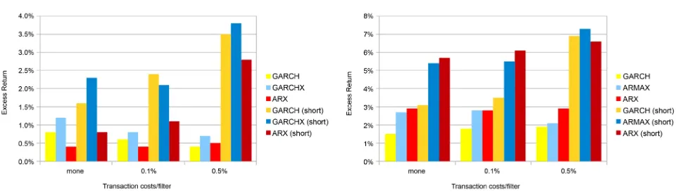
Figure 5. Excess return for one month and one year, related to VDAX.

Table 6. Annual mean return and confidence level vs. Buy & Hold strategy for one-year

VDAX.

Strategy No transaction costs Transaction costs of 0.1% Transaction costs of 0.5% Buy and hold 3%

GARCH 4.5%/87.7% 4.8%/91.2% 4.9%/94.5%

ARMAX 5.7%/98% 5.8%/98.5% 5.1%/96.9%

ARX 5.9%/98.2% 5.8%/98.1% 5.9%/98.6%

ARMA 3.6%/66.5% 3.6%/66% 3.5%/64.4%

GARCH (short) 6.1%/95.2% 6.5%/96.3% 9.9%/99.9%

ARMAX (short) 8.4%/99.8% 8.5%/99.8% 10.3%/100%

ARX (short) 8.7%/99.9% 9.1%/99.9% 9.6%/100%

ARMA (short) 4.2%/74% 4.2%/74% 4.2%/72.6%

a better overview about the generated outperformance. The ARMA model was excluded for this analysis, since the other models have shown to be clearly supe-rior for a duration of one year.

Figure 5 shows that also the excess return over the buy and hold strategy can be significantly increased by adding short trades and that the long only strategy profits a lot from the applied filter for transaction costs. For a duration of one month the highest excess return is generated by the GARCHX model with 3.8%, while for a duration of one year the ARMAX model generates the highest excess return with 7.3%. Both excess returns can only be generated when long and short trades as well as the filter of 0.5% are applied.

DOI: 10.4236/jfrm.2019.84022 328 Journal of Financial Risk Management

4. VSTOXX Analysis

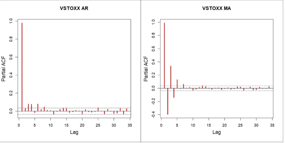
Like for the VDAX for one month and one year the null hypothesis of a non-stationary time series could be rejected for the VSTOXX at a 5%-level. Therefore, non-integrated forecasting models can also be used for the VSTOXX. To decide which number of lags can be used a partial autocorrelogram is drawn for AR and MA processes. These can be seen in Figure 6.

It can be seen in Figure 6 that only the first AR-lag has a significant influence. For the MA-lags on the other hand also the second and third lag show a high in-fluence. Also, a regression with an ARX model was performed to test for the sig-nificance of the trading volume of the Euro Stoxx 50 as predictor for the future VSTOXX. However, in contrast to the VDAX the trading volume did not prove to be a significant predictor of the future VSTOXX. But since models which in-cluded the trading volume as additional explanatory variable performed very good out-of-sample for the VDAX, these models are tested out-of-sample for the VSTOXX as well.

Based on this information and decision all suitable and chosen models are tested in-sample first by applying the SBIC. The results can be seen in Table 7.

As can be seen in Table 7 that the GARCH model can minimize three of the four summary statistics and therefore is on average the best fit in-sample. The ARMA(1,1) model follows closely and can also achieve the lowest minimum value over all tested models. By adding more MA-lags again a decrease in per-formance can be observed. Therefore, also for the VSTOXX the inclusion of more than one MA-lag is not advantageous. For the models which include the trading volume the ARX model can achieve the lowest mean and minimum value, while the GARCHX model can minimize the standard deviation and maximum

DOI: 10.4236/jfrm.2019.84022 329 Journal of Financial Risk Management

Table 7. Summary Statistics of SBIC for VSTOXX.

Model Mean Standard deviation Minimum Maximum

ARMA(1,1) 999.46 169.53 780.31 1387.4

ARX(1) 1003.21 169.6 784.96 1391

GARCH(1,1) 996.9 163.45 783.17 1356

ARMAX(1,1) 1009.14 169.46 791.11 1397.44

GARCHX(1,1) 1006.48 163.71 793.65 1367.3

ARMA(1,2) 1020.95 171.9 822.15 1392.66

ARMA(1,3) 1004.47 171.76 783.86 1403.06

value. The ARMAX model does not show any superiority in one value in com-parison to the other models and is therefore not included in the out-of-sample evaluation. In general, all models which include the trading volume show a weaker performance in comparison to the GARCH and ARMA(1,1) model. Still the GARCHX and ARX model are included in the out-of-sample evaluation due to their high performance for the one-month and one-year VDAX.

In the out-of-sample comparison the four chosen models show no high dif-ference in accuracy when the MSPE is applied. All four models are here in a range of 3.84 to 3.95. If, however, the sign test is applied, the null hypothesis of no qualitative difference can be rejected at 5%-level for the comparison between GARCH and ARX model and GARCHX and ARX model. For all other compar-isons the null hypothesis cannot be rejected at a 5%-level. The one-sided test for the comparison between GARCH and ARX model and GARCHX and ARX model results in a significantly greater quality of the forecasts based on the ARX model, than the GARCH and GARCHX model at a 5%-level. Moving on to the modified DM test the null hypothesis of no difference in accuracy can only be rejected for the comparison between ARX and GARCHX. The one-sided version results in a significantly better accuracy of the ARX model in comparison to the GARCHX model. Therefore, only the ARMA, GARCH and ARX model are used for the trading strategy, with the results being displayed in Table 8. All trading strategies were made under the same assumptions as for the VDAX.

DOI: 10.4236/jfrm.2019.84022 330 Journal of Financial Risk Management Table 8. Annual mean return for VSTOXX.

Strategy No transaction costs Transaction costs of 0.1% Transaction costs of 0.5% Buy and hold 3.7%

ARMA 3.9%/84.8% 4%/85.5% 3.8%/86.4%

GARCH 4.8%/94% 4.7%/93.9% 4%/92.9%

ARX 5.9%/99% 5.7%/98.8% 5.2%/98.2%

ARMA (short) 4.2%/59.2% 4.5%/63.9% 6.1%/86.3%

GARCH (short) 5.9%/85.1% 6.1%/88% 8.2%/98.3%

ARX (short) 8.1%/98.4% 7.8%/97.8% 8.9%/99.4%

Figure 7. Excess return for the VSTOXX, one year.

The excess return which can be generated shows high similarities to the re-sults for the VDAX for one year and one month in its characterizations. Again, the highest excess return is generated with a combination of long and short trades and the filter effect of transaction costs of 0.5%. Although the trading vo-lume was not significant in-sample, the ARX model delivers a clear outperfor-mance out-of-sample with the highest excess return in each scenario. With a long short combination and trading cost of 0.5% the highest overall excess re-turn of 5.2% is generated.

In conclusion, it can be said, that also for the VSTOXX a significant excess return can be generated by applying forecasting models. Like for the VDAX also for the VSTOXX the return can be increased by adding short trades and a clear positive effect of transaction costs as a filter is observable. Also, the best per-forming model again includes the trading volume as additional explanatory va-riable. However, since these results do not include potential rolling costs or li-quidity problems of the VSTOXX futures it is questionable if this performance is fully realizable.

5. Conclusion

DOI: 10.4236/jfrm.2019.84022 331 Journal of Financial Risk Management as well as the VSTOXX are predictable to an extent, which makes it possible to generate high excess returns if the forecasts are used for a trading strategy. Even when trading costs are considered a positive excess return can be generated. The different forecasting models have also proven to predict positive as well as nega-tive movements good enough that not only long, but also short trades could be used to boost the performance even further. Unfortunately, a future market for the VDAX does not exist at the moment, that is why the VDAX cannot be traded as an asset. For the VSTOXX, on the other hand, a future market does exist.

According to the results, the best forecasting model for the one month VDAX is a GARCHX(1,1) model. This model generated under almost each scenario the highest return. For the one year VDAX, the highest return in the long only strategy is generated by an ARX(1) model. If, on the other hand, also short trades are used, it is not completely clear from the results if an ARMAX(1,1) model or an ARX(1) model should be used. There remains a question of the transaction costs and the right filtering. For the VSTOXX, an ARX model was found to be the best fit under each scenario for both strategies. Another conclu-sion, which can be taken from these results is that the trading volume is an im-portant predictor of the VDAX and the VSTOXX, since the best performing models all included it as additional explanatory variable.

The results can be used in further research in three main areas, with the first area being the improvement of the forecasts by using different distributions for the MLE or by using different models. As a second topic, more realistic trading strategies based on reproduction by applying derivatives could be tested. As a possible third topic, the relationship between an equity investment and a trading strategy on the VDAX or VSTOXX could be examined. Here the question is if such a strategy would reduce the risk and increase the return in comparison with a static investment.

Conflicts of Interest

The authors declare no conflicts of interest regarding the publication of this pa-per.

References

Abdullah, S. M., Kabir, M. A., Jahan, K., & Siddiqua, S. (2018). Which Model Performs Better While Forecasting Stock Market Volatility? Answer for Dhaka Stock Exchange (DSE).Theoretical Economics Letters, 8, 3203-3222.

https://doi.org/10.4236/tel.2018.814199

Ahoniemi, K. (2008). Modeling and Forecasting the VIX Index. Helsinki: Helsinki School of Economics, Department of Economics.https://doi.org/10.2139/ssrn.1033812

Cheng, J. (2015). Volatility Forecasting and Volatility Risk Premium. Journal of Applied Mathematics and Physics, 3, 98-102.https://doi.org/10.4236/jamp.2015.31014

DOI: 10.4236/jfrm.2019.84022 332 Journal of Financial Risk Management

Diebold, F. X., & Mariano, R. S. (1995). Comparing Predictive Accuracy. Journal of Busi-ness & Economic Statistics, 13, 253-263.

https://doi.org/10.1080/07350015.1995.10524599

Dritsaki, C. (2017). An Empirical Evaluation in GARCH Volatility Modeling: Evidence from the Stockholm Stock Exchange. Journal of Mathematical Finance, 7, 366-390.

https://doi.org/10.4236/jmf.2017.72020

Engle, R. F. (1982). Autoregressive Conditional Heteroscedasticity with Estimates of the Variance of United Kingdom Inflation. Econometrica, 4, 987-1007.

https://doi.org/10.2307/1912773

Engle, R. F., & Bollerslev, T. (1986). Modeling the Persistence of Conditional Variance.

Econometric Reviews, 1, 1-50.https://doi.org/10.1080/07474938608800095

Harvey, D., Leybourne, S., & Newbold, P. (1997). Testing the Equality of Prediction Mean Squared Errors. International Journal of Forecasting, 13, 281-291.

https://doi.org/10.1016/S0169-2070(96)00719-4

Liu, Q., Guo, S., & Qiao, G. (2015). VIX Forecasting and Variance Risk Premium: A New GARCH Approach. North American Journal of Economics and Finance, 34, 314-322.

https://doi.org/10.1016/j.najef.2015.10.001

Phillips, P. C. B., & Perron, P. (1988). Testing for a Unit Root in Time Series Regression.

Biometrika, 75, 335-346.https://doi.org/10.1093/biomet/75.2.335

Poon, S. H., & Granger, C. W. J. (2003). Forecasting Volatility in Financial Markets: A Review. Journal of Economic Literature, 41, 478-539.https://doi.org/10.1257/.41.2.478

Schöne, A. (2009). Zur Handelbarkeit der Volatilitätsindizes VDAX und VDAX-New der Deutsche Börse AG. Schmalenbachs Zeitschrift für Betriebswirtschaftliche Forschung, 61, 881-910.https://doi.org/10.1007/BF03373672

Schwarz, G. (1978). Estimating the Dimension of a Model. The Annals of Statistics, 6,

461-464.https://doi.org/10.1214/aos/1176344136

Shaikh, I., & Padhi, P. (2014). The Forecasting Performance of Implied Volatility Index: Evidence from India VIX. Economic Change and Restructuring, 47, 251-274.

https://doi.org/10.1007/s10644-014-9149-z

Stanescu, S., & Tunaru, R. (2012). Investment Strategies with VIX and VSTOXX. SSRN Electronic Journal. Advance Online Publication.https://doi.org/10.2139/ssrn.2351427