Evolutionary squeaky wheel optimization: a new framework for analysis

Jingpeng Li

NG8 1BB, United Kingdom

Andrew J. Parkes

School of Computer Science, The University of Nottingham, Nottingham, NG8 1BB, United Kingdom

Edmund K. Burke

School of Computer Science, The University of Nottingham, Nottingham, NG8 1BB, United Kingdom

Abstract

Squeaky wheel optimization (SWO) is a relatively new metaheuristic that has been shown to be effective for many real-world problems. At each iteration SWO does a complete construction of a solution starting from the empty assignment. Although the construction uses information from previous iterations, the complete rebuilding does mean that SWO is generally effective at diversification but can suffer from a relatively weak intensification. Evolutionary SWO (ESWO) is a recent extension to SWO that is designed to improve the intensification by keeping the good components of solutions and only using SWO to reconstruct other poorer components of the solution. In such algorithms a standard challenge is to understand how the various parameters affect the search process. In order to support the future study of such issues, we propose a formal framework for the analysis of ESWO. The framework is based on Markov chains, and the main novelty arises because ESWO moves through the space of partial assignments. This makes it significantly different from the analyses used in local search (such as simulated annealing) which only move through complete assignments. Generally, the exact details of ESWO will depend on various heuristics; so we focus our approach on a case of ESWO that we call ESWO-II and that has probabilistic as opposed to heuristic selection and construction operators. For ESWO-II, we study a simple problem instance and explicitly compute the stationary distribution probability over the states of the search space. We find interesting properties of the distribution. In particular, we find that the probabilities of states generally, but not always, increase with their fitness. This nonmonotonocity is quite different from the monotonicity expected in algorithms such as simulated annealing.

Keywords

Combinatorial optimization, metaheuristics, stochastic search, stochastic process, Markov chain.

1

Introduction

discrete decision variables,denotes a set of constraints among the variables, andf denotes an objective functionf :S→Z+to be maximized (or minimized). Many such problems arising in various fields (such as computer science, management, engineer-ing, etc.) cannot be solved exactly within reasonable time limits for problem instance sizes of practical interest. Heuristics attempt to achieve a trade-off between solution quality and search completeness. Metaheuristic approaches have been widely stud-ied (Gendreau and Potvin, 2010) and can be applstud-ied, with suitable modifications, to a broad class of combinatorial optimization problems. Some well-known examples of metaheuristics are ant colony optimization (Dorigo et al., 1996), estimation of distribu-tion algorithm (Larra ˜naga and Lozano, 2002), stochastic local search (for a review, see Hoos and Stutzle, 2005), genetic algorithms (Goldberg, 1989), GRASP (Feo and Resende, 1989), simulated annealing (Kirkpatrick et al., 1983), TABU search (Glover, 1989), and variable neighborhood search (Hansen and Mladenovi´c, 1999). Based on their method for building new solutions, metaheuristics can be roughly grouped into the following two classes: constructive metaheuristics and iterative metaheuristics. The former gen-erates a solution from scratch by successive addition of certain components (with or without backtracking), whilst the latter starts with a complete solution and changes this solution in an iterative process in order to improve the objective function value.

Among many metaheuristics reported in recent years, squeaky wheel optimization (SWO; Joslin and Clements, 1999) is relatively little known but is receiving increased attention in the research community. This method is based on the observation that in real world combinatorial problems, the solutions consist of components which are intricately woven together in a nonlinear, nonadditive fashion. To deal with these com-ponents, Joslin and Clements (1999) proposed the original idea of SWO, and applied it to production line scheduling problems and graph coloring problems with some satisfactory results. Since then, SWO has been successfully applied to many different types of discrete optimization problems, such as game playing of contract bridge (Gins-berg, 2001) air force space–ground communications (Barbulescu et al., 2004), examina-tion time-tabling (Burke and Newall, 2004), crane scheduling (Lim et al., 2004), port space allocation (Fu et al., 2007), bandwidth multicoloring (Malaguti and Toth, 2008), machine scheduling (Feng and Lau, 2008), and two dimensional strip packing (Burke et al., 2010).

In SWO, an initial solution is first constructed by a greedy algorithm. The solution is then analyzed to assign blame to the components which cause trouble in the solution, and this information is used to modify the priority order in which the greedy algorithm constructs the new solutions. This construction-analysis-prioritization cycle continues until a stopping condition is reached. Hence, the SWO cycle has the consequence that problem components that are hard to handle tend to rise in the priority queue, and components that are easy to handle tend to sink. In essence, this method finds good quality solutions by searching in two spaces simultaneously: the traditional solution space and the new priority space.

on two manpower scheduling problems: driver scheduling (Li and Kwan, 2003) and nurse scheduling (Aickelin and Li, 2007). To achieve this, evolutionary SWO (ESWO) incorporates two additional operators into the cycle: Selection and mutation. The se-lection operator determines whether a component should be discarded and placed in a queue for the new allocation, based on the local fitness of this component. The mutation step further discards some randomly selected components.

We also note that apart from introducing the selection and mutation operators, ESWO did not include the notion from SWO of the sorting of the constructor’s priority queue (PQ) being sticky. Specifically, in SWO, the priority queue is not totally rebuilt at each iteration, but rather it uses the analysis stage to modify the PQ so as to form a new PQ that still preserves some memory of the previous PQ. For example, the items in the PQ might be limited in how far they move within the queue. In contrast, in ESWO, the constructor does not use the results of the previous iteration other than the state that it gives. This means that, although sharing some common motivations, it is rather a different algorithm from SWO. It is perhaps more akin to the many metaheuristics that use some form of iterative repair that identify flaws in a solution, and then attempt to repair them. However, the lack of memory of the previous PQ also means that it is more straightforward to build a Markov chain model based on the search space, and without having to also include the PQ as would (presumably) be necessary to model SWO.

At this point, we explore the motivations to set up studies of the properties of the algorithm. We are inspired, of course, by the numerous Markov Chain analyses of simulated annealing, SA (Michiels et al., 2007). On the technical side, the formulation itself differs from such analyses of SA because ESWO moves through states that are only partial assignments, that is, not all the variables are assigned values. In contrast, local search methods such as SA deal only with states corresponding to complete assignments; all variables are assigned values. However, we note that an increasing number of algorithms do have such movement through the space of partial assignments and thus this class of formulations might well be of increasing interest.

The practical motivation for a formal framework and (semi-empirical) analysis is to be able to better understand the interplay of the various stages within an ESWO algorithm. This is perhaps even more important than for SA, because ESWO is a multi-stage algorithm with potentially many parameters, and it is far from understood how the stages interact with each other.

A challenge in setting up a framework and analysis is that in practice ESWO often contains greedy heuristics with some random factors (e.g., breaking ties randomly). To overcome this drawback, in this paper, we study a particular version of ESWO, that we call ESWO-II, and that is set up to capture (as much as possible) the intent of ESWO, but to do so using stochastic methods that are susceptible to Markov chain anal-ysis. For example, for ESWO-II, we revised the construction step to make probabilistic choices among various possible destination states, though again with a bias toward fitter solutions.

Using a small but concrete example, we then make explicit calculations of the resulting probability distributions over the states. We find that the distributions could be concentrated on the good solutions—this is expected as it would probably not be a good search method otherwise. However, we do find the slightly surprising result that the probability need not vary monotonically with the fitness; sometimes states with slightly lower fitness can be more probable than those with higher fitness. This is in stark contrast to standard methods such as simulated annealing in which the equilibrium (metropolis) distribution is monotonic with respect to fitness. This property of ESWO-II might be regarded as strange, but need not be a bad sign for its effectiveness: After all, it is hitting times that matter more than final stationary distributions. The interaction between such stationary distributions and the hitting times might well be an interesting topic for future research.

Our general motivation for carrying out this study is that the Markov chain numeri-cal solution of smaller instances can allow much faster and more precise numeri-calculation than simulation would give. This then enables a more effective study aimed at understanding how the various components within the algorithms interact with key measures such as stationary distributions. That is, the goal is to explore and understand the interactions of the various components within the search algorithm(s).

The remainder of the paper is structured as follows. Section 2 gives a short intro-duction into the key concepts of finite Markov chains. Section 3 elaborates a formal framework of the ESWO-II, from the state transition point of view. Section 4 presents some mathematical convergence results, and Section 5 discusses some results on sta-tionary distribution. Section 6 contains concluding remarks and some possible future work.

2

Standard Preliminaries of Finite Markov Chains

In this section, we summarize various standard definitions and results that we will need later. A Markov chain is a stochastic process with the Markov property (Tijms, 2003). Being a stochastic process means that state transitions are probabilistic. The Markov property means that the present state is all that is needed to determine the next state. Let{Xn, n=0,1, ...}be a sequence of random variables with state spaceS. A discrete-time Markov chain is defined as

Pr{Xn₊1=in₊1|X0=i0,..., Xn=in} =Pr{Xn₊1=in₊1|Xn=in}. (1)

At each step, the system may change its state from statei∈Sto statej ∈S accord-ing to a probability distribution. The changes of state are called transitions, and the probabilities associated with various state changes are called transition probabilities. If state spaceSis a finite set, the transition probability distribution can be represented by a transition matrixP, with its (i,j)th entry equal to

pij =Pr{Xn₊1=j|Xn=i}, i, j ∈S. (2)

Sincepij ∈[0,1] and

the distribution of the chain after t steps can be obtained by P(t)_=P(0)_Pt_{. Hence, a} homogeneous finite Markov chain {Xn, n=0,1, ...}is completely determined by the initial stateX₀and transition matrixP.

To understand the long-term behavior (or the limit behavior) of the Markov chain

{Xn}, we first give some (standard) definitions as follows.

DEFINITION1: A nonnegative square matrixAis said to be regular if there exists k such that

for all i and j, the (i, j)th entry ofAk_{is positive. (This simply means that for any pair of states}

some sequence of transitions exists between them.)

DEFINITION2: A probability distributionπ =(π₁, π₂, ...)is said to be stationary for a

tran-sition matrix if it does not change after a round of trantran-sitions, that is, with P =(pij)then

πj =

i_∈Sπipij,∀j ∈S.

DEFINITION3: A set of states C is said to be closed if and only ifp(_ikn)|i∈C,k∈C for all n and

j∈Cpij =1for everyi∈C.

DEFINITION 4: A finite Markov chain is said to be irreducible if it does not contain any

non-empty closed subset of states other than the entire state space S. Chains that are not

irreducible are said to be reducible.

DEFINITION5: A Markov chain is said to be aperiodic if and only if the corresponding transition

matrixPis regular.

DEFINITION6: A state i has period k if any return to state i must occur in multiples ofktime

steps. Ifk=1, then the state is said to be aperiodic.

The following well-known result sets up the foundation of our convergence analysis for the ESWO-II algorithm.

THEOREM1: (See, e.g., Koralov and Sinai, 2007.) Given a Markov chain with an ergodic

matrix of transition probabilities P, there exists a unique stationary probability distribution

π =πi. The n-step transition probabilities converge to the distributionπ, that islim

n→∝p

(n)

ij =πj.

The stationary distribution satisfiesπj >0for allj ∈S.

REMARK: The above results can be extended to reducible Markov chain with a single

closed set. Note that the meaning of an ergodic matrix is identical to the regular matrix defined in Definition 1.

3

A Formal Framework for the ESWO-II Algorithm

3.1 State Transitions by the ESWO-II Algorithm

Five operations are performed in sequence at each iteration of the ESWO-II algorithm. They are analysis, selection, mutation, prioritization and construction. The first anal-ysis operation does not alter the current state on its own, as it simply serves as an agent to collect inherent information, in particular the local fitness values of individual components, of the current state.

The second operator, selection, uses the result of the preceding analysis operator and changes the present state by removing the set of selected components from the current solution. However, it does not generate a destination state which is defined as a complete assignment of all components. Hence, we refer to the state after the selection as an intermediate state. Whenever no component has been selected, the intermediate state remains the current state. However, if one or more components have been selected, the intermediate state is an incomplete assignment together with a set of unassigned components. As the selected components are removed, the exact information about the source assignment is thus lost. All possible destination states with the same complete assignments, including the original source, are treated uniformly as seen from the intermediate state. Let x be a source state, and x be an intermediate state. For the selection operator, we write its transition probability from x to x as p_S(Xn+1=x|Xn=x), orpS(x|x) for short.

The third operator, mutation, changes the present intermediate state by further removing the set of mutated components from the current (partial) solution. Like the selection operator, it does not generate a destination state. Hence, the state after mutation remains an intermediate state. Likewise, all destination states with the same complete assignments are treated uniformly as seen from the current intermediate state. Letxbe a previous intermediate state, andxbe a present intermediate state. For the mutation operator, we write its transition probability fromxtoxasp_M(Xn₊1=x|Xn=x), or p_M(x|x) for short.

The fourth operation, prioritization, would not directly alter the present inter-mediate state on its own, but simply use the information of the analysis operator to create the priority order in which the construction operator builds new solutions. However, it is only used in ESWO and not ESWO-II and is only included here for completeness.

The fifth operator, construction, in ESWO-II finally generates a new destination state from the present intermediate state by carrying out probabilistic choices among different possible destination states. In comparison, in ESWO, for construction, the pri-ority order would be used along with partially deterministic algorithms, e.g., greedy heuristics that break ties randomly. Letxbe an intermediate state, andx be a desti-nation state. For the construction operator, we write its transition probability fromx toxasp_C(Xn₊1=x|Xn=x), orpC(x|x) for short.

Assume a solution x(j) _{∈S consists of m componential variables x}

i, denoted as x(j)_=(x

1, ..., xm)(j), and eachxi may take one of thenvalues, that is,xi ∈ {j(

i)

1 , ..., j (i)

n }.

Thenvalues for each variable are not essential but simplify the equations. A variable instantiation, that is, the assignment of a valuej_k(i)to a variable, is denoted byxi =j(

i)

k .

A solutions∈S is a complete assignment in which each variable has a domain value assigned, regardless of the satisfiability on constraint set.

The selection operator can be regarded as a linear map from spaceSof cardinality nm to space S# of cardinality (n+1)m_{, as each variable x}

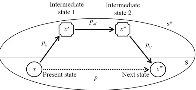
Figure 1: State transition graph of the ESWO-II algorithm.

later when it is marked as selected. That is, a mix of # and non-# symbols is a partial assignment rather than a complete assignment.

At each iteration of the ESWO-II algorithm, a state transition is carried out from a source state to a destination state (as shown in Figure 1). This corresponds to a one-step move in the state graph. We can see that, given a present state, the probability of being in a future state is conditionally independent of the past states. Hence, each step of transitions between complete states has Markov properties.

After defining the state transitions of selection, mutation, and construction, we are able to give an expression for the overall transition probability between any two connected states. We formulate the transition probability from the source statexto the destination statex, via two intermediate states ofxandx, as

p(x|x)=p_S(x|x)·p_M(x|x)·p_C(x|x). (3)

Equation (3) forms the basis for our following Markov chain analysis. We aim to de-rive some global convergence properties and trace a stationary probability distribution, for an insight into the working of the ESWO-II algorithm.

3.2 The Running Example

Throughout this paper, in order to explicitly illustrate the formalism and also to provide empirical results, we use a single running example using just three 0/1 variables xi. The search spaceShas 23_{=8 states, and the intermediate spaceS}#_{has 3}3_{=27 states.} We use a superscript in parentheses to index the search spaceS, and will use the fixed numeric order [000,001,010,011,100,101,110,111] so that in this casejis actually just one plus the numeric value of the string when regarded as a binary number. Hence, in this case, a solutionx(j)_{withj ∈[1, . . . ,8] consists of three components denoted as} x(j)_=(x

1, x2, x3)(j) and each component can only take two values of either 1 or 0, for example,x(5)=(1,0,0).

We will also take the fitness to be

that is, one plus the value ofxwhen regarded as a binary number. This is a very simple function, but still allows interesting observations to be made.

3.3 The Analysis Operator

The analysis operator does not affect the state but instead produces information about the correctness of each elementxiof the current solution.

Specifically, it produces a number g(xi|x(j))∈[0,1] that is the local fitness value ofxi in solutionx(j). Larger values ofg(xi|x(j)) are taken to correspond to values that are considered to be better. However, the fitness is generally only a local and heuristic estimate and thus cannot be considered as a certain indicator of which components really are performing less well than they could.

In a specific algorithm, these estimates are likely to be made heuristically, and thus are difficult to model in general, so in the running example we will make the following simple modeling choice. It is clear that it is always better to havexi=1 than xi =0. However, we do not want the analysis to have perfect information. Instead, we also want to model that the local fitness could make a mistake and not lead to the global optimum. Hence, we will take it that the analysis gives

g(xi|x(j))=

1/3, ifxi=0; 2/3, ifxi=1;

∀i∈ {1,2,3}, j∈ {1, ...,8}. (5)

3.4 The Selection Operator

Using the local fitness values,g(xi|x(j)), calculated by the preceding analysis operator, the probability that componentxiis selected fromx(j)to convert to a # is taken to be

s_i(j) =Pr{xiis selected fromx(j)} =

1−g(xi|x(j)) S_norm(j)

, ∀i∈ {1, . . . , m}, x(j)∈S (6)

where S_norm(j) is a normalization factor that is used to control the average number of elements that are selected from statej.

Letp_S(Xn₊1 =x|Xn=x) be the conditional probability that intermediate statex= (x₁, ..., x_m) is generated from present statex=(x1, ..., xm) by the selection operator, then:

p_S(Xn₊1=x|Xn=x)=

0, if ∃i∈ {1, ..., m}, xi =xi and xi= # m

i=1s

(j)

i (1−s

(j)

i )

1-D(xi,xi)

, otherwise (7)

where

D(xi, xi)=

1, ifxi= # andxi= #; 0, ifxi=xi= #.

(8)

Of course, in a practical ESWO algorithm this selection might be done using heuris-tics, but the choice here allows analytical modeling.

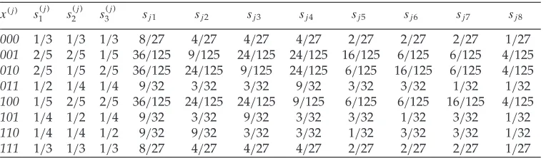
Table 1: The transition probabilities for the selection operator.

x(j) _s(j) 1 s

(j) 2 s

(j)

3 sj1 sj2 sj3 sj4 sj5 sj6 sj7 sj8

000 1/3 1/3 1/3 8/27 4/27 4/27 4/27 2/27 2/27 2/27 1/27

001 2/5 2/5 1/5 36/125 9/125 24/125 24/125 16/125 6/125 6/125 4/125

010 2/5 1/5 2/5 36/125 24/125 9/125 24/125 6/125 16/125 6/125 4/125

011 1/2 1/4 1/4 9/32 3/32 3/32 9/32 3/32 3/32 1/32 1/32

100 1/5 2/5 2/5 36/125 24/125 24/125 9/125 6/125 6/125 16/125 4/125

101 1/4 1/2 1/4 9/32 3/32 9/32 3/32 3/32 1/32 3/32 1/32

110 1/4 1/4 1/2 9/32 9/32 3/32 3/32 1/32 3/32 3/32 1/32

111 1/3 1/3 1/3 8/27 4/27 4/27 4/27 2/27 2/27 2/27 1/27

We use the local fitness from Equation (5). Also, in this paper, we will take

S_norm(j) =m

k=1(1−g(xk|x

(j)_{)), ∀i∈ {1, . . . , m}, x}(j)_{∈S (9)}

and thus3i₌1s (j)

i =1 for allj. Hence, in our simple running example, independently of the statej, on average, a single bit will be selected for conversion to a #. One can say that together the analysis and selection believe a 0 is incorrect and so will often convert one of the 0s to a # but they cannot be certain and so will also sometimes select a 1 for conversion to #.

Computation of the transition matrix is straightforward; for example,S_norm000 =3∗ (1−1/3)=2, givings₀000=(1−1/3)/2=1/3. Since the bits are selected independently, for any solutionx(j), the various transition probabilities are simply

sj1 ≡pS

Xn+1 =(x1, x2, x3)(j)|Xn=(x1, x2, x3)(j)

=1−s₁(j) 1−s₂(j) 1−s₃(j) ,

sj2 ≡pS

Xn+1 =(x1, x2,#)(j)|Xn=(x1, x2, x3)(j)

=1−s₁(j) 1−s₂(j) s₃(j),

sj3 ≡pS

Xn+1 =(x1,#, x3)(j)|Xn=(x1, x2, x3)(j)

=1−s₁(j) s₂(j)1−s₃(j) ,

sj4 ≡pS

Xn+1 =(#, x2, x3)(j)|Xn=(x1, x2, x3)(j)

=s₁(j)1−s₂(j) 1−s₃(j) ,

sj5 ≡pS

Xn+1 =(#,#, x3)(j)|Xn=(x1, x2, x3)(j)

=s₁(j)s₂(j)1−s₃(j) ,

sj6 ≡pS

Xn+1 =(#, x2,#)(j)|Xn=(x1, x2, x3)(j)

=s₁(j)1−s₂(j) s₃(j),

sj7 ≡pS

Xn+1 =(x1,#,#)(j)|Xn=(x1, x2, x3)(j)

=1−s₁(j) s₂(j)s₃(j),

sj8 ≡pS

Xn+1 =(#,#,#)(j)|Xn=(x1, x2, x3)(j)

=s₁(j)s₂(j)s(₃j).

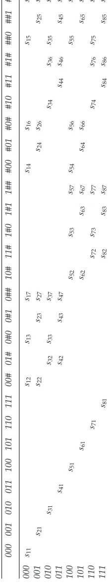
Table 1 shows the detailed values of all non-zero transition probabilities for the selection operator. Note that, except for the symmetric states 000 and 111, a 0 bit is precisely twice as likely to be selected as a 1. Table 2 shows the structure of its associated transition matrixS8×27.

3.5 The Mutation Operator

The mutation operator is a map from spaceS#to itself that, independently for each part of the solution, will randomly convert a non-# to a # (for reinstantiation by the later construction operator). It is similar to the selection operator, except that the mutations do not use any analysis of the solution but are purely random, and also the formalism has to allow the possibility that the element is already a # due to the preceding selection step.

The probabilities that any non-# componentx_i from tuplex=(x₁, . . . , x_m) is con-verted to a # is taken to be a mutation probabilityq_M∈[0,1]. Note that, for simplicity, we take the mutation probability to be the same for all components, i, but this could easily be extended if desired. It is usually taken to be a non-zero so as to increase di-versification, and to be a constant; though it could, if desired, be allowed to change on each iteration.

Letp_M(Xn+1=x|Xn=x) be the conditional probability that tuplex=(x₁, . . . , xm) is generated from tuplex=(x₁, . . . , x_m) by the mutation operator, then:

p_M(Xn+1 =x|Xn=x)=

0, iff ∃i∈ {1, . . . , m}, x_i=x_iandx_i= #; m

i=1(qMD(x

i,xi)(1−q_M)1-D(x

i,xi)₎1-λi_{, otherwise,} (10)

where the constants

D(x_i, x_i)=

1, ifx_i= # andx_i= #;

0, ifx_i= # andx_i= #, (11)

λi =

1, ifx_i=x_i= #;

0, otherwise (12)

simply capture that the mutation is only permitted to change a non-# to a #.

EXAMPLE2: State transitions by a mutation operator.

Returning to the running example, and takingq_M=1/10, the resulting transition matrixM27×27for the mutation step, is given in explicit detail in Table 3.

3.6 The Construction Operator

The last operator, construction, is a linear map from spaceS#back to the original spaceS. Letp_C(Xn+1 =x|Xn=x) be the conditional probability that tuplex=(x₁, . . . , xm) is generated from tuplex=(x₁, . . . , x_m) by the construction operator. LetN(x) be the set of all possible destination states that can be constructed from intermediate statex. Clearly,|N(x)| =nl#_{, wherel}

#is the number of # inx.

diversification in the search. There are many possibilities for how to do this probabilistic bias, but here we initially take:

p_C(Xn₊1=x|Xn=x)= ⎧ ⎪ ⎨ ⎪ ⎩

0, if∃i∈ {1, . . . , m}, x_i=# andx_i=x_i; 1, if∀i∈ {1, . . . , m}, x_i=x_i;

f(x)

X∈N(x)f(X), otherwise.

(13)

The first two cases of Equation (13) are automatic constraints in that they merely say that the constructor can only assign values to unassigned, #, variables. We will assume thatf(x)>0,∀x ∈S, which, if needed, is easily achieved by adding a constant to f. This is also the reason for the+1 in Equation (4).

A method to implement this would be to enumerate the elements of |N(x)| and then perform a tournament style selection weighted by fitness. However,|N(x)| =nl#_,

and so increases exponentially withl_#, and would quickly become impractical for larger values ofl_#.

Hence, to reduce the amount of computation required during the construction step, we introduce a threshold parameter t, and if the number of #s exceeds t, a simple unbiased random construction is performed in which all the neighboring states have an equal probability to be reached. This gives a revised version of Equation (13), and the constructor that we use is defined by

p_C(Xn₊1=x|Xn=x)= ⎧ ⎪ ⎪ ⎪ ⎪ ⎨ ⎪ ⎪ ⎪ ⎪ ⎩

0, if∃i∈ {1, . . . , m}, x_i=# andx_i=x_i; 1, if∀i∈ {1, . . . , m}, x_i =x_i;

1/nl_{#, ifl}

#> t;

f(x)

X∈N(x)f(X)

, otherwise.

(14)

Note thatt =0 corresponds to a random constructor, andt =mto Equation (13). We will useC Ltto refer to different choices fort.

Equation (14) is a specific choice for a constructor and the primary choice that defines the algorithm to be ESWO-II rather than a general ESWO. Recall that the intent of the randomized constructive method is to have some variability but still to favor the construction of fitter solutions. However, in order to be able to perform the analysis, we still wanted something with a declarative definition, rather than only being defined using some heuristic construction method.

Note that the constructor has no memory of the state of the prior state of a # before it was unassigned. The selection or mutation that converts an element to a # does not necessarily ultimately force it to change. This makes it different from standard local search in which a move is intrinsically to a different state; the possibility to keep the same state presumably plays a similar role as the rejection of moves under a metaheuristic such as simulated annealing.

EXAMPLE3: State transitions by a simple construction operator.

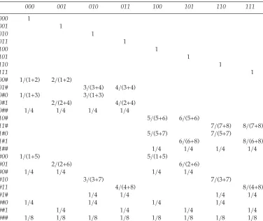
Table 4: The transition matrix of construction (with blank entries being zero probabilities).

000 001 010 011 100 101 110 111

000 1

001 1

010 1

011 1

100 1

101 1

110 1

111 1

00# 1/(1+2) 2/(1+2)

01# 3/(3+4) 4/(3+4)

0#0 1/(1+3) 3/(1+3)

0#1 2/(2+4) 4/(2+4)

0## 1/4 1/4 1/4 1/4

10# 5/(5+6) 6/(5+6)

11# 7/(7+8) 8/(7+8)

1#0 5/(5+7) 7/(5+7)

1#1 6/(6+8) 8/(6+8)

1## 1/4 1/4 1/4 1/4

#00 1/(1+5) 5/(1+5)

#01 2/(2+6) 6/(2+6)

#0# 1/4 1/4 1/4 1/4

#10 3/(3+7) 7/(3+7)

#11 4/(4+8) 8/(4+8)

#1# 1/4 1/4 1/4 1/4

##0 1/4 1/4 1/4 1/4

##1 1/4 1/4 1/4 1/4

### 1/8 1/8 1/8 1/8 1/8 1/8 1/8 1/8

probability, regardless of its global fitness value. Recall from Equation (4) that the global fitness function is simply one plus the decimal value of a binary vector when it is regarded as a binary number.

Table 4 shows the probability values of transition matrixC27×8after the construction step.

4

Markov Chain Model for ESWO-II

We first give a basic definition that is a natural extension to the standard stochastic matrix. It arises because of the way that the search moves through intermediate states and spaces of different dimensions.

DEFINITION7: A matrixT=[tij]m×nis row-stochastic ifTis not necessarily a square matrix

(i.e., m does not necessarily equaln), but still satisfies: tij ∈[0,1] and

n

j=1tij =1 for all

i= {1, . . . , m}.

LEMMA1: LetSbe anm×nrow-stochastic matrix,Mann×nstochastic matrix, andCan

n×mrow-stochastic matrix. Then the productS·M·Cis a stochastic matrix.

Assume that a solution consists of mvariablesxi,i∈ {1, . . . , m}, and eachxi may take one of the n values, that is, xi ∈ {j1, . . . , jn}. The selection operator carries out a linear map from space S of cardinalitynm to spaceS of cardinality (n+1)m_{, with} a transition matrix S=[sij]nm_×(n+1)m defined by Equations (6), (7), and (8). Next, the

mutation operator carries out a linear map from spaceSof cardinality (n+1)m_{to itself,} with transition matrix M=[mij](n+1)m_×(n+1)m defined by Equations (8), (9), and (10).

Finally, the construction operator carries out a linear map from spaceSof cardinality (n+1)m _{back to the original spaceS of cardinalityn}m_{, with a transition matrixC=} [cij](n+1)m×nm defined by Equation (13) or Equation (14). By Lemma 1, we have the

following statement immediately.

LEMMA2: All state transitions of the ESWO-II algorithm with component selection, fixed

rate mutation and solution construction are probabilistic (in the sense of it being possible to model with a Markov stochastic process).

The three operators of selection, mutation, and construction work as a whole to carry out a linear transformation from state space S to itself, by an overall transition matrix

P which is the product of three intermediate-transformation matrices corresponding to the individual operators. Note that the Markov chain of the ESWO-II algorithm is homogeneous as none of the matrices depend on time. Hence, many standard theorems of Markov analysis apply directly.

In theoretical studies of genetic algorithms, the most well-known class of evolution-ary algorithms, an overall transition matrix is also achieved through the multiplication of matrices corresponding to the transition operators of selection, crossover, and mu-tation (Rudolph, 1994; Agapie, 1998). Although it has the same names for two of the operators, the state transition process of our proposed ESWO-II algorithm is quite dif-ferent from that of genetic algorithms. Each of the genetic algorithms’ operators is a map within the same problem space (i.e., endomorphism), while this is not the case for the ESWO-II algorithm.

THEOREM2: If the mutation probability is non-zero,q_M>0, then the ESWO-II algorithm using the constructor of Equation (13) or (14) visits the global optimal set with probability one.

PROOF(SHORT): As long as the mutation rate is strictly positive,q_M>0, then on any iteration there is a strictly positive probability that all elements will be unassigned and converted to a #. Also, by construction, there is a strictly positive probability of generating any optimal solution. Hence, by going through the state of purely #s there is a non-zero chance of reaching an optimal state in a single iteration.

Note that the theorem also applies ifq_M=0 as long as the selection probability is non-zero. The following longer proof sketch is given in fuller detail simply because it is useful for actual calculations for the tables given later.

PROOF(DETAILED): To simplify the presentation, we defineα=nmandβ=(n+1)m−

The selection transition matrix can be partitioned into the following two block matrices,S=Dα Sα_×β

where diagonal matrixD, with elementsdk, corresponds to the situations of no components being selected. It is convenient to writedkl=dkifk=l anddkl=0 ifk=l. The rectangular matrixS’ corresponds to the situations of at least one of the components being selected.

The transition matrix M of mutation can be partitioned into the following four

block matrices M=

tInm M_α×β

0β×α Mβ×β

, wheret =(1−q_M)nm

where q_M is the mutation rate. Diagonal matrixtIand rectangular matrixMare based on the condition that no component has been previously selected: tIcorresponds to the situation of no com-ponents being mutated again, whileMcorresponds to the situation of at least one of the components being mutated. Zero matrix 0and upper triangular matrixM(with all diagonal entries being non-zero) are based on the condition that at least one of the components has been previously selected:0means that no destination state is reachable from the intermediate states, andMcorresponds to the situations of components being further mutated from the intermediate states.

The transition matrixCof construction can be partitioned into the following two

block matrices C=

Iα

Cβ×α

, where identity matrixImeans that a state remains the

same if no components of it have been selected or mutated, and matrixCdenotes the transition probabilities from intermediate states to destination states by construction.

The overall transition matrix is then

P=S·M·C=tDα+DαMα×βCβ×α+Sα×βMβ×βCβ×α

=tDα+(D·M·C)α×α+(S·M·C)α×α

. (15)

Writing each term in full then gives

tD=

⎡ ⎢ ⎣

t d₁ · · · 0 .. . . .. ... 0 · · ·t dα

⎤ ⎥ ⎦

D·M·C=

⎡ ⎢ ⎢ ⎢ ⎢ ⎢ ⎢ ⎣ d₁ β

i=1

m_1ic_i1 · · · d₁ β

i=1

m_1ic_iα ..

. . .. ...

dα β

i₌1

m_αic_i1 · · ·dα β

i₌1

m_αic_iα ⎤ ⎥ ⎥ ⎥ ⎥ ⎥ ⎥ ⎦

S·M·C=

⎡ ⎢ ⎢ ⎢ ⎢ ⎢ ⎢ ⎣ β

i=1

β

j=1

s_1jm_{j i}c_i1 · · · β

i=1

β

j=1

s_1jm_{j i}c_iα ..

. . .. ...

β

i=1

β

j=1

s_αj m_{j i}c_i1 · · · β

i=1

β

j=1

Hence, finally, the transition matrixPis ⎡ ⎢ ⎢ ⎢ ⎢ ⎢ ⎢ ⎣

t d₁+d₁ β

i=1

m_1ic_i1+ β

i=1

β

j=1

s_1jm_{j i}c_i1 · · · d₁ β

i=1

m_1ic_iα+ β

i=1

β

j=1

s_1jm_{j i}c_iα ..

. . .. ...

dα β

i=1

m_αic_i1+ β

i=1

β

j=1

s_αj m_{j i}c_i1 · · · t dα+dα β

i=1

m_αic_iα+ β

i=1

β

j=1

s_αjm_{j i}c_iα ⎤ ⎥ ⎥ ⎥ ⎥ ⎥ ⎥ ⎦ (16)

or more compactly

Pkl =t dkl+dk β

i=1

m_kic_il+ β

i=1

β

j=1

s_kj m_{j i}c_il. (17)

Note that all the terms are nonnegative, hence, for allk, l

Pkl ≥dk β

i=1

m_kic_il

≥dkmkβcβl

=dk (qM)m

nm >0.

Note that the state indexed byβ is taken to be the one with purely #s. This suffices to show that the matrix is regular (and ergodic) for the typical case thatdk>0,qM>0 and c_βl>0, meaning that for every element, even if it is not selected, it may be chosen for mutation, and has a probability of reaching any state. Hence, the ESWO-II algorithm visits a global optimum after a finite (possibly very large) number of transition steps,

regardless of the starting states, with probability one.

If, furthermore, we assume that the various operators are constants, for example, the mutation probability is constant and non-zero, then it follows by Theorem 1 that there exists a unique stationary probability distributionπ=(π₁, . . . , π_|S|), andπj >0 for 1≤j ≤ |S|, and so again the optima have non-zero probability. However, of course, it does not converge in the sense of all of the probability lying only on optimal solutions— because all states and not just optima have some non-zero probability.

Naturally, in real world applications, a stochastic algorithm such as ESWO-II always keeps the best solution found over time. Then clearly:

COROLLARY 1: The ESWO-II algorithm, maintaining the best solution found over time,

converges to the global optimum.

Hence, by the extension of Theorem 1 to a reducible Markov chain, the probability of remaining in the set of non-closed states converges to zero.

5

Discussion of Results on Stationary Distribution

LEMMA3: Consider a finite Markov chain with a regular transition matrixP. If matrixPis

symmetric then the stationary probabilities{πi, i∈S}are equally distributed, with a value of

1/|S|, on stateifor alli∈S.

PROOF: AsPis stochastic, we have_i∈Spj i=1,∀j ∈S. IfPis symmetric, thenpij = pj i,∀i, j∈S⇒

i∈Spij =1,∀j ∈S⇒ _|S1_| =

i∈S _|1S|pij,∀j ∈S. The vectorπ with a value of 1/|S| on each state is a stationary distribution of P, since the equilibrium equations and the normalizing condition as given in Definition 2 are all satisfied. Fur-thermore, by Theorem 1, for any regular transition matrixP, the stationary probability distributionπ =(π1, . . . , π|S|) is unique. Hence, we can conclude that such a vectorπ is the only stationary distribution ifPis a symmetric regular matrix.

LEMMA4: For a state ofa ∈S and an intermediate stateb∈S, one step of transition by

selection and mutation cannot changeatob, if and only if one step of transition by construction

cannot changebtoa.

REMARK: This is “by construction” because a selection with mutation can only change

a complete assignment to a partial assignment by changing entries to a # without changing any entries otherwise. The construction can only affect # entries. In ESWO-II, any such allowed changes also have some probability of happening.

Next, we investigate the conditions on which the stationary probabilities are equally distributed. The following theorem will aid our later discussion.

THEOREM 3: For an ESWO-II algorithm with a randomized selection and a randomized

construction, irrespective of the rate of mutation (as long as it is non-zero), the stationary

probabilities{πi, i∈S}are equally distributed on each statei.

By a randomized selector, we just mean one that has no attempt to bias toward any one solution, and so for exampleg(xi1|x(

j)_)=g(x

i2|x(

j)_{) holds for allx}

i1andxi2; we will

denote this byS rand. Similarly, a purely random constructor,CL0, is, for example, also given by the caset=0 of Equation (14), in which all legal transitions are equally likely. PROOF SKETCH: Since the randomized selection and construction treat all states inS equally, then there is no bias toward any one state and so the only sensible distribution is uniform. A direct proof is possible using Equation (17), but is omitted as it is long

and not informative.

EXAMPLE4: Transition matrices by randomized selection and a randomized construction.

In addition to the previous examples wheref(x)=4x₁+2x₂+x₃+1, we imple-ment various combinations of different types of operators as follows:

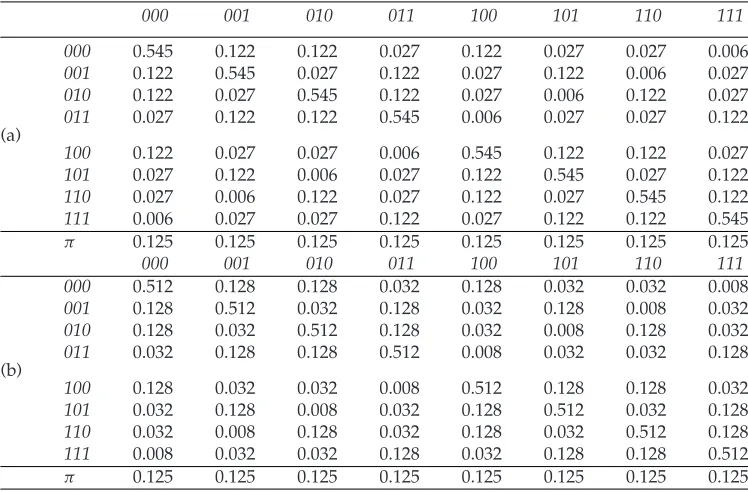
Table 5: Transition matrices: (a) Srand×M05×Crand, and (b)Srand×M10×

C rand.

000 001 010 011 100 101 110 111

000 0.545 0.122 0.122 0.027 0.122 0.027 0.027 0.006

001 0.122 0.545 0.027 0.122 0.027 0.122 0.006 0.027

010 0.122 0.027 0.545 0.122 0.027 0.006 0.122 0.027

011 0.027 0.122 0.122 0.545 0.006 0.027 0.027 0.122

(a)

100 0.122 0.027 0.027 0.006 0.545 0.122 0.122 0.027

101 0.027 0.122 0.006 0.027 0.122 0.545 0.027 0.122

110 0.027 0.006 0.122 0.027 0.122 0.027 0.545 0.122

111 0.006 0.027 0.027 0.122 0.027 0.122 0.122 0.545

π 0.125 0.125 0.125 0.125 0.125 0.125 0.125 0.125

000 001 010 011 100 101 110 111

000 0.512 0.128 0.128 0.032 0.128 0.032 0.032 0.008

001 0.128 0.512 0.032 0.128 0.032 0.128 0.008 0.032

010 0.128 0.032 0.512 0.128 0.032 0.008 0.128 0.032

011 0.032 0.128 0.128 0.512 0.008 0.032 0.032 0.128

(b)

100 0.128 0.032 0.032 0.008 0.512 0.128 0.128 0.032

101 0.032 0.128 0.008 0.032 0.128 0.512 0.032 0.128

110 0.032 0.008 0.128 0.032 0.128 0.032 0.512 0.128

111 0.008 0.032 0.032 0.128 0.032 0.128 0.128 0.512

π 0.125 0.125 0.125 0.125 0.125 0.125 0.125 0.125

Equation (5), andS reve denotes the one that defines its component fitness as 1−g(xi|x(j)) (i.e., the reverse of operatorS).

• For the mutation operator,M05 denotes the case ofq_M=0.05 in Equation (10),

M10 the case ofqM=0.10, andM20 the case ofqM=0.20.

• For the construction operator,Crand denotes the randomized one as introduced in Theorem 3,CL1 denotes the case oft=1 in Equation (17), andC L2 denotes the case oft=2.

Table 5 shows two transition matrices of using randomized operators or selection and construction, with different mutation operators (i.e.,M 05 andM 10). The com-putations are standard and are implemented using MATLAB. We can see that the two matrices are different due to differentq_Msettings, but they are all symmetric matrices and thus have the same equally distributed stationary distribution vectorsπ.

As we have seen explicitly, when the steps of selection and construction are all randomized then the process is ergodic and furthermore all states are equally likely. Naturally, the final distribution is not always uniform, and we have the following statement.

COROLLARY2: For the ESWO-II algorithm, the stationary probability distribution{πi, i∈S} on individual states is affected by the strategies of selection, mutation, and construction.

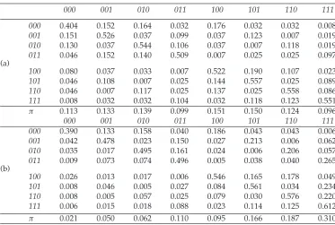
Table 6: Transition matrices: (a)S reve×M10×CL1, and (b)S×M05×CL2.

000 001 010 011 100 101 110 111

000 0.404 0.152 0.164 0.032 0.176 0.032 0.032 0.008

001 0.151 0.526 0.037 0.099 0.037 0.123 0.007 0.019

010 0.130 0.037 0.544 0.106 0.037 0.007 0.118 0.019

011 0.046 0.152 0.140 0.509 0.007 0.025 0.025 0.097

(a)

100 0.080 0.037 0.033 0.007 0.522 0.190 0.107 0.023

101 0.046 0.108 0.007 0.025 0.144 0.557 0.025 0.089

110 0.046 0.007 0.117 0.025 0.137 0.025 0.558 0.086

111 0.008 0.032 0.032 0.104 0.032 0.118 0.123 0.551

π 0.113 0.133 0.139 0.099 0.151 0.150 0.124 0.096

000 001 010 011 100 101 110 111

000 0.390 0.133 0.158 0.040 0.186 0.043 0.043 0.006

001 0.042 0.478 0.023 0.150 0.027 0.213 0.006 0.062

010 0.035 0.017 0.495 0.161 0.024 0.006 0.206 0.057

011 0.009 0.073 0.074 0.496 0.005 0.038 0.040 0.265

(b)

100 0.026 0.013 0.017 0.006 0.546 0.165 0.178 0.049

101 0.008 0.046 0.005 0.027 0.084 0.561 0.034 0.234

110 0.008 0.005 0.057 0.025 0.079 0.030 0.576 0.220

111 0.006 0.015 0.018 0.088 0.023 0.114 0.125 0.612

π 0.021 0.050 0.062 0.110 0.095 0.166 0.187 0.310

best solution found over time, a stationary probability close to one could be distributed on the optimal solution of the given problem instance.

EXAMPLE5: Stationary probability distributions caused by different ESWO-II operators.

Table 6 shows two transition matrices of using different combinations of selection, mutation, and construction operators (i.e., S reve ×M 10× CL1 andS ×M 05×

C L2). We can see that the two matrices are not symmetric and are very different. In particular, their stationary distribution vectors π differ significantly, which is in line with Corollary 2.

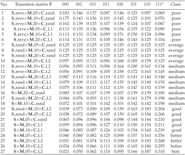
Table 7: Stationary distributions: full strategy combinations (* denotes optimal solutions).

No. Transition matrixP 000 001 010 011 100 101 110 111* Class 1 Sreve×M05×Crand 0.183 0.146 0.137 0.097 0.146 0.125 0.097 0.069 poor 2 Sreve×M10×Crand 0.175 0.143 0.136 0.101 0.143 0.125 0.101 0.076 poor 3 Sreve×M20×Crand 0.162 0.139 0.133 0.107 0.139 0.124 0.107 0.087 poor 4 Sreve×M 05×CL1 0.113 0.135 0.136 0.096 0.154 0.155 0.122 0.090 poor 5 Sreve×M 10×CL1 0.113 0.133 0.134 0.099 0.151 0.150 0.124 0.096 poor 6 Sreve×M 20×CL1 0.114 0.131 0.131 0.105 0.146 0.143 0.125 0.104 poor 7 Srand×M05×Crand 0.125 0.125 0.125 0.125 0.125 0.125 0.125 0.125 average 8 Srand×M10×Crand 0.125 0.125 0.125 0.125 0.125 0.125 0.125 0.125 average 9 Srand×M20×Crand 0.125 0.125 0.125 0.125 0.125 0.125 0.125 0.125 average 10 Sreve×M05×CL2 0.057 0.095 0.113 0.096 0.168 0.185 0.159 0.125 average 11 Sreve×M10×CL2 0.056 0.093 0.111 0.096 0.164 0.180 0.161 0.134 medium 12 Sreve×M20×CL2 0.056 0.091 0.109 0.105 0.158 0.172 0.163 0.145 medium 13 Srand×M20×CL1 0.087 0.113 0.116 0.119 0.133 0.141 0.144 0.148 medium 14 Srand×M10×CL1 0.079 0.109 0.113 0.117 0.135 0.145 0.149 0.155 medium 15 Srand×M05×CL1 0.075 0.106 0.111 0.112 0.135 0.147 0.152 0.159 medium 16 S×M20×Crand 0.083 0.107 0.107 0.139 0.107 0.139 0.139 0.180 medium 17 Srand×M20×CL2 0.044 0.076 0.093 0.111 0.138 0.161 0.179 0.198 medium 18 S×M10×Crand 0.072 0.101 0.101 0.142 0.101 0.142 0.142 0.198 medium 19 Srand×M10×CL2 0.039 0.073 0.090 0.109 0.139 0.163 0.183 0.204 good 20 Srand×M05×CL2 0.038 0.072 0.089 0.107 0.139 0.165 0.184 0.206 good 21 S×M05×Crand 0.065 0.096 0.096 0.144 0.098 0.144 0.144 0.210 good 22 S×M20×CL1 0.059 0.094 0.096 0.127 0.110 0.150 0.154 0.211 good 23 S×M10×CL1 0.046 0.085 0.087 0.126 0.103 0.154 0.160 0.239 good 24 S×M05×CL1 0.040 0.080 0.082 0.125 0.098 0.157 0.163 0.256 better 25 S×M20×CL2 0.031 0.061 0.074 0.113 0.108 0.163 0.183 0.268 better 26 S×M10×CL2 0.024 0.054 0.066 0.111 0.100 0.165 0.186 0.295 better 27 S×M05×CL2 0.021 0.050 0.062 0.110 0.095 0.166 0.187 0.310 best

moves are accepted. In fact, this supports our original motivations that understanding ESWO will need a good understanding of the separate stages, and their interaction.

Next, we use the following example to verify experimentally that certain strategies do make the optimal solution have higherπivalues.

EXAMPLE6: Key factors affecting the stationary probability distribution.

Consider further the previous examples wheref(x(j)_)=4x

1+2x2+x3+1 is used. Then the optimal solution of the toy problem is 111, with fitness values increasing as we move to the right in the tables. Table 7 shows the stationary distribution vectorsπof transition matrices obtained by a full combination of selection, mutation, and construc-tion strategies. The staconstruc-tionary probabilities of the optimal soluconstruc-tion are displayed in the second to last column in ascending order, and indicative class values (i.e., poor, average, medium, good, better, or best) are displayed as a rough guide in the last column.

π₍₁₁₁₎are no higher than average unless aCL2 is jointly used, which makesπ₍₁₁₁₎a little bit higher than average on two cases (but still on the bottom of the medium list). Fur-thermore, as long as anSrand or aCrand operator (but not both) is used,π₍₁₁₁₎values fall into the class medium or the bottom of class good. The interesting thing is that a joint use ofSandCL2 achieves the top threeπ₍₁₁₁₎values, and in particular, the smallest mutation rate (i.e.,M 05) generates the highest value. The above observations suggest that, to achieve the best system performance, selection may play the most important role, construction the second, and mutation the third.

Observe that line 21 of Table 7 shows that a biased selector in itself is enough to cause a bias toward the optimal, even with an unbiased (random) constructor. This makes sense because if we count 0 as a flaw, then even with a random constructor, it has a 50% chance of being converted to 1, and this will be an improvement. Arguably, overall, this makes ESWO-II rather more similar to standard iterative repair (e.g., see Minton et al., 1992) than to SWO.

6

Conclusions

In this paper, we have developed a formal framework for extending ESWO to ESWO-II by revising the ESWO’s construction step to enable probabilistic choices among dif-ferent possible destination states in a flexible way. Firstly, we focused on ESWO-II’s convergence behavior. By a finite Markov chain analysis, we confirm that (unsurpris-ingly) although the global optimum is reachable after finite transitions with probability one, convergence to the global optimum is not. Also, after studying its transition matrix, we find that for the ESWO-II algorithm, the stationary distribution on individual states is not only affected but also controllable by the choices of the selection function, the mutation rate, and the construction function. The last result suggests that, by a proper implementation of the ESWO-II algorithm, even without using the strategy of saving the previous best solutions, if desired, the algorithm could be controlled so as to con-verge to an optimal solution (in the same sense as SA does when the temperature is cooled correctly).

Possibly, though further study is required, controlling such concentration around the optima will mean that an optimal solution will be reached much earlier than other solutions during the progress of the algorithm. Note that in simulated annealing, very small temperatures are best concentrated around optima, but are not the best for re-ducing the time to reach the optima, because the high concentration actually causes a loss of diversity in the search and so hitting times increase. With SA, this means that temperatures need to be carefully controlled. It is far from clear whether or not the same issues also apply to ESWO-II, and such an analysis would be a major goal of future work.

Finally, in our empirical studies, we considered time-independent operators. How-ever, this is not forced; for example, for the mutation operator, we could use a (slowly)-varying mutation rate, which makes the corresponding Markov chain (quasi-) inhomogeneous. These advanced strategies will result in different Markov modeling and convergence behaviors, and we intend to investigate them in future.

Acknowledgments

The research described in this paper was funded by the Engineering and Physical Sciences Research Council (EPSRC), under grants EP/D061571/1 and EP/F033214/1.

References

Agapie, A. (1998). Genetic algorithms: Minimal conditions for convergence. Artificial Evolution, Lecture Notes in Computer Science, 1363:181–193.

Aickelin, U., Burke, E. K., and Li, J. (2009). An evolutionary squeaky wheel optimisation approach to personnel scheduling.IEEE Transactions on Evolutionary Computation, 13:433–443.

Aickelin, U., and Li, J. (2007). An estimation of distribution algorithm for nurse scheduling.

Annals of Operations Research, 155:289–309.

Barbulescu, L., Watson, J. P., Whitley, L., and Howe, A. E. (2004). Scheduling space–ground communications for the air force satellite control network. Journal of Scheduling, 27:7–34.

Burke, E. K., Hyde, M., and Kendall, G. (2010). A squeaky wheel optimisation methodology for two dimensional strip packing.Computers & Operations Research, 14:942–958.

Burke, E. K., and Newall, J. P. (2004). Solving examination timetabling problems through adap-tation of heuristic orderings.Annals of Operations Research, 129:107–134.

Dorigo, M., Maniezzo, V., and Colorni, A. (1996). Ant system: Optimization by a colony of cooperating agents.IEEE Transactions on Systems, Man, and Cybernetics, Part B, 26:29–41.

Feng, G., and Lau, H. (2008). Efficient algorithms for machine scheduling problems with earliness and tardiness penalties.Annals of Operations Research, 159:83–95.

Feo, A., and Resende, M. G. C. (1989). A probabilistic heuristic for a computationally difficult set covering problem.Operations Research Letters, 8:67–71.

Fu, Z., Li, Y., Lim, A., and Rodrigues, B. (2007). Port space allocation with a time dimension.

Journal of the Operational Research Society, 58:797–807.

Gendreau, M., and Potvin, J. Y. (2010). Handbook of meta-heuristics, 2nd ed. Berlin: Springer.

Ginsberg, M. L. (2001). Gib: Imperfect information in a computationally challenging game.Journal of Artificial Intelligence Research, 14:303–358.

Glover, F. (1989). Tabu search, Part I.ORSA Journal on Computing, 1:190–206.

Goldberg, D. (1989). Genetic algorithms in search, optimization and machine learning. Reading, MA: Addison-Wesley.

Hansen, P., and Mladenovi´c, N. (1999). Variable neighbourhood search: Principles and applica-tions.European Journal of Operational Research, 130:449–467.

Joslin, D., and Clements, D. P. (1999). Squeaky wheel optimization.Journal of Artificial Intelligence Research, 10:353–373.

Kirkpatrick, S., Gelatt, C., and Vecchi, M. (1983). Optimization by simulated annealing. Science, 220:671–680.

Koralov, L. B., and Sinai, Y. G. (2007).Theory of probability and random processes. Berlin: Springer.

Larra ˜naga, P., and Lozano, J. A. (2002). Estimation of distribution algorithms: A new tool for evolu-tionary computation. Dordrecht, The Netherlands: Kluwer Academic Publishers.

Li, J., and Kwan, R. S. K. (2003). A fuzzy genetic algorithm for driver scheduling.European Journal of Operational Research, 147:334–344.

Lim, A., Rodrigues, B., Xiao, F., and Zhu, Y. (2004). Crane scheduling with spatial constraints.

Naval Research Logistics, 51:386–406.

Malaguti, E., and Toth, P. (2008). An evolutionary approach for bandwidth multicoloring prob-lems.European Journal of Operational Research, 189:638–651.

Michiels, W., Aarts, E., and Korst, E. J. (2007).Theoretical aspects of local search. Berlin: Springer.

Minton, S., Johnston, M. D., Philips, A. B., and Laird, P. (1992). Minimizing conflicts: A heuris-tic repair method for constraint satisfaction and scheduling problems.Artificial Intelligence Journal, 58:161–205.

Papadimitriou, C. H., and Steiglitz, K. (1982).Combinatorial optimization—Algorithms and complex-ity. New York: Dover.

Rudolph, G. (1994). Convergence analysis of canonical genetic algorithms. IEEE Transactions on Neural Networks, 5:96–101.