1
A two-stage stochastic mixed-integer program modelling and
hybrid solution approach to portfolio selection problems
Fang He, Rong Qu
The Automated Scheduling, Optimisation and Planning (ASAP) Group, School of Computer Science The University of Nottingham, Nottingham, NG8 1BB, UK
{[email protected], [email protected] }
Abstract
In this paper, we investigate a multi-period portfolio selection problem with a comprehensive set of real-world trading constraints as well as market random uncertainty in terms of asset prices. We formulate the problem into a two-stage stochastic mixed-integer program (SMIP) with recourse. The set of constraints is modelled as mixed-integer program, while a set of decision variables to rebalance the portfolio in multiple periods is explicitly introduced as the recourse variables in the second stage of stochastic program. Although the combination of stochastic program and mixed-integer program leads to computational challenges in finding solutions to the problem, the proposed SMIP model provides an insightful and flexible description of the problem. The model also enables the investors the make decisions subject to real-world trading constraints and market uncertainty.
To deal with the computational difficulty of the proposed model, a simplification and hybrid solution method is applied in the paper. The simplification method aims to eliminate the difficult constraints in the model, resulting into easier sub-problems compared to the original one. The hybrid method is developed to integrate local search with Branch-and-Bound (B&B) to solve the problem heuristically. We present computational results of the hybrid approach to analyse the performance of the proposed method. The results illustrate that the hybrid method can generate good solutions in a reasonable amount of computational time. We also compare the obtained portfolio values against an index value to illustrate the performance and strengths of the proposed SMIP model. Implications of the model and future work are also discussed.
Key words: Stochastic programming; hybrid algorithm; Branch-and-Bound; local search; portfolio selection problems
1. Introduction
The essence of portfolio selection problem (PSP) can be described as finding a combination of assets that best satisfies an investor’s needs. The theory of PSP was developed by Harry Markowitz firstly in the 1950’s. In his work, the PSP was formulated as the mean–variance (MV) model (Markowitz 1952), a quadratic optimisation model. The basic MV model selects the composition of assets which either achieves a predetermined level of expected return while minimizing the risk, or achieves the maximum expected return within a predefined level of risk.
2
considered into the basic MV model, the problem is recognized to be NP-complete (Bienstock 1996, Mansini and Speranza 1999).
Along with the trading constraints, another important factor faced by the investors to make a proper investment decision is the market uncertainty. However, in the classic MV model and other models of PSP (Chang, Meade et al. 2000, Kellerer, Mansini et al. 2000, Crama and Schyns 2003, Konno and Yamamoto 2005, Mansini and Speranza 2005), the expected return and covariance between assets are usually based directly on historical data. These models do not account for the uncertainties of the market.
Financial markets are unpredictable and decision should be made with the consideration of market conditions (Ji, Zhu et al. 2005, Baldacci, Boschetti et al. 2009). Moreover, investors apply flexible portfolio management strategies by rebalancing portfolios periodically in response to new uncertain market conditions (i.e. changing perceptions regarding the random asset price). Random uncertainties of market, i.e., in terms of asset prices and currency exchange rates etc. are main factors of market. Several non-probabilistic uncertainty factors such as vagueness and ambiguity are investigated mainly by fuzzy techniques (Gupta, Mehlawat et al. 2010, Gupta, Inuiguchi et al. 2013, Li and Xu 2013). In this paper we focus on random uncertainty of the market, i.e., in term of asset prices.
Stochastic programming becomes an increasingly popular technique to model decision making under random uncertainty. It is able to model uncertainties in a flexible way and impose real-world constraints relatively easily (King and Wallace 2012). It uses information in the future to make current decisions. Higle and Wallace (Higle and Wallace 2003) investigate the uncertainty factors in general stochastic problems. Generally speaking, taking into account of uncertainty helps to improve decision making.
Stochastic programming has been applied to describe a variety of portfolio optimization problems. Models for asset-liability and risk management have been proposed in (Mulvey and Vladimirou 1992), (Topaloglou, Vladimirou et al. 2008, Stoyan and Kwon 2011). New approaches based on stochastic programming for portfolio management have also been proposed (Mulvey and Vladimirou 1992, Fleten, Høyland et al. 2002, Higle and Wallace 2003, Barro and Canestrelli 2005, Gaivoronski, Krylov et al. 2005, Ji, Zhu et al. 2005, Escudero, Garín et al. 2007, Topaloglou, Vladimirou et al. 2008, Baldacci, Boschetti et al. 2009, Stoyan and Kwon 2010, Stoyan and Kwon 2011).
In portfolio optimization problem domain, Gaivoronski, Krylov et al. (Gaivoronski, Krylov et al. 2005) investigate the issue of optimal portfolio rebalancing and try to determine whether to rebalance a given portfolio based on the transaction costs and new information of market. Fleten, Hoyland et al. (Fleten, Høyland et al. 2002) demonstrate how to evaluate stochastic programming models by comparing two different approaches to asset liability management. The first uses multistage stochastic programming, while the other is a static approach. They show that the stochastic programming method dominates the static method to the asset liability management problem due to its ability that adapts the market information.
To solve the stochastic model of PSP, in the literature a wide range of decomposition techniques have been developed (Birge 1985, Mulvey and Ruszczyński 1995, Barro and Canestrelli 2005, Escudero, Garín et al. 2007, Stoyan and Kwon 2010, Stoyan and Kwon 2011). (Birge 1985) proposed the nested variant of the Benders decomposition. Mulvey and Ruszczyński proposed the augmented Lagrangian decomposition (Mulvey and Ruszczyński 1995). (Stoyan and Kwon 2011) proposed a novel decomposition method based on the particular structure of the problem concerned. It decomposes the problem geographically into security and bond sub-problems, which are then further broken into smaller sub-problems.
3
variables to rebalance the portfolio is explicitly introduced as the recourse variables in the second stage of stochastic program. These recourse variables are used to amend the first stage decision variables based on the realization of the random variables of asset prices. Thus, the problem is formulated into a two-stage stochastic mixed-integer program.
We set the model in the framework of stochastic programming and formulate the problem in a two-stage setting. This is for simplicity but not primarily.What is more, we see this as an appropriate framework to fulfil the purpose of our investment. The integral and stochastic nature of the problem makes the two-stage model complex enough. The purpose of the model is making current decision under a set of real-world trading constraint while taking account of future asset price changes. We do not intent to provide tactical rebalance strategy for each future trading but to make current more flexible decision with recourse for the future.
We investigate the effect of asset price uncertainty upon the solution to the portfolio optimization problem. Although stochastic programming models have been used for other types of portfolio construction (Mulvey and Vladimirou 1992, Gaivoronski, Krylov et al. 2005, Ji, Zhu et al. 2005, Topaloglou, Vladimirou et al. 2008, Stoyan and Kwon 2010, Stoyan and Kwon 2011), to our knowledge, this is the first work to develop a multi-period PSP model with a comprehensive set of real-world constraints as well as market uncertainty.
In our previous work (He and Qu 2013), initial tests of a hybrid local search method have been conducted on a relatively easier model for deterministic PSPs without uncertainties. In this present work, to address the complex two-stage portfolio selection problem with uncertainty, the model combines integral and stochastic variables. This leads to a more computational challenging SMIP model. Therefore, we adapt a simplification and hybrid method based on our previous method which hybrids local search with B&B (named LS-B&B) to solve the SMIP heuristically. In the LS-B&B, variable fixing together with a local search are applied to generate a sequence of simplified sub-problems. The default B&B search then solves these restricted and simplified sub-problems more easily due to their reduced size comparing to the original one.The idea is to perform computationally inexpensive local search on the surface of certain variables, and then explore the sub-problems by B&B to completion.
In summary, this paper presents two major contributions: (1) a two-stage stochastic mixed-integer program model that formulates a comprehensive set of real-world trading constraints, as well as random uncertainly in the market employing the concepts of scenarios and stages. (2) the application and analysis of an efficient simplification and hybrid solution method to the new two-stage SMIP model, which is proposed and examined in the literature for the first time in this work.
The remainder of this paper is organized as follows. In Section 2, we describe and formulate the PSP with uncertainty into a two-stage stochastic mixed-integer program model. In Section 3, we present the simplification and hybrid solution method. In Section 4, we analyse the performance of the hybrid method. Finally, we draw our conclusions in Section 5.
2. Problem Modelling
We consider the problem of a decision maker who is concerned with the active management of a set of financial assets, to achieve certain goal while satisfying a set of market and trading constraints. These constraints include the cardinality constraint, the minimum position size constraint, the minimum trade size constraint and transaction costs. In order to model these constraints, mixed-integer formulation is necessary.
4
2.1 Scenario
We formulate the problem as a two-stage stochastic mixed-integer program with recourse. The first-stage decisions represent current portfolio construction decisions while the second-first-stage recourse variables represent the amendment of the portfolio based on the future market information. The key uncertainty of the stock market we investigated, i.e. the assets prices, or, equivalently, their returns is represented by random variables. We can capture many possible future market realizations by expressing a finite number of possible outcomes of these random variables as scenarios. Hence, in the second-stage, if one of many market realizations occurs, the model has account for this situation and the decisions are made based on these future market realizations captured in the model. Thus we can say that the model respond to the new information on market conditions.
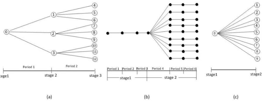
Two important concepts, stage and scenario, should be clarified before we present the model. An information stage, normally simply called stage, is a point in time where decisions are made based on the new information. “It only makes sense to distinguish two points in time as different stages if we observe something relevant (new information) in between” (King and Wallace 2010). The concept of
stage is different from period. Period is the time point where decision can be made regardless the consideration of new information realization. This means we can have more than one period within one stage if no new information is added between the periods. In Fig. 1, (a) is a stage multi-period scenario tree; (b) is a two-stage multi-multi-period scenario tree; while (c) is a two-stage two-multi-period scenario tree. In this work, we study a two-stage multi-period PSP problem as show in (b) in Fig.1. Since there is no new information coming in, i.e. no new random variable realization between each period within each stage, we can aggregate the periods into a stage as shown in Fig.1 (c).
Fig. 1 Examples of scenario trees
The second important concept is scenario. The possible outcomes of the random variables which represent the uncertainty are defined as scenarios. The progressive evolution of the random variables in our two-stage model can be described by a scenario tree as (c) in Fig.1. The root node of the scenario tree represents the initial state at the current time. The discrete evolutions of the random variables during the planning horizon are specified by nodes and arcs. In Fig.1 (c), node n = 1-9 represents each realization of random variables in the second stage, i.e. the state of the market. The arcs represent the possible transitions between two adjacent states. Each path, starting from the root node to leaf nodes, represents one scenario.
[image:4.595.76.524.356.535.2]5
model in this paper, we do not need to enforce this constraint. We define the decision variables on each node, where node 0 belongs to the first stage while nodes 1, 2,.. belong to the second stage.
Scenario generation methods for stochastic programme have been extensively studied in the literature. We apply a simple yet effective method proposed by (Stoyan and Kwon 2010) to generate scenarios for the SMIP model by employing historical market data. The reason is that if market behaviour is representative for a specific historic time interval, then we expect that this pattern will continue in the near future. (Jobst, Mitra et al. 2006) used the same rationale for their portfolio selection model. We investigate the past market asset prices and produce scenarios that fit in an approximation of that function. We refer to (Jobst, Mitra et al. 2006, Stoyan and Kwon 2010) for more information about the scenario generation methods. The information about the historic data that are applied to generate scenarios and number of scenarios generated will be presented in Section 4.
2.2 SMIP model components
The notations applied in this paper are given in Table 1. Table1. Notations
Sets
A The set of assets. Index i,iA
User-specific parameters
The target expected portfolio return after the planning horizon Critical percentile for VaR and CVaR
Deterministic input data
h The initial available capital to invest in the asset market
0 i
w
The initial position (in number of units ) of asset ii
The fixed fee when purchasing asset i
i
The fixed fee when selling asset i
i
The variable cost when purchasing asset i
i
The variable cost when selling asset i
i
The fixed transaction fee
i
The variable transaction cost
k The number of assets held in the portfolio
wmin The minimum hold position
tmin The minimum trading size
F Feasible solution set
Stage (scenario) dependent data
N The set of nodes in the second-stage in Fig.1, index n,nN
pn Probability of node n in the second stage
0 i
P
The price per unit of asset i in the first stagen i
P
The price per unit of asset i at node n in the second stagen
V
The final wealth of the portfolio at node nn
R
The return of the portfolio at node n6
yn Portfolio shortfall in excess of VaR at node n
z The variable in definition of CVaR which equals to VaR in the optimal solution
Decision variables
bi The number of units of asset i purchased in the first stage
si The number of units of asset i sold in the first stage
wi The position (in number of units ) of asset i after transactions in the first stage n
i
b
The number of units of asset i purchased at node n in the second stagen i
s
The number of units of asset i sold at node n in the second stagen i
w
The position (in number of units ) of asset i after transactions in the second stageci Binary variable in the first stage. Is 1 if we hold asset i, 0 otherwise
fi Binary variable in the first stage. Is 1 if we purchase asset i , 0 otherwise
gi Binary variable in the first stage. Is 1 if we sell asset i , 0 otherwise n
i
c
Binary variable in the second stage. Is 1 if we hold asset i at node n , 0 otherwisen i
f
Binary variable in the second stage. Is 1 if we purchase asset i at node n , 0 otherwisen i
g
Binary variable in the second stage. Is 1 if we sell asset i at node n , 0 otherwiseThe basic portfolio selection problem (deterministic) framework can be expressed as:
min risk measure ( ) (1)
s.t reutrn ( )
; (2)
(3)
i
i
i
w
w
w
F
where objective (1) is to minimize the risk of the portfolio. Constraint (2) ensures the expected return.
F in (3) represents the set of feasible portfolios subject to all the related constraints.
2.1.1 Constraint set
In financial practice, the transaction cost has significant effects on portfolio selection. It has been shown in (Arnott and Wagner 1990) that ignoring the transaction cost could result into inefficient portfolios. This has also been justified by experimental studies in (Yoshimoto 1996). If the transaction cost function is linear, which leads to a convex optimisation problem, then the problem is generally easy to solve. However, a function which better reflects realistic transaction costs is usually non-convex (Konno and Wijayanayake 2001). The non-non-convex optimisation problem is more challenging. In this paper, we consider a model that includes a fixed transaction fee plus a linear cost, thus leads to a non-convex function shown in Fig. 2, as the cost decreases relatively when the trading amount increases (Yoshimoto 1996, Konno and Wijayanayake 2001, Konno and Wijayanayake 2002). This function is also applied in (Lobo, Fazel et al. 2007). The transaction cost function is given in (4), and shown in Fig. 2, notations given in Table 1. In this work we aggregate the costs occurred in selling and buying an asset, and use a compact transaction cost function i i ib bi, i 0.
0, 0; , 0; , 0; i
i i i i i
i i i i x
b b s s
7 Fig.2 The transaction cost function (Lobo, Fazel et al. 2007)
Throughout the planning period cash inflows and cash outflows occur due to the assets selling, purchasing and transaction costs associated with asset trading. In other words, this constraint reflects the evolution of the cash balance of the investment over time. The cash balance constraint can be explained by Fig.3.
Fig.3 Cash flow balance
We state the cash balance constraint for the first stage (5) and second stage (6) as the following:
0 0
(1 ) (1 ) (5)
i i i i i i
i A i A
h s P b P
(1 ) (1 ) (6)
n n n n
i i i i i i
i A i A
s P b P n N
We have the asset balance condition for each asset at the first stage (7) and second stage (8): 0
(7)
i i i i
w w b s iA
, (8)
n n n
i i i i
w wb s iA nN
Next, we introduce a binary variable ci and n i
c to control the number of assets to hold at the first stage
and second stage. ci =1 if the investor holds asset i, ci= 0 otherwise. The cardinality constraint states that the portfolio consists of k assets as the following:
(9)
i i A
c k
(10)
n i i A
c k n N
The minimum position constraint prevents investors from holding very small positions after the rebalancing. We introduce a prescribed positive percentage value wmin. That is, holding a position
8
positions can be forbidden by introducing the following constraints for the first stage (11) and second stage (12):
min i i (11)
w c w iA
min , (12)
n n
i i
w c w iA nN
In addition, we introduce a minimum trading constraint to prevent trading a very small amount of assets less than a prescribed percentage value tmin. Two additional sets of binary variables, fi and gi
(and n i
f and n i
g ), are introduced to denote that the investor buys or sells asset i at the first (and second) stage. Similar to the modelling of the minimum position constraint above, the minimum trading constraint can then be expressed as follows:
min min (13) (14) i i i i
t f w i A
t g w i A
min
min
, (15)
, (16)
n n
i i
n n
i i
t f w i A n N
t g w i A n N
We also introduce the exclusive constraint to prevent buying and selling the same asset at the same time:
1 (17) 1 , (18)
i i n n
i i
f g i A
f g i A n N
We denote the final wealth of the portfolio at node n in the scenario tree as n
V , calculated by:
(19)
n n n
i i i A
V P w n N
Based on the final wealth we can define the return of the portfolio as n
R :
0 1 (20)
n n V
R n N
V
Thus we have the expected return constraint as follows:
(21)
n n n N
p R
The integer decision variables , , , n, n, n
i i i i i i
w b s w b s allow identifying the exact number of asset units to purchase or sell at a specific time. However, it dramatically increases computational difficulty. We adapt the same method used in the literature (Gaivoronski, Krylov et al. 2005, Woodside-Oriakhi, Lucas et al. 2013), and set , , , n, n, n
i i i i i i
w b s w b s as real decision variables to represent the fraction invested in asset i in the portfolio. However, the binary integer decision variables c f g ci, , ,i i in,fin,gin
still present great computational difficulty, for which we apply the tailored hybrid algorithm.
2.1.2 Objective function
The conventional MV model applies covariance of the assets in the portfolio as a risk measure, assuming normal distributions in asset returns. However, in practice returns of many financial securities exhibit skewed and leptokurtic distributions (Kaut, Wallace et al. 2007). Many other investments are exposed to multiple risk factors, thus joint effect on portfolio returns often cannot be modelled by a normal distribution. Alternative risk measures have been sought. Such measures, such as Value-at-risk (VaR) (Jorion 2001), are concerned with additional characteristics of the return distribution (e.g., the tails) besides the variance.
9
by Artzner et al. (Artzner, Delbaen et al. 1999). The VaR of a diversified portfolio can be larger than the sum of the VaRs of its constituent asset components (Kaut, Wallace et al. 2007), thus fails to reward diversification. Moreover, when the returns of assets are expressed in terms of discrete distributions (i.e., scenarios), VaR is a non-smooth and non-convex function of the portfolio positions and exhibits multiple local extreme (Rockafellar and Uryasev 2002). Incorporating such functions in mathematical programs is very difficult, thus making the use of VaR impractical in portfolio optimization models (Kaut, Wallace et al. 2007).
To overcome the deficiencies of VaR, suitable alternative risk measures have been sought. (Artzner, Delbaen et al. 1999) discussed the properties that sound risk measures should satisfy, and specified a family of closely related coherent risk measures termed as expected shortfall, mean excess loss, tail VaR, and conditional VaR to quantify the mass in the tail of the distribution beyond VaR. (Rockafellar and Uryasev 2002) introduced a definition of the conditional value-at-risk (CVaR) measure for general distributions, including discrete distributions that exhibit discontinuities, and showed that CVaR is a continuous and convex function of the portfolio positions. Most importantly, they showed that a CVaR optimization model can be formulated as a linear program in the case of discrete distributions of the stochastic input parameters. In this work we choose CVaR as the risk measure.
The objective of our SMIP model is to minimize the expected value of the CVaR in the tail (beyond a specific percentile, ) of the portfolio losses at the end of the planning horizon. CVaR can be transformed to a linear programming (Rockafellar and Uryasev 2000) as the following.
A minimization problem denoted as:
min . .
CVaR s t wF
where w denotes decision variables and F denotes their feasible region, can be reduced to the following linear programming problem:
1 min
(1 )
. . ( , ) ;
0;
n n N
n n
n
z y
n s t y f y z
y
wwhere is a user specified percentile value (e.g. 95%), a parameter for VaR and CVaR. ( ,f x yn) represents portfolio loss over the planning horizon. zis the variable in the definition of CVaR which equals to the optimal VaR value. ynare auxiliary variables in the linear programming formulation which represent the portfolio shortfall (i.e. ( ,f x yn)) in excess of VarR value (i.e. z) at node n.
2.3 SMIP model
10 0
0 0
1
min (SMIP) (1 )
. .
,
,
(1 ) (1 )
(1 ) (1 )
n n n N
i i i i
n n n
i i i i
i i i i i i
i A i A
n n n n
i i i i i i
i A i A
i i A
n i i A
z p y
s t
w w b s i A
w w b s i A n N
h s P b P
s P b P n N
c k c
min min min min min min , , , 11 ,
i i n n i i i i i i n n i i n n i i i i n n i i
n n n
i i i A
k n N
w c w i A
w c w i A n N t f w i A
t g w i A
t f w i A n N
t g w i A n N
f g i A
f g i A n N
V P w n
0 1 0 , , , , , , , , , , , n n n n n n n n Nn n n i i i i i i
n n n
i i i i i i
n
N
V
R n N
V
y R z n N
y n N
p R
w b s w b s R
c f g c f g B z y R
3. Simplification and Hybrid Solution Approach
11
information with regard to cardinality constrained PSP we refer to (Woodside-Oriakhi, Lucas et al. 2011).
Due to the integer variables and the nature of the stochastic model, finding solutions to the two-stage model is challenging. Therefore, a simplification method is applied to accommodate the complexity of our problem models.
A large variety of decomposition methods have been applied to SMIP models. A common strategy in stochastic programing is to decompose the problem based on time-stage or scenarios (Barro and Canestrelli 2005, Escudero, Garín et al. 2007, Shaw, Liu et al. 2008). Stoyan and Kwon (Stoyan and Kwon 2011) decomposed the problem geographically into security and bond problems. The sub-problems are further broken down by relaxing difficult constraints. In our previous work () …
Motivated by this, in this paper, we adapt a simplification method in our previous work for solving … to eliminate the difficult constraints in the SMIP model, leading to easier sub-problems to tackle. Several researchers have pointed out that the cardinality constraint presents the greatest computational challenge to the problem (Bienstock 1996, Jobst, Horniman et al. 2001, Stoyan and Kwon 2010, Stoyan and Kwon 2011). Actually, the PSP with cardinality constraint has been recognized to be NP-complete (Bienstock 1996, Mansini and Speranza 1999).
To eliminate the cardinality constraint, we identify variables ci which define the cardinality constraint
i i A
c k
as a set of core variables. Variable fixing (Bixby, Fenelon et al. 2000) then is applied on this set of core variables ci. There are two benefits after variable fixing. Firstly, the cardinality constraint which is defined by these core variables is eliminated (i.e., each core variable has a value assignment). This reduces the computational complexity. Secondly, sub-problems are generated by variable fixing. Based on the variable fixing, we perform local search on these core variables, which is computationally inexpensive, and then the default Branch-and-Bound search is performed on the sub-problems to generate complete solutions to the original sub-problems. That is, local search and Branch-and-Bound methods are integrated to solve our SMIP models. In this work, we apply variable fixing only on the first-stage variable ci to simplify the problem. How to apply variable fixing on morevariables, i.e. those in the second-stage will be investigated in our future work.
3.1 Framework of Hybrid Local Search and B&B Algorithm
12 Fig. 3
Framework
of LS-B&BLS-B&B consists of four main components. The first component is the initialization phase (line 1). In this phase, variable fixing is applied to generate two branches of sub-problems. Lower bound and upper bound of the problem are also initialized in this phase.
The second component is a default B&B search (line 7). It is called to solve the sub-problems to optimality. From this, the solutions and the objective value of the original problem can be obtained. The third component is a local search (line 9) which is performed on set C of variable ci to update sets
S and S’. With the updated S and S’, the sub-problems are updated correspondingly. Therefore, we state that this local search generates a sequence of sub-problems.
The fourth component is an overall search procedure (while loop), which we name as Local Search B&B. In this search, a local search (i.e., the third component) is applied to generate a sequence of sub-problems. This Local Search B&B search includes the pruning of inferior sub-problems and solving the promising sub-problems to optimality.
We present explanations of key components next.
3.2 Variable fixing
(Hard) variable fixing has been used in MIP to divide a problem into sub-problems (Bixby, Fenelon et al. 2000). It assigns values to a subset of variables of the original problem (Bixby, Fenelon et al. 2000, Lazic, Hanafi et al. 2009). That is, certain variables are fixed to given values. For a given original MIP problem denoted as follows:
: min . . ;
{0,1}, [0,1],
T org
j
j
P c x
s t Ax b
x j B
x j C
where x is the vector of variables. x are partitioned into two subsets: B corresponds to the set of binary variables and C corresponds to the set of continuous variables.
LS- B&B
/* LB: lower bound; UB: upper bound;
(h, x,): a solution (x) of the problem with a corresponding objective value h; solveB&B: a default B&B solver;
C: set of ci;
S and S’: two complementary subsets of C, i.e., S = C/ S’ Porg: original problem defined by model (PSP);
y sub
P ,Psub'y
: sub-problems defined by variable fixing; */ 1: Initialization phase
2:while (the number of iterations not met) // overall search 3: If (LB (
y sub
P ) ≥ UB) 4: prune the sub-problem
y sub
P ; 5: go to line 9;
6: Else
7: (h, x) = solveB&B(
y sub
P ); 8: if h <UB, set UB =h;
9: perform a Local search on the set C; 10: generate sub-problems by variable fixing:
y
sub
P = Porg (ci= 1), ciS; 'y
sub
P = Porg (ci = 0), ciS’;
13
Variable fixing, as its name suggests, fix a restricted subset S of the binary variable to certain values, e.g. 1. Then we have a reduced problem Pr as follows:
: min . . ; 1, {0,1}, \ [0,1], T r j j j
P c x
s t Ax b
x j S B
x j B S
x j C
We denote this problem as a reduced problem because certain binary variables (i.e., the variables in set S) are already fixed. Note that the variables outside the restricted subset S, i.e., variables in B/S, are still free binary variables.
We apply variable fixing to simplify the original problem into sub-problems by fixing variables in the two complementary subsets S and S’, S’=B/S, to 1 and 0, respectively, to obtain two sub-problems
y sub
P and '
y sub
P as the following:
: min . . ; 1, {0,1}, ' [0,1], y T sub j j j
P c x
s t Ax b
x j S B
x j S B
x j C
' : min . . ; 0, ' {0,1}, [0,1], y T sub j j j
P c x
s t Ax b
x j S B
x j S B
x j C
3.3. Initialization phase
The main task of the initialization phase, shown in Fig.4, is the generation of two sub-problems y sub
P
and '
y sub
P by variable fixing on variables ci on sets S and S’. From the definition of
y sub
P , we can state that
y sub
P is the Porg with the initialization of variables in S to 1. And '
y sub
P is the Porg with the
initialization of variables in S’ to 0.
Fig.4.Initialization phase of Local Search B&B approach
In the lines 1 and 2 of the initialization phase, a heuristic is applied to generate a good first sub-problem. This heuristic is based on the first-stage problem of SMIP model where the second-stage
Initialization phase
R: continuous relaxation of the first-stage problem; solve: a quadratic program solver;
C: set of binary variables ci;
S, S’: two complement sets of C, S’ = C/S;
k: the number of assets allowed in the portfolio, as defined in the model (SMIP);
Porg: the original problem defined on model SMIP;
1: solve the continuous relaxation problem R(Porg): solve (R(Porg));
2: sort the assets according to a sort rule;
3: consider the sorted assets to generate sub-problems by variable fixing: 4: select the first k assets and add them into set S;
5: generate two branches of sub-problems by variable fixing: 6:
y sub
P = Porg (ci = 1), ciS;
7:
= Porg (ci = 0), ciS’;8: obtain lower bound of sub-problem
y sub
P , discard 'y sub
P : LB (
y sub
P )= solve(
y sub
14
recourse variables and constraints are dropped off. The integer decision variables ci are relaxed as
continuous ones.
In (Mansini and Speranza 2005), it has been shown that, the set of assets selected by the continuous relaxation problem often contains the assets which are included in the integer optimal solution. Based on this, we apply a heuristic to select the first subset S to construct the first sub-problem
y sub
P as the
following:
1. Relaxed problem solution: solve the continuous relaxed first-stage problem. Save the solution vector w;
2. Sort on the assets: sort the assets in a non-decreasing order of the reduced cost of w of the continuous relaxation to model (Mansini and Speranza 2005);
3. Select the assets: select the first k assets of the solution vector w. These assets form the first sub-problem.
This heuristic is applied in line 2 in the algorithm presented in Fig. 4 to ensure a proper selection of the first sub-problem.
3.4 Local search to generate a sequence of sub-problems
A local search is performed on the set C of variables ci to generate new value assignment for each
variable ci(see pseudo code in Fig. 5). Each move of the local search updates the subsets S and S’ thus
a sequence of sub-problems is created.
Theoretically, any local search technique can be applied to search on ci. In this paper, we apply a
variation of Variable Neighbourhood Search (VNS) (Hansen, Mladenovic et al. 2001) to carry out the search on ci. The evaluation value of solution c and its neighbour are calculated by the continuous
relaxation solution of the problems.
Fig.5 Steps of VNS local search
Three neighbourhood structures Nl are employed in the algorithm. N1 swaps one pair of elements in S
and S’. N2 and N3 swap two and three pairs of elements, respectively. For each current neighbourhood
structure Nl, a given number of it2 iterations are carried out before the search moves to the next
neighbourhood structure Nl+1. This procedure terminates after it1 iterations. Therefore, Local Search
B&B is an incomplete search. It aims to seek near optimal solutions in a limited computational time.
Local search on Z
c: current assignment of ci
e: evaluation value of a solution: e = solve(R( ));
1: Select the set of neighbourhood structures Nl, l = 1, …, lmax;
2: Provide an initial solution vector c (c represents the assignment of zi)
3: Repeat the following steps for it1 iterations:
4: set l =1;
5: Repeat the following steps for it2 iterations:
6: Exploration of the neighbourhood Nl of z with the aim to update the assignment of ci: Find the first improved
neighbour c’ of c;
15
3.5 The overall search procedure on the sequence of sub-problems
The overall search explores on this sequence of sub-problems. This is shown in the while loop in Fig.3. In this search, the lower bound of the sub-problem
y sub
P is computed by a general LP solver,
which relaxes the sub-problem to a continuous problem (line 3 in Fig.3). The objective value of the feasible solution to the concerned sub-problem
y sub
P serves as the upper bound of the original problem. If the lower bound of a sub-problem is above the current upper bound found so far, we can prune this sub-problem during the search (line 4 in Fig.3). Otherwise, these sub-problems are solved exactly by a default B&B in an IP solver (line 7 in Fig.3). The solutions to the sub-problems together with the assignments of core variables consist of the feasible solutions to the complete original problem. These sub-problems are solved in sequence and the best solution among them approximates the optimal solution to the original problem. The whole procedure terminates by terminating the generation of sub-problems by the local search. Therefore, the search is an incomplete search. It cannot guarantee optimality of the solution due to the nature of the local search on core variables ci.
4. Experimental results
We implement our two-stage stochastic mixed integer program model in C++ with concert technology in CPLEX on top of CPLEX12.3 solver on a set of benchmark instances. The aims of our experiments are: firstly, to investigate the efficiency of the proposed hybrid method for generating good solutions in a reasonable computational time; and secondly, to evaluate the performance of the two-stage stochastic model.
4.1 Test problems
In this paper, we investigate the multi-period PSP with a comprehensive set of real-world trading constraints, together with market uncertainty. We evaluate our algorithm on five general benchmark
instances (see Table 2) which are publicly available in the OR library at
[image:15.595.244.352.564.639.2]http://people.brunel.ac.uk/~mastjjb/jeb/info.html, We extend the problems with additional constraints derived from a real-world problem at Société Générale Corporate & Investment Bank. We use the 261 weekly historical price data for each asset to obtain scenarios for the SMIP model. We generate market asset price scenarios for the SMIP model using the framework presented in (Stoyan and Kwon 2010) based on the 261 weekly historical price data for each asset. A similar approximation technique is used in (Jobst, Mitra et al. 2006).
Table.2 Properties of problem instances. m : the total number of assets available; k : the number of assets to be held.
Instance m k Hang Seng 31 10
DAX 85 40
FTSE 89 50 S&P 98 60 Nikkei 225 150
We set the minimum proportion of wealth to be invested in an asset, wmin, to 0.01% and the minimum
transaction amount, xmin, to 0.01%. We also set the parameters in the transaction cost function ßi to
16
4.2 Evaluations on hybrid LS-B&B algorithm
In this section, we analyse our proposed hybrid local search and B&B algorithm for SMIP from different aspects, including sub-problem solving and overall problem solving. The hybrid local search and B&B algorithm is implemented in C++ with concert technology in CPLEX on top of CPLEX12.3 solver. All experiments have been carried out on an Intel Core Duo machine with CPU @ 3.16GHz 3.17GHz and 2.97GB memory.
4.2.1 The size of the original problem and sub-problems
First, we evaluate the effectiveness of the problem simplification of the variable fixing on the SMIP model. The original problem is SMIP and sub-problems are still MIP due to the binary variablesf gi, i. We compare the size of the original problem and sub-problems after the variable fixing in Table 3. Due to the variables needed to define each scenario at each node, the size of the original problem is very large. After fixing the values for all variables ci by variable fixing, the resulting sub-problems
are much smaller than the original ones. We can also observe that the size of the sub-problems are similar (Table 3 presents the approximate average size of sub-problems). Note that in this work we aim to reduce the computational time of solving the problem by heuristically simplifying the original problem. As the problem size is reduced by using variable fixing on ci, the sub-problems can be
[image:16.595.136.460.367.466.2]solved efficiently by the default B&B in CPLEX 12.3 in our experiments.
Table 2. Size of the original SMIP problem and the approximate average size of SMIP sub-problems
Instance Original problem Sub-problem No. of
rows
No. of columns
No. of nonzeros
No. of rows
No. of columns
No. of nonzeros Hang Seng 22790 22560 78722 11364 11210 39789 DAX 74109 73734 264652 38451 38412 154784 FTSE 78989 78606 282408 41254 40245 120354 S&P 90649 90191 324538 43214 42145 117453 Nikkei 321181 320470 1171936 154876 157489 547890
4.2.2 Computational anlysis of the sub-problem solving
In this section, we analyse the deferent performance (i.e., CPU time spend) of the sub-problem solving. In the LS-B&B algorithm in Fig.3, after the simplification, the sub-problems are solved by default B&B. With the calculation of the lower bound and upper bound in the search, some sub-problem can be pruned. Actually, when these sub-sub-problems are processed, four possible situations could emerge: (1) a sub-problem could be solved by B&B to optimality; (2) the repairing heuristic imbedded in CPLEX could be evoked and applied to a sub-problem to obtain a feasible solution heuristically; (3) a sub-problem could be pruned; this will happen if the optimal solution under LP relaxation is larger than the current upper bound; and (4) the solution of a sub-problem could be infeasible.
Table 4. Computational analysis on sub-problem processing.
Instance
Avg CPU time per sub-p for sub-problem
solved
Avg CPU time per sub-p for sub-problem
repaired
Avg CPU time per sub-p for sub-problem
pruned
Avg CPU time per sub-p for sub-problem
infeasible Hang
Seng
0.76 0.07 0.1 0
DAX 1.2 0.1 0.1 0
FTSE 0.88 0.75 0.2 0
S&P 1.40 0.6 0.2 0
[image:16.595.74.528.660.769.2]17
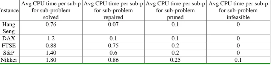
Table 4 clearly indicates that the CPU time for identifying infeasibility is negligible. The more sun-problems pruned, the more efficient the search is. The CPU time for pruning the inferior sub-problem (by calculating its optimal solution of the LP relaxation) is quite efficient.
4.3 Evaluations on SMIP model solutions
In Section 4.2, we analyse the proposed LS-B&B from the aspects of solving the sub-problems and the overall problem. In this section, we examine the performance of the SMIP model and solutions generated by the proposed LS-B&B in static as well as in dynamic tests.
4.3.1 Static tests on SMIP model solutions
It is worth noting that LS-B&B is a heuristic approach. It cannot prove optimality of the solution to the overall problem due to the nature of the local search on core variables zi, although the
sub-problems can be measured by an optimality gap. In order to evaluate the quality of the solutions we obtained from LS-B&B, we compare it against the approximate optimal solution to the problem. It is very difficult, if not impossible, to obtain and prove the optimal solutions to the problems concerned. We therefore calculate the approximate optimal solution to the problem concerned by running the default B&B algorithm in CPLEX12.3 for an extensive amount of time.
We run our hybrid algorithm and default B&B in CPLEX on the same instances with the parameters setting stated above (wmin, xmin,µ etc.), for a given same expected return µ. We calculate the CVaR at
level =95% of portfolio loss.
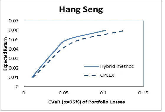
We present the results of hybrid LS-B&B in comparison with the default B&B in CPLEX 12.3 and consider the solution quality and CPU time over the test instances. The two methods solve the same model, that is, employing the same risk measure (CVaR of the portfolio loss), starting with the same initial portfolio. We plot the resulting risk-return efficient frontiers of the two methods in Fig. 6 for the Hang Send instance. From Fig. 6, we can see that the solution obtained by the hybrid method dominates the solution of the default CPLEX method. For any expected return target, the hybrid method can obtain better solution where risk is lower than the solution from CPLEX.
Fig. 6 Efficient frontiers from the hybrid LS-B&B and pure B&B in CPLEX
[image:17.595.160.440.493.683.2]18
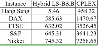
[image:18.595.220.377.176.250.2]solutions in Fig. 6 is presented in Table 5. For larger instances it is very time consuming to plot even a single point on the frontiers. For example, CPLEX needs 7258 seconds to plot one portfolio. The hybrid LS-B&B significantly outperforms the default CPLEX in all of the instances. In the worst case, CPLEX obtains a feasible solution in 7258.65 seconds while the hybrid method only needs 745.32 seconds.
Table 5. Comparison on CPU time between the hybrid LS-B&B method and CPLEX (in seconds).
Instance Hybrid LS-B&B CPLEX Hang Seng 5.46 458.32
DAX 585.63 1470.67 FTSE 632.02 3526.45 S&P 645.31 3641.23 Nikkei 745.32 7258.65
4.3.2 Dynamic tests on portfolio return values
The static test results in Fig. 6 present information on the solution quality at certain points of time in the planning horizon. However, in practice, investors seldom make decisions and evaluate the constructed portfolios based on a single static result. We run dynamic tests to evaluate the constructed portfolios. This dynamic test reflects information on the solution quality in a more practical manner. In (Topaloglou, Vladimirou et al. 2008), authors ran dynamic tests to assess the performance of the models in backtracking simulations. The key idea of the test method is to compare the results (i.e. return values) that have been generated by the model with the actual return values. This is a widely-used method, with several variants, to evaluate algorithm performance in the Stochastic Programming literature (Fleten, Høyland et al. 2002, Stoyan and Kwon 2010, Stoyan and Kwon 2011). In this section, we adapt the same idea to evaluate solutions generated by the proposed LS-B&B for the two-stage SMIP model.
One of the methods an investor evaluates the performance of a portfolio is comparing the portfolio values against a well-known benchmark index. This is called index tracking, a well-known passive investment strategy (Canakgoz and Beasley 2009). In this section, we illustrate the performance and strengths of the proposed stochastic model by presenting the obtained portfolio values against the
actual market index value.
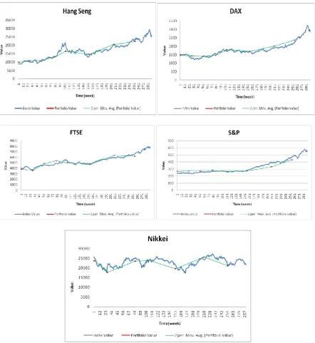
In Fig 7, for each index of the five world-wide index markets, we have 291 weekly (5 years) index values (solid lines). Our SMIP model was run, on a rolling horizon basis, at intervals of every six months. Starting from week one, the model is run to decide the assets and their positions in the portfolio, as well as the value of the portfolio. Then time moves forward 6 months and the model is run again to obtain new portfolios. Therefore, we can plot 10 points of the constructed portfolio values (with six-month intervals over 5 years), obtained by the SMIP model.
19 Fig. 7 Portfolio values from the SMIP model against the market index values
[image:19.595.76.519.69.551.2]In order to observe closer details in Fig. 7, we present the detailed data in Table. 6. The left column presents the absolution difference between the index value Vindex and portfolio value Vportfolio. The right column presents the percentage difference between the index value and portfolio value, from which we can see that for three instances (Hang Seng, DAX and S&P), our method obtained slightly better solutions on average. For instance FTSE, the portfolio values are worse than the index values, however at a negligible difference.
Table 6.Comparisons between portfolio value from the SMIP model and index value
Instance Absolute Value(=VportfolioVindex) Percentage Value(=(VportfolioVindex) /Vindex)
Best Worst Average S.D Best Worst Average S.D. Hang Seng 1679.3 -3858.2 -96.3753 1479.203 0.137656 -0.18894 0.015966 0.094567
[image:19.595.70.532.711.768.2]20 FTSE 444.52 -547.02 -40.8275 340.819 0.091175 -0.08152 -0.00853 0.065765 S&P 31.978 -67.767 -3.61219 33.12401 0.132128 -0.16952 0.008566 0.099073 Nikkei 1362.3 -3779.9 -940.907 1551.7 0.056132 -0.17479 -0.04167 0.068627
The evaluation method applied above, i.e. comparing the return values obtained from the model against actual market values, is a reasonable and well-justified method for the following reasons: (1) Comparing the results obtained from the model with the actual market values is convincing since facts speak for themselves. (2) The portfolio selection problem is one of the most studied topics in finance. A wide range of models have been proposed to tackle the problems. Different variable definitions, objective functions, constraints, and data sets have been proposed. It is therefore difficult to conduct fair and exhaustive comparisons of all the published work. What is more, to the best of our knowledge, our two-stage SMIP model with the comprehensive set of constraints, as well as uncertainties by employing scenarios, is presented in the literature for the first time. There is no existing work we could conduct comparisons against our hybrid LS-B&B approach on the same data. (3) The nature of SP models, i.e. the randomness, make it difficult or even impossible to make parallel comparing, i.e., comparing with other methods in the literature.
5. Conclusions
In this paper, we investigate a multi-period portfolio selection problem under random uncertainty in term of asset price and with a comprehensive set of real-world constraints. We formulate the problem into a two-stage stochastic mixed-integer program, and apply a hybrid method, where a simplification method and a local search with B&B are employed. The hybrid local search and B&B method can obtain good solutions for the highly computational expensive problem in less computational time comparing with default B&B.
The stochastic mixed-integer programming model manages the risk by minimizing the conditional value at risk (CVaR) of portfolio loss. We run static and dynamic experiments to investigate the performance of the model. We demonstrate that the constructed portfolio value can match the market index with holding of less number of assets.
The stochastic model provides a flexible framework to multi-period portfolio optimization. In this work, we test and analyse the performance of the two-stage model. In our future work, we will analyse qualitatively in what ways the optimal solution changes as the uncertainty is introduced. We will also investigate alternative objective functions to reflect investors’ preferences and incorporate additional practical constraints.
References
Arnott, R. D. and W. H. Wagner (1990). The measurement and control of trading costs. Financial analusts journal4(6): 73-80.
Artzner, P., F. Delbaen, J. M. Eber and D. Heath (1999). Coherent measures of risk. Mathematical Finance9(3): 203-228.
Baldacci, R., M. A. Boschetti, N. Christofides and S. Christofides (2009). Exact methods for large-scale multi-period financial planning problems. Computational Management Science6(3): 281-306. Barro, D. and E. Canestrelli (2005). Dynamic portfolio optimization: Time decomposition using the Maximum Principle with a scenario approach. European Journal of Operational Research 163(1): 217-229.
Bienstock, D. (1996). Computational study of a family of mixed-integer quadratic programming problems. Mathematical Programming74(2): 121-140.
21 Bixby, R., M. Fenelon, Z. Gu, E. Rothberg and R. Wunderling (2000). MIP:Theory and practice--closing the gap. System Modelling and Optimization: Methods,Theory and Applications174: 19-49.
Canakgoz, N. A. and J. E. Beasley (2009). Mixed-integer programming approaches for index tracking and enhanced indexation. European Journal of Operational Research196(1): 384-399.
Chang, T. J., N. Meade, J. E. Beasley and Y. M. Sharaiha (2000). Heuristics for cardinality constrained portfolio optimisation. Computers & Operations Research27(13): 1271-1302.
Crama, Y. and M. Schyns (2003). Simulated annealing for complex portfolio selection problems.
European Journal of Operational Research150(3): 546-571.
Escudero, L. F., A. Garín, M. Merino and G. Pérez (2007). A two-stage stochastic integer programming approach as a mixture of Branch-and-Fix Coordination and Benders Decomposition schemes. Annals of Operations Research152(1): 395-420.
Fleten, S.-E., K. Høyland and S. W. Wallace (2002). The performance of stochastic dynamic and fixed mix portfolio models. European Journal of Operational Research140(1): 37-49.
Gaivoronski, A. A., S. Krylov and N. van der Wijst (2005). Optimal portfolio selection and dynamic benchmark tracking. European Journal of Operational Research163(1): 115-131.
Gupta, P., M. Inuiguchi, M. K. Mehlawat and G. Mittal (2013). Multiobjective credibilistic portfolio selection model with fuzzy chance-constraints. Information Sciences229(0): 1-17.
Gupta, P., M. K. Mehlawat and A. Saxena (2010). A hybrid approach to asset allocation with simultaneous consideration of suitability and optimality. Information Sciences180(11): 2264-2285. Hansen, P., N. Mladenovic and D. Urosevic (2001). Variable neighborhood search: Principles and applications. European Journal of Operational Research130(3): 449-467.
He, F., R. Qu and E.Tsang (2013). Hybridising Local Search with Branch-and-Bound for Constrained Portfolio Selection Problems. Technique report, School of Computer Science, University of Nottingham.
Higle, J. L. and S. W. Wallace (2003). Sensitivity Analysis and Uncertainty in Linear Programming.
Interfaces33(4): 53-60.
Ji, X., S. Zhu, S. Wang and S. Zhang (2005). A stochastic linear goal programming approach to multistage portfolio management based on scenario generation via linear programming. IIE Transactions37(10): 957-969.
Jobst, N. J., M. D. Horniman, C. A. Lucas and G. Mitra (2001). Computational aspects of alternative portfolio selection models in the presence of discrete asset choice constraints Quantitative Finance 1(5): 489-501.
Jobst, N. J., G. Mitra and S. A. Zenios (2006). Integrating market and credit risk: A simulation and optimisation perspective. Journal of Banking & Finance30(2): 717-742.
Jorion, P. (2001). Value at Risk: The New Benchmark for Managing Financial Risk. New York, McGraw-Hill.
Kaut, M., S. W. Wallace, H. Vladimirou and S. Zenios (2007). Stability analysis of portfolio management with conditional value-at-risk. Quantitative Finance7(4): 397-409.
Kellerer, H., R. Mansini and M. G. Speranza (2000). Selecting Portfolios with Fixed Costs and Minimum Transaction Lots. Annals of Operations Research99(1): 287-304.
King, A. J. and S. W. Wallace (2010). Modeling with Stochastic Programming.
King, A. J. and S. W. Wallace (2012). Modeling with Stochastics Programming, Springer.
Konno, H. and A. Wijayanayake (2001). Portfolio optimization problem under concave transaction costs and minimal transaction unit constraints. Mathematical Programming89(2): 233-250.
Konno, H. and A. Wijayanayake (2002). Portfolio optimization under D.C. transaction costs and minimal transaction unit constraints. Journal of Global Optimization22(1): 137-154.
22 Li, J. and J. Xu (2013). Multi-objective portfolio selection model with fuzzy random returns and a compromise approach-based genetic algorithm. Information Sciences220(0): 507-521.
Lobo, M., M. Fazel and S. Boyd (2007). Portfolio Optimization with Linear and Fixed Transaction Costs. Annals of Operations Research152(1): 341-365.
Mansini, R. and M. G. Speranza (1999). Heuristic algorithms for the portfolio selection problem with minimum transaction lots. European Journal of Operational Research114(2): 219-233.
Mansini, R. and M. G. Speranza (2005). An exact approach for portfolio selection with transaction costs and rounds. IIE Transactions37: 919-929.
Markowitz, H. M. (1952). Portfolio Selection. J. Finance7: 77-91.
Mulvey, J. M. and A. Ruszczyński (1995). A New Scenario Decomposition Method for Large-Scale Stochastic Optimization. Operations Research43(3): 477-490.
Mulvey, J. M. and H. Vladimirou (1992). Stochastic Network Programming for Financial Planning Problems. Management Science38(11): 1642-1664.
Rockafellar, R. T. and S. Uryasev (2000). Optimization of Conditional Value-at-Risk. The Journal of Risk2(3): 21-41.
Rockafellar, R. T. and S. Uryasev (2002). Conditional value-at-risk for general distributions. Journal of Banking and Finance26(7): 1443-1471.
Shaw, D. X., S. Liu and L. Kopman (2008). Lagrangian relaxation procedure for cardinality-constrained portfolio optimization. Optimization Methods & Software23: 411-420.
Stoyan, S. and R. Kwon (2010). A two-stage stochastic mixed-integer programming approach to the index tracking problem. Optimization and Engineering11(2): 247-275.
Stoyan, S. J. and R. H. Kwon (2011). A Stochastic-Goal Mixed-Integer Programming approach for integrated stock and bond portfolio optimization. Comput. Ind. Eng.61(4): 1285-1295.
Topaloglou, N., H. Vladimirou and S. A. Zenios (2008). A dynamic stochastic programming model for international portfolio management. European Journal of Operational Research185(3): 1501-1524. Vielma, J. P., S. Ahmed and G. L. Nemhauser (2008). A lifted linear programming branchand-bound algorithm for mixed-integer conic quadratic programs. INFORMS Journal on Computing20: 438-450. Woodside-Oriakhi, M., C. Lucas and J. E. Beasley (2011). Heuristic algorithms for the cardinality constrained efficient frontier. European Journal of Operational Research213(3): 538-550.
Woodside-Oriakhi, M., C. Lucas and J. E. Beasley (2013). Portfolio rebalancing with an investment horizon and transaction costs. Omega41(2): 406-420.