doi:10.4236/ijcns.2009.25039 Published Online August 2009 (http://www.SciRP.org/journal/ijcns/).
Research on Error’s Distribution in Triangle
Location Algorithm
Jian ZHU, Hai ZHAO, Jiuqiang XU, Yuanyuan ZHANG
The Northeast University, Shenyang, China Email: zhujian1981710@163.com
Received July 18, 2008; revised February 18, 2009; accepted March 27, 2009
ABSTRACT
The error will inevitably appear in triangle location in WSNs (wireless sensor networks), and the analysis of its character is very important for a reliable location algorithm. To research the error in triangle location al-gorithm, firstly, a triangle location model is set up; secondly, the condition of the minimal error is got based on the analysis of the location model; at last, by analyzing the condition, the law of error’s changing is ab-stracted, and its correctness is validated by some testing. The conclusions in this paper are all proved, and they provide a powerful foundation and support for reliable location algorithm’s research.
Keywords: Localization, Error Distribution, Triangle, MicaZ, WSNs
1. Introduction
The information usually binds with the node’s position in pervasive computing [1,2] as approximately 80% infor-mation is related with position in this computation [3]. Therefore, the location study becomes an essential topic in pervasive computing [4]. Nowadays, most existing location algorithms [5-7] contain two basic steps: 1) distance (or angle) measurement; 2) location computa-tion.
Currently, the triangle location is a hot research topic [8,9]. Because of the unavoidable location error, the key problem of reliable location is how to decrease the error as much as possible. But many literatures about the tri-angle location are lack of researches on the change law of location error, and they did not consider the error’s distribution in a triangle. This article draws a conclusion: the error’s change in triangle is stochastic, and the errors in different position are different. If a location algorithm has not considered the error’s changing law, its applica-tion scope will be confined or even can not be applied at all. So, the analysis of error is very important for a reli-able triangle location algorithm.
2. Mathematical Model of Location Question
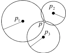
In the three-dimensional space, it can determine the co-ordinate of a location point according to the distance from the location point to four reference points, and this is the same with the basic principle of global positioning system (GPS) [10]. In pervasive computing, however, the most coordinate systems are two-dimensional space and they also do not need the clock synchronization. Therefore, it can fix on the position of a location point as long as the distance from this location point to three ref-erence points is known. As shown in Figure 1, the basic principle of trilateral location is the solution of three cir-cles’ intersection whose radii and the coordinate of circle center are known.
p
2
p
3
p
1
[image:1.595.356.489.596.703.2]p
Due to the limit of pervasive terminal's hardware and energy consumption, the ranging error between nodes is usually biggish. Here, it supposes the ranging error's scope is in (0, ±) and takes (>0). So three circles are no longer intersect at a point, but constitute a small region, denoted by Cp. Supposes the coordinate of the point to be located p is (x, y), then it can locate this point and get three reference points denoted by pi which constitutes the triangle. The coordinate of pi is respectively (xi, yi), i=1, 2, 3, the distance to the location point is ri, and i is the ranging error, makes Cpi, Cp and Sp:
} ) ( ) ( ) ( , ) ( ) ( ) ( | ) , {( 2 2 2 2 2 2 i i i i i i i i p r y y x x r y y x x y x C i (1) } , | ) , {( 3 1 3 1
i p i pp x y x C i y C i
C (2)
} 0 , | ) ,
{( 2 2 2
i i
p x y x y
S i (3)
In order to simplify the analysis, supposes ranging er-ror is equal, namely i=, i=1,2,3, then, when 0, the set of points Cp in Formula (2) will assemble into one point (e.g. Figure 1); However, when >0, Cp will be a convex small region, and its area represents location error size, as shown in Figure 2.
[image:2.595.89.285.214.306.2]1
p
2p
3p
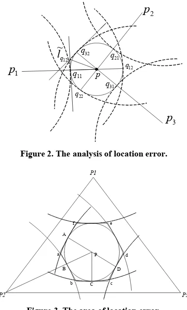
22 q 12 q 31 q 21 q 32 q p 12 ~ q l 11 qFigure 2. The analysis of location error.
[image:2.595.75.268.396.716.2]P2 P3 P1 A B C d e f P c b a D
Figure 3. The area of location error.
In the figure above, supposes lppi is a straight line which pasts point p, pi and intersects the circle Sp in Formula (3) at two points qij, j=1, 2. Make tangent lqij for Sp pasting qij, then the tangent will intersect as arbitrary hexagon like Figure 3, and region Cpi is between the straight line lqi1 and lqi2. Take Cp=Cp 1∩Cp2∩Cp3, then the final Cp will be the hexagon abcdef in Figure 3. The area of Cp edge can be linearized as measuring error is less, and it will be estimated as Cp, namely Cp will ap-proximately be regard as Cp, it may also find in Figure 3 that the Cp region cut by arc is almost the same with hexagon region Cp. Thus, the node location question in the two-dimensional space is transformed into discussing how to arrange three reference points for minimizing the area S (Cp) of region Cp.
3. Condition of Minimum Location Error
Lemma 1: Supposes a, b, c is three numbers whose value is bigger than 0, thenabc3 abc and the equal
sign holds only when a=b=c.
Supposes α1, α2, α3 is respectively the angle (central angle) between vector PA and PB, PB and PC, PC and PD. The region constituted by Cp is a circumscribed hexagon of circle Sp as shown in Figure 3, then
) 2 tan 2 tan 2 (tan 2 ) ~
( 2 1 2 3
p C
S (4)
As to α1, α2, α3, it has the following relationship:
1 2 3
when 0xπ/2, then (tan x)=2tanx(1+tanx)0, and we may derive the following expression using Lemma 1:
3 1 2 3
2 3 2 1 2 2 tan 2 tan 2 tan 6 ) 2 tan 2 tan 2 (tan 3 1 6 ) ~ ( a a a C S p (5)
The equality above holds only when α1 = α2 = α3=π/3, namely conclusion 1: S (Cp) can obtain the minimum value only when α1 = α2 = α3.
As α1 = α2 = α3=π/3, it is not difficult to deduce ac-cording to the geometry principle that the angle of three linked lines formed by three reference points and a point to be located P is mutually 120°. Therefore, only when the angle of three linked lines formed by three reference points and the point to be located is mutually 120°, error zone Cp can become the circumscribe hexagon of the circle. In this case, the location error of the location point can achieve minimum, and this conclusion is the so-called formation condition of the minimum location error.
one error zone of the point to be located presents hexa-gon at most, and the location error increases along with the distance from this point to point P. For instance, as the location point is S and its error zone is an anomalous hexagon; its error zone area will be obviously bigger than the error zone area of point P.
4. The Change Law of Location Error
Take Figure 4 as an example, after the offset of arbitrary point (S) and the minimum error point (P), all three an-gles formed mutually by point S and three reference points of the triangle will change. Supposes α4, α5, α6 is respectively the angle formed by intersection of vector Sa and Sb, Sb and Sc, Sc and Sd. According to computa-tion, the location error zone area of point S is:
P2
P3
P
P1
S a
b
c d A
B
C D
[image:3.595.64.285.290.449.2]e
Figure 4. The location error of random position.
p/6 y
A B
G
D Y=tanx
Y=x
F C F1
G1
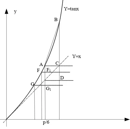
Figure 5. The rule of location error’s increase.
) 2 tan 2 tan 2 (tan 2 ) ~
( 2 4 5 6
S C
S (6)
After the change of point S, α4, α5 and α6 are all changed compared with α1, α2, α3 in the Formula (4), supposed these three angles’ variation is α4, α5,
α6, then there must be increment and decrement among them, and the sum of these three variation should be 0 .meanwhile, the size of 4, 5, 6 is decided by the angle which is formed mutually by point S and three reference points. For instance, angle P1SP2 in Fig-ure 4 is equal to the sum of α4 and α6, it means the sum of α4 and α6 will be smaller as angle P1SP2 gets smaller, and as the sum of α4, α5 and α6 is 180° based on the pre-ceding text, the value of α5 will be bigger.
α α α
The angle of point S and three reference points is not equal to 120°, and α4/2, α5/2 and α6/2 is not equal to 30°.
α5 in Figure 4 is increment, and the other two are dec-rement. The error zone area can reach its minimum value when α1/2, α2/2 and α3/2 are all equal to 30° in terms of the Formula (5). For the quantitative investigation on relationship between the central angle variation of hexa-gon and the error zone area, this article has made the following deduction:x
x 2
cos 1
tan' (7)
The Formula (7) is the derivative formula of tangent function, when x is 0, the tangent derivative value is 1, namely when tangent function in (0, 0) the tangent slope is the same with the slope of y=x. Tangent slope of tan-gent function will be bigger than 1 ifx(0,/2), and it increases along with the increase of x, as shown in Fig-ure 5.
In Figure 5, A is a point whose abscissa is π/6 on the tangent function curve, and the abscissa of point B is equal to a radian corresponds to α5 in Formula (6); the ordinate is tan (π/6+α5). BC is the variation of tangent function corresponds to α5, makes the slope of straight line AB as KAB, then KAB>KFA>KGA. Since BC=α5KAB, AF1=α4KAF and AG1=α6KAG, supposes BC>AF1+ AG1, then after the angle in Formula (4) change into the angle in Formula (6), the variation of the error zone area is:
) (
2 ) ~
(C 2 BC AF1 AG1
S S
(8)
Because:
BC a K a a K
K a K a K a K a AG AF
AB AB
AB AB
AG AF
5 6
4
6 4
6 4
1 1
) (
[image:3.595.64.282.491.708.2]also seen from the figure above, BC is to be bigger if α5 enlarged, meanwhile, it deduces that along with the increase of α5 the error zone area will also increase, the deduce process is as follows:
Supposes α4≤ α 6, then KAG≤KAF, therefore:
AF AF
AG
AG AF
K a K K a
K a K a AG AF
6 6
6 4
1 1
)
(
(9)
In the above expression, AF1+AG1= α6KAF only when α4= α6 and KAG=KAF, and α6= α5/2 holds at this time according to the geometry principle, so the variation of error zone area here can express as:
) 2 / (
2 ) 2 (
2
) (
2 ) ~ (
2 5 5 5
2
1 1 2
AF AB AF
AB S
K K a a K a K
AG AF BC C
S
(10)
In the above expression, as α5 gets bigger, KAB in-creases, KAF reduces, then we may get from the tangent function characteristic that the difference of KAB and KAF/2 will increase along with α5, and the variation of error zone area will increase if α5 enlarged.
Therefore, it can draw the conclusion 2: after an arbi-trary location point offset with the minimum location error point P, once one or two central angles’ degree in-crease which among 6 central angles of the new formed hexagon, the error zone will be bigger along with the increase amplitude of the central angle, and
)
~ ( S
aLim SC .
Synthesizes the above conclusion and Figure 4, it can be seen that when α5 approaches to π, straight line be will be parallel with straight line ce, and the area of quadran-gle Sbec will be close to infinity. Therefore, the final error zone area will be also close to infinitely.
5. Application of the Location Error Change Law
According to the conclusion above, since distribution of the location error in a triangle is stochastic, it will defi-nitely appear the maximum location error and the mini-mum location error in a triangle. The minimini-mum location error in a triangle can only appear on one point, whereas the maximum location error influences positioning sys-tem's accuracy directly, as a result, this article has con-ducted a research to the layout shape of the reference point in view of the maximum location error.
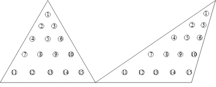
As shown in Figure 6, there are two different kinds of reference point layout schemes under the premise of the same coverage area.
P and P1 is respectively minimum error point in two triangles, as the point to be located S in ABC ap-proaches to point A, angle BSC can only reduce to 60° at most, and according to the relation between central angle and included angle in Figure 4, since point S arrives at
C A 1
P 1 A
P
P1
B
S
[image:4.595.317.534.78.228.2]D
Figure 6. The two way of reference nodes’ layout.
1
2 3
4 5 6
7 8 9 10
11 12 13 14 15
1
2 3
4 5 6
7 8 9 10
11 12 13 14 15
Figure 7. Two way of reference node’s layout.
point A, three central angles will be respectively 30°,30°,120°; as the point D in A1BC approaches to point B, angle A1DC can reduce to the value which is smaller than 60°, it is not difficult by the geometry prin-ciple to deduce that if point D arrives at point B, three central angles will be respectively smaller than 30°, smaller than 30°, bigger than 120°, and the location error of point A in
ABC is bigger than the location error of point B in A1BC by conclusion 2. Point A is the maximum error point in ABC, and the error of point B in A1BC is bigger than the maximum error in ABC, so this article obtains the inference 1: The equi-lateral triangle positioning system's accuracy is higher than non-equilateral triangle positioning system under the same condition.
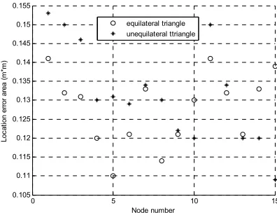
In order to verify the above deduction, this article de-signs an experiment as following figure. Under the plat-form of MicaZ node, laying the point to be located uni-formly in the region encircled by three reference points, the layout graph is as follows:
[image:4.595.314.534.267.356.2]
Table 1. The detailed parameters of nodes in NS-2.
Parameter Value
Nodes distribution As Figure 7
Channel bandwidth 250kbps
Frequency 2.4GHz
Wireless model Shadowing
MAC protocol IEEE 802.15.4
Power for transmission (mwatt) 2.0
Power for idle (mwatt) 1.0
Power for reception(mwatt) 1.0
Power for sleep (mwatt) 0.001
Power for sleep/idle transition (mwatt) 0.2
Time for sleep/idle transition (s) 0.005
0 20
40 60 80
100
0 50
100 0.6 0.65 0.7 0.75 0.8 0.85 0.9 0.95 1
X X: 47.37 Y: 26.32 Z: 0.82
Y
A
O
B
C triangle obviously. Therefore, inference 1 is correct, and
it also indicates the analysis on the error change law in this article conforms to reality.
An experiment is designed to research the distribution of error in a triangle, the platform is the same with the above, and the result is shown in Figure 9:
In Figure 9, the axis X and Y construct a 100m×100m area, ABO is in the area; Axis Z is the precision of location in a triangle. It is shown in Figure 9 that, the precision in the center of a triangle is higher than the fringe areas. So, while in applications, it is better that, keep the unknown nodes in the center area of the three reference nodes.
[image:5.595.146.464.104.377.2]
Figure 9. The precision in the center of a triangle.
6. Conclusions
point in arbitrary triangle according to the theory deduce. The change law of error was verified by practical test, and the research results indicate that the change law of error studied in this article may provide basis and theory instruction for the high performance and reliable location algorithm.
This article mainly studied the formation condition of minimum error and the changing law of error on location
0 5 10 15
0.105 0.11 0.115 0.12 0.125 0.13 0.135 0.14 0.145 0.15 0.155
Node number
Loc
at
ion
err
or
ar
ea (
m
*m
)
equilateral triangle unequilateral ttriangle
7. References
[1] W. K. Edwards, “Discovery systems in ubiquitous co- mputing,” IEEE Pervasive Computing [J], Vol. 5, No. 2, pp. 70-77, 2006.
[2] R. Milner, “Ubiquitous computing: Shall we understand it? [J],” Computer Journal, Vol. 49, No. 4, pp. 383-389, 2006.
[3] J. Y. Junq, “Human-centred event description for ubiquitous service computing [A],” 2007 International
[image:5.595.72.270.551.703.2]Conference on Multimedia and Ubiquitous Engineering [C], pp. 1147-1151, 2007.
[4] D. Noh and H. Shin, “An effective resource discovery in mobile ad-hoc network for ubiquitous computing [J],” Journal of KiSS: Computer Systems and Theory, Vol. 33, No. 9, pp. 666-676, 2006.
[5] G. M. Huang, “A novel TDOA location algorithm for passive radar [C],” CIE international Conference of Radar Proceedings, pp. 41484-41888, 2007.
[6] G. V. Zaruba, “Indoor location tracking using RSSI rea- dings from a single Wi-Fi access point [J],” Wireless Networks, Vol. 13, No. 2, pp. 221-235, 2007.
[7] J. Su, “Location technology research under the environment of WLAN [J],” WSEAS Transactions on Computers, Vol. 6, No. 8, pp. 1050-1055, 2007.
[8] J. Ding, L. R. Hitt, and X. M. Zhang, “Markov chains and dynamic geometry of polygons [J],” Linear Algebra and Its Applications, pp. 255-270, 2003.
[9] J. Ding, L. R. Hitt, and X. M. Zhang , “Sierpinski pedal triangles [J],” Linear Algebra and Its Application, pp.
1-15, 2005.