rspa.royalsocietypublishing.org
Research
Cite this article:Madzvamuse A, Chung AHW, Venkataraman C. 2015 Stability analysis and simulations of coupled bulk-surface
reaction–diffusion systems.Proc. R. Soc. A471:
20140546.
http://dx.doi.org/10.1098/rspa.2014.0546
Received: 17 July 2014 Accepted: 12 January 2015
Subject Areas:
applied mathematics, computational mathematics, differential equations
Keywords:
bulk-surface reaction–diffusion equations,
bulk-surface finite-elements, Turingdiffusively
driveninstability, linear stability, pattern formation, Robin-type boundary conditions
Author for correspondence: Anotida Madzvamuse
e-mail:[email protected]
All authors contributed equally to the study.
Stability analysis and
simulations of coupled
bulk-surface
reaction–diffusion systems
Anotida Madzvamuse, Andy H. W. Chung and
Chandrasekhar Venkataraman
School of Mathematical and Physical Sciences, Department of
Mathematics, University of Sussex, Brighton BN19QH, UK
In this article, we formulate new models for coupled systems of bulk-surface reaction–diffusion equations on stationary volumes. The bulk reaction–diffusion equations are coupled to the surface reaction– diffusion equations through linear Robin-type boundary conditions. We then state and prove the necessary conditions for diffusion-driven instability for the coupled system. Owing to the nature of the coupling between bulk and surface dynamics, we are able to decouple the stability analysis of the bulk and surface dynamics. Under a suitable choice of model parameter values, the bulk reaction–diffusion system can induce patterning on the surface independent of whether the surface reaction–diffusion system produces or not, patterning. On the other hand, the surface reaction–diffusion system cannot generate patterns everywhere in the bulk in the absence of patterning from the bulk reaction–diffusion system. For this case, patterns can be induced only in regions close to the surface membrane. Various numerical experiments are presented to support our theoretical findings. Our most revealing numerical result is that, Robin-type boundary conditions seem to introduce a boundary layer coupling the bulk and surface dynamics.
1. Introduction
In many fluid dynamics applications and biological processes, coupled bulk-surface partial differential equations naturally arise in (2D+3D) [1–3]. In most of
2
rspa.r
oy
alsociet
ypublishing
.or
g
Proc
.R
.Soc
.A
47
1
:2
0140546
...
these applications and processes, morphological instabilities occur through symmetry breaking resulting in the formation of heterogeneous distributions of chemical substances [4]. In developmental biology, it is essential for the emergence and maintenance of polarized states in the form of heterogeneous distributions of chemical substances such as proteins and lipids. Examples of such processes include (but are not limited to) the formation of buds in yeast cells, and cell polarization in biological cells owing to responses to external signals through the outer cell membrane [5,6]. In the context of reaction–diffusion processes, such symmetry breaking arises when a uniform steady state, stable in the absence of diffusion, is driven unstable when diffusion is present thereby giving rise to the formation of spatially inhomogeneous solutions in a process now well known as the Turing diffusion-driven instability [7]. Classical Turing theory requires that one of the chemical species, typically theinhibitor, diffuses much faster than the other, the activatorresulting in what is known as thelong-range inhibitionandshort-range activation[8,9].
Recently, there has been a surge in studies on models that couple bulk dynamics to surface dynamics. For example, Rätz & Röger [6] study symmetry breaking in a bulk-surface reaction– diffusion model for signalling networks. In this work, a single diffusion partial differential equation (the heat equation) is formulated inside the bulk of a cell, whereas on the cell surface, a system of two membrane reaction–diffusion equations is formulated. The bulk and cell-surface membrane are coupled through Robin-type boundary conditions and a flux term for the membrane system [6]. Elliott & Ranner [10] study a finite-element approach to a sample elliptic problem: a single elliptic partial differential equation is posed in the bulk, and another is posed on the surface. These are then coupled through Robin-type boundary conditions. Novak et al. [11] present an algorithm for solving a diffusion equation on a curved surface coupled to a diffusion model in the volume. Chechkin et al. [12] study bulk-mediated diffusion on planar surfaces. Again, diffusion models are posed in the bulk and on the surface coupling them through boundary conditions. In the area of tissue engineering and regenerative medicine, electrospun membrane are useful in applications such as filtration systems and sensors for chemical detection. Understanding of the fibres’ surface, bulk and architectural properties is crucial to the successful development of integrative technology. Nisbetet al.[13] present a detailed review on surface and bulk characterization of electrospun membranes of porous and fibrous polymer materials. To explain the long-range proton translocation along biological mombranes, Medvedev & Stuchebrukhov [14] propose a model that takes into account coupled bulk diffusion that accompanies the migration of protons on the surface. More recently, Rozadaet al.[15] present singular perturbation theory for the stability of localized spot patterns for the Brusselator model on the sphere.
In most of the work above, either elliptic or diffusion models in the bulk have been coupled to surface-elliptic or surface-diffusion or surface-reaction–diffusion models posed on the surface through Robin-type boundary conditions [5,6,11–14,16]. Here, our focus is to couple systems of reaction–diffusion equations posed both in the bulk and on the surface, setting a mathematical and computational framework to study more complex interactions such as those observed in cell biology, tissue engineering and regenerative medicine, developmental biology and biopharmaceuticals [5,6,11–14,16,17]. We employ the bulk-surface finite-element method as introduced by Elliott & Ranner in [10] to numerically solve the coupled system of bulk-surface reaction–diffusion equations (BSRDEs). Details of the surface-finite-element can be found in reference [18]. The bulk and surface reaction–diffusion systems are coupled through Robin-type boundary conditions. Details of the coupled bulk-surface finite-element method can be found in [19]; the finite element algorithm is implemented indeall II[20].
The key contributions of our work to the theory of pattern formation are:
— we derive and prove Turing diffusion-driven instability conditions for a coupled system of BSRDEs;
3
rspa.r
oy
alsociet
ypublishing
.or
g
Proc
.R
.Soc
.A
47
1
:2
0140546
...
— our results show that if the surface-reaction–diffusion system has thelong-range inhibition, short-range activation form and the bulk-reaction–diffusion system has equal diffusion coefficients, then the surface-reaction–diffusion system can induce patterns in the bulk close to the surface and no patterns form in the interior, far away from the surface; — on the other hand, if the bulk-reaction–diffusion system has the long-range inhibition,
short-range activationform and the surface-reaction–diffusion system has equal diffusion coefficients, then the bulk-reaction–diffusion system can induce pattern formation on the surface;
— furthermore, we prove that if the bulk and surface reaction–diffusion systems have equal diffusion coefficients, no patterns form; and
— these theoretical predictions are supported by numerical simulations.
Hence, this article is outlined as follows. In §2, we present the coupled bulk-surface reaction– diffusion system on stationary volumes with appropriate boundary conditions coupling the bulk and surface partial differential equations. The main results of this article are presented in §2b where we derive Turing diffusion-driven instability conditions for the coupled system of BSRDEs. To validate our theoretical findings, we present bulk-surface finite-element numerical solutions in §3. In §4, we conclude and discuss the implications of our findings.
2. Coupled bulk-surface reaction–diffusion systems on stationary volumes
Here, we present a coupled system of BSRDEs posed in a three-dimensional volume as well as on the boundary surface enclosing the volume. We impose Robin-type boundary conditions on the bulk reaction–diffusion system, whereas no boundary conditions are imposed on the surface reaction–diffusion system since the surface is closed.(a) A coupled system of bulk-surface reaction–diffusion equations
Let Ω be a stationary volume (whose interior is denoted the bulk) enclosed by a compact hypersurface Γ:=∂Ω which is C2. In addition, let I=[0,T](T>0) be some time interval. Moreover, let ν denote the unit outer normal to Γ, and let U be any open subset of RN+1 containing Γ, then for any functionu which is differentiable in U, we define the tangential gradient onΓ by,∇Γu= ∇u−(∇u·ν)ν, where·denotes the regular dot product and∇denotes the regular gradient inRN+1. The tangential gradient is the projection of the regular gradient onto the tangent plane, thus∇Γu·ν=0. The Laplace–Beltrami operator on the surfaceΓ is then defined to be the tangential divergence of the tangential gradientΓu= ∇Γ · ∇Γu. For a vector functionu=(u1,u2,. . .,uN+1)∈RN+1, the tangential divergence is defined by
∇Γ·u= ∇ ·u−
N+1
i=1
(∇ui·ν)νi.
To proceed, we denote by u:Ω×I→R and v:Ω×I→R two chemical concentrations (species) that react and diffuse inΩandr:Γ ×I→Rands:Γ ×I→Rbe two chemical species residing only on the surfaceΓ which react and diffuse on the surface. In the absence of cross-diffusion and assuming that coupling is only through the reaction kinetics, we propose to study the following non-dimensionalized coupled system of BSRDEs
⎧ ⎨ ⎩
ut= ∇2u+γΩf(u,v), vt=dΩ∇2v+γΩg(u,v),
inΩ×(0,T],
and
⎧ ⎨ ⎩
rt= ∇2Γr+γΓ(f(r,s)−h1(u,v,r,s)),
st=dΓ∇Γ2s+γΓ(g(r,s)−h2(u,v,r,s)),
onΓ ×(0,T], ⎫ ⎪ ⎪ ⎪ ⎪ ⎪ ⎪ ⎪ ⎪ ⎬ ⎪ ⎪ ⎪ ⎪ ⎪ ⎪ ⎪ ⎪ ⎭
4
rspa.r
oy
alsociet
ypublishing
.or
g
Proc
.R
.Soc
.A
47
1
:2
0140546
...
with coupling boundary conditions ⎧ ⎪ ⎪ ⎨ ⎪ ⎪ ⎩
∂u
∂ν =γΓh1(u,v,r,s),
dΩ∂v∂ν=γΓh2(u,v,r,s),
onΓ ×(0,T]. (2.2)
In the above,∇2=∂2/∂x2+∂2/∂y2+∂2/∂z2represents the Laplacian operator.dΩanddΓ are a positive diffusion coefficients in the bulk and on the surface, respectively, representing the ratio betweenuandv, andrands, respectively.γΩ andγΓ represent the length-scale parameters in the bulk and on the surface, respectively. In this formulation, we assume thatf(·,·) andg(·,·) are nonlinear reaction kinetics in the bulk and on the surface.h1(u,v,r,s) andh2(u,v,r,s) are reactions representing the coupling of the internal dynamics in the bulkΩ to the surface dynamics on the surfaceΓ. As a first attempt, we consider a more generalized form of linear coupling of the following nature [21]
h1(u,v,r,s)=α1r−β1u−κ1v (2.3)
and
h2(u,v,r,s)=α2s−β2u−κ2v, (2.4)
whereα1,α2,β1,β2,κ1 andκ2are constant non-dimensionalized parameters. Initial conditions are given by the positive-bounded functionsu0(x),v0(x),r0(x) ands0(x).
(i) Activator-depleted reaction kinetics: an illustrative example
From now onwards, we restrict our analysis and simulations to the well-knownactivator-depleted substrate reaction model [8,22–25] also known as the Brusselator given by
f(u,v)=a−u+u2v and g(u,v)=b−u2v, (2.5)
whereaandbare positive parameters. For analytical simplicity, we postulate the model system (2.1) in a more compact form given by
⎧ ⎨ ⎩
ut= ∇2u+f1(u,v,r,s), vt=dΩ∇2v+f2(u,v,r,s),
xonΩ, t>0,
and
⎧ ⎨ ⎩
rt= ∇Γ2r+f3(u,v,r,s),
st=dΓ∇2Γs+f4(u,v,r,s),
xonΓ, t>0,
⎫ ⎪ ⎪ ⎪ ⎪ ⎪ ⎪ ⎪ ⎪ ⎬ ⎪ ⎪ ⎪ ⎪ ⎪ ⎪ ⎪ ⎪ ⎭
(2.6)
with coupling boundary conditions (2.2)–(2.4). In the above, we have defined appropriately
f1(u,v,r,s)=γΩ(a−u+u2v), (2.7)
f2(u,v,r,s)=γΩ(b−u2v), (2.8)
f3(u,v,r,s)=γΓ(a−r+r2s−α1r+β1u+κ1v) (2.9)
and f4(u,v,r,s)=γΓ(b−r2s−α2s+β2u+κ2v). (2.10)
(b) Linear stability analysis of the coupled system of BSRDEs
Definition 2.1 (Uniform steady state). A point (u∗,v∗,r∗,s∗) is a uniform steady state of the coupled system of BSRDEs (2.6) with reaction kinetics (2.5) if it solves the nonlinear algebraic system given byfi(u∗,v∗,r∗,s∗)=0, for alli=1, 2, 3, 4, and satisfies the boundary conditions given
5
rspa.r
oy
alsociet
ypublishing
.or
g
Proc
.R
.Soc
.A
47
1
:2
0140546
...Proposition 2.2 (Existence and uniqueness of the uniform steady state). The coupled system of BSRDEs(2.6)with boundary conditions(2.2)admits a unique steady state given by
(u∗,v∗,r∗,s∗)=
a+b, b
(a+b)2,a+b,
b (a+b)2
, (2.11)
provided the following compatibility condition on the coefficients of the coupling is satisfied
(β1−α1)(κ2−α2)−κ1β2=0. (2.12)
Proof. The proof follows immediately from the definition of the uniform steady state satisfying reaction kinetics (2.7)–(2.10). It must be noted that in deriving this unique uniform steady state the compatibility condition (2.12) coupling bulk and surface dynamics must be satisfied.
Remark 2.3. The constraint condition (2.12) on the parameter values αi, βi and κi, i=1, 2
is a general case of the specific parameter values given in reference [21] where the following parameter values were selectedα1=β1=125,α2=κ2=5,κ1=0 andβ2=0.
Remark 2.4. Note that there exists an infinite number of solutions to problem (2.12).
(i) Linear stability analysis in the absence of diffusion
Next, we study Turing diffusion-driven instability for the coupled system of BSRDEs (2.1)–(2.4) with reaction kinetics (2.5). To proceed, we first consider the linear stability of the spatially uniform steady state. For the sake of convenience, let us denote byw=(u,v,r,s)T, the vector of the speciesu,v,rands. Furthermore, defining the vectorξsuch that|ξi| 1 for alli=1, 2, 3 and
4, it follows that writingw=w∗+ξ, the linearized system of coupled BSRDEs can be posed as
wt=ξt=JFξ, (2.13) whereJF represents the Jacobian matrix representing the first linear terms of the linearization process. Its entries are defined by
JF=
⎛ ⎜ ⎜ ⎜ ⎜ ⎜ ⎜ ⎜ ⎜ ⎜ ⎜ ⎜ ⎝
∂f1 ∂u
∂f1 ∂v
∂f1 ∂r
∂f1 ∂s ∂f2
∂u ∂f2 ∂v
∂f2 ∂r
∂f2 ∂s ∂f3
∂u ∂f3 ∂v
∂f3 ∂r
∂f3 ∂s ∂f4
∂u ∂f4 ∂v
∂f4 ∂r
∂f4 ∂s ⎞ ⎟ ⎟ ⎟ ⎟ ⎟ ⎟ ⎟ ⎟ ⎟ ⎟ ⎟ ⎠ = ⎛ ⎜ ⎜ ⎜ ⎜ ⎜ ⎜ ⎝
f1u f1v 0 0
f2u f2v 0 0
f3u f3v f3r f3s
f4u f4v f4r f4s
⎞ ⎟ ⎟ ⎟ ⎟ ⎟ ⎟ ⎠ := ⎛ ⎜ ⎜ ⎜ ⎜ ⎜ ⎜ ⎝
fu fv 0 0
gu gv 0 0
−h1u −h1v fr−h1r fs−h1s
−h2u −h2v gr−h2r gs−h2s
⎞ ⎟ ⎟ ⎟ ⎟ ⎟ ⎟ ⎠ , (2.14)
where by definitionf1u:=∂f1/∂urepresents a partial derivative off1(u,v) with respect tou. We are looking for solutions to the system of linear ordinary differential equations (2.13) which are of the formξ∝eλt. Substituting into (2.13), results in the following classical eigenvalue problem
6
rspa.r
oy
alsociet
ypublishing
.or
g
Proc
.R
.Soc
.A
47
1
:2
0140546
...
where I is the identity matrix. Making appropriate substitutions and carrying out standard calculations, we obtain the following dispersion relation forλ
|λI−JF| =
λ−f1u f1v 0 0
f2u λ−f2v 0 0
f3u f3v λ−f3r f3s
f4u f4v f4r λ−f4s
=0,
⇐⇒ p4(λ)=λ4+a1λ3+a2λ2+a3λ+a4=0,
where
a1= −(f1u+f2v+f3r+f4s), (2.16)
a2=(f1uf2v−f1vf2u)+(f3rf4s−f3sf4r)+(f1u+f2v)(f3r+f4s), (2.17)
a3= −[(f1uf2v−f1vf2u)(f3r+f4s)+(f3rf4s−f3sf4r)(f1u+f2v)] (2.18) and a4=(f1uf2v−f1vf2u)(f3rf4s−f3sf4r). (2.19)
For the sake of convenience, let us denote by
(JF)Ω:= ⎛ ⎝f1u f1v
f2u f2v ⎞
⎠ and (JF)Γ:= ⎛ ⎝f3r f3s
f4r f4s
⎞
⎠ (2.20)
the submatrices ofJFcorresponding to the bulk reaction kinetics and the surface reaction kinetics, respectively. We can now define
Tr(JF) :=f1u+f2v+f3r+f4s, Tr(JF)Ω:=f1u+f2v, Tr(JF)Γ:=f3r+f4s,
Det(JF)Ω:=f1uf2v−f1vf2u, and Det(JF)Γ:=f3rf4s−f3sf4r.
Theorem 2.5 (Necessary and sufficient conditions forRe(λ)<0). The necessary and sufficient conditions such that the zeros of the polynomial p4(λ)haveRe(λ)<0are given by the following conditions
Tr(JF)<0, (2.21)
Det(JF)Ω+Det(JF)Γ+Tr(JF)ΩTr(JF)Γ>0, (2.22)
Det(JF)ΩTr(JF)Γ +Det(JF)ΓTr(JF)Ω<0, (2.23) Det(JF)ΩDet(JF)Γ>0, (2.24) [Tr(JF)ΓTr(JF)−2Det(JF)Ω] Tr(JF)Ω+[Tr(JF)ΩTr(JF)−2 Det(JF)Γ] Tr(JF)Γ>0 (2.25)
and [(Det(JF)Ω+Det(JF)Γ)2−(Det(JF)ΩTr(JF)Γ
+Det(JF)ΓTr(JF)Ω) Tr(JF)] Tr(JF)ΩTr(JF)Γ>0. (2.26)
Proof. The proof enforces thatp4(λ) is a Hurwitz polynomial and therefore satisfies the Routh– Hurwitz criterion in order for Re(λ)<0. The first condition to be satisfied is thata4=0 otherwise λ=0 is a trivial root, thereby reducing the fourth-order polynomial to a cubic polynomial. The first four conditions are a result of requiring that each coefficientaiwithi=1, 2, 3 and 4 of the
polynomialp4(λ) are all positive. The rest of the conditions are derived as shown below. We require that the determinant of the matrix
a1 a3
1 a2
7
rspa.r
oy
alsociet
ypublishing
.or
g
Proc
.R
.Soc
.A
47
1
:2
0140546
...
Substitutinga1,a2anda3appropriately, we obtain
[Det(JF)Ω+Det(JF)Γ+Tr(JF)ΩTr(JF)Γ][−Tr(JF)]
+[Det(JF)ΩTr(JF)Γ+Det(JF)ΓTr(JF)Ω]>0. (2.27)
Exploiting the fact that
Tr(JF)=Tr(JF)Ω+Tr(JF)Γ,
it then follows that
a1a2−a3=Tr(JF)ΩTr(JF)ΓTr(JF)−[Det(JF)ΩTr(JF)Ω+Det(JF)ΓTr(JF)Γ]>0
if and only if
1
2[Tr(JF)ΓTr(JF)−2 Det(JF)Ω] Tr(JF)Ω+21[Tr(JF)ΩTr(JF)−2 Det(JF)Γ] Tr(JF)Γ>0. Multiplying throughout by 2, we obtain condition (2.25) in theorem2.5.
The last condition results from imposing the condition that
a1 a3 0
1 a2 a4
0 a1 a3
=a3(a1a2−a3)−a21a4>0.
It can be shown that
a3(a1a2−a3)= −[Det(JF)ΩTr(JF)ΩTr2(JF)Γ+Det(JF)ΓTr2(JF)ΩTr(JF)Γ] Tr(JF)
+Det2(JF)ΩTr(JF)ΩTr(JF)Γ+Det(JF)ΩDet(JF)ΓTr2(JF)Ω
+Det(JF)ΩDet(JF)ΓTr2(JF)Ω+Det2(JF)ΓTr(JF)ΩTr(JF)Γ. (2.28)
On the other hand,
a21a4=Tr2(JF) Det(JF)ΩDet(JF)Γ
=(Tr(JF)Ω+Tr(JF)Γ)2Det(JF)ΩDet(JF)Γ
=Det(JF)ΩDet(JF)ΓTr2(JF)Ω+2 Det(JF)ΩDet(JF)ΓTr(JF)ΩTr(JF)Γ
+Det(JF)ΩDet(JF)ΓTr2(JF)Γ. (2.29)
Hence, combining (2.28) and (2.29) and simplifying conveniently, we have
a3(a1a2−a3)−a21a4=[(Det(JF)Ω+Det(JF)Γ)2−(Det(JF)ΩTr(JF)Γ
+Det(JF)ΓTr(JF)Ω) Tr(JF)]×Tr(JF)ΩTr(JF)Γ>0,
resulting in condition (2.26).
Remark 2.6. The characteristic polynomial,
p4(λ)=λ4+a1λ3+a2λ2+a3λ+a4,
can also be written more compactly in the form of
p4(λ)=(λ2+λ(f1u+f2v)+f1uf2v−f1vf2u)(λ2+λ(f3r+f4s)+f3rf4s−f3sf4r),
thereby coupling the bulk and surface dispersion relations in the absence of spatial variations.
(ii) Linear stability analysis in the presence of diffusion
8
rspa.r
oy
alsociet
ypublishing
.or
g
Proc
.R
.Soc
.A
47
1
:2
0140546
...
perturbations of the form
w(x,t)=w∗+ξ(x,t), with1. (2.30) Substituting (2.30) into the coupled system of BSRDEs (2.1)–(2.4) with reaction kinetics (2.5), we obtain a linearized system of partial differential equations
ξ1t= ∇2ξ1+γΩ(fuξ1+fvξ2), (2.31) ξ2t=dΩ∇2ξ2+γΩ(guξ1+gvξ2), (2.32) ξ3t= ∇Γ2ξ3+γΓ(frξ3+fsξ4−h1uξ1−h1vξ2−h1rξ3−h1sξ4) (2.33) and ξ4t=dΓ∇Γ2ξ4+γΓ(grξ3+gsξ4−h2uξ1−h2vξ2−h2rξ3−h2sξ4), (2.34) with linearized boundary conditions
∂ξ1
∂ν =γΓ(h1uξ1+h1vξ2+h1rξ3+h1sξ4) (2.35) and
dΓ∂ξ∂ν2=γΓ(h2uξ1+h2vξ2+h2rξ3+h2sξ4). (2.36) In the above, we have used the original reaction kinetics for the purpose of clarity.
In order to proceed, we restrict our analysis to circular and spherical domains where we can transform the cartesian coordinates into polar coordinates and be able to exploit the method of separation of variables. Without loss of generality, we write the following eigenvalue problem in the bulk
∇2ψ
kl,m(r)= −k 2
l,mψkl,m(r), 0<r<1, (2.37) where eachψksatisfies the boundary conditions (2.35) and (2.36). On the surface, the eigenvalue
problem is posed as
∇2
Γφ(y)= −l(l+1)φ(y), y∈Γ. (2.38)
Remark 2.7. For the case of circular and spherical domains, ifr=1, thenk2l,m=l(l+1). Taking x∈B, y∈Γ, then writing in polar coordinatesx=ry,r∈(0, 1) we can define, for all l∈N0,m∈Z,|m| ≤l, the following power-series solutions [5,6]
ξ1(ry,t)=
ul,m(t)ψkl,m(r)φl,m(y), ξ2(ry,t)=
vl,m(t)ψkl,m(r)φl,m(y), (2.39) and
ξ3(y,t)=
rl,m(t)φl,m(y), and ξ4(y,t)=
sl,m(t)φl,m(y). (2.40)
On the surface, substituting the power series solutions (2.40) into (2.33) and (2.34), we have
drl,m
dt = −l(l+1)rl,m+γΓ(frrl,m+fssl,m)
−γΓ(h1uul,mψkl,m(1)+h1vvl,mψkl,m(1)+h1rrl,m+h1ssl,m), (2.41) and
dsl,m
dt = −dΓl(l+1)sl,m+γΓ(grrl,m+gssl,m)
−γΓ(h2uul,mψkl,m(1)+h2vvl,mψkl,m(1)+h2rrl,m+h2ssl,m). (2.42) Similarly, substituting the power-series solutions (2.39) into the bulk equations (2.31) and (2.32), we obtain the following system of ordinary differential equations
dul,m
dt = −k
2
9
rspa.r
oy
alsociet
ypublishing
.or
g
Proc
.R
.Soc
.A
47
1
:2
0140546
...
and
dvl,m
dt = −dΩk
2
l,mvl,m+γΩ(guul,m+gvvl,m). (2.44)
Equations (2.43) and (2.44) are supplemented with boundary conditions
ul,mψkl,m(1)=γΓ(h1uul,mψkl,m(1)+h1vvl,mψkl,m(1)+h1rrl,m+h1ssl,m), (2.45) and
dΩvl,mψkl,m(1)=γΓ(h2uul,mψkl,m(1)+h2vvl,mψkl,m(1)+h2rrl,m+h2ssl,m), (2.46) whereψk
l,m:=dψkl,m(r)/dr|r=1. Writing
(ul,m, vl,m, rl,m, sl,m, )T=(u0l,m, v0l,m, r0l,m, s0l,m)Teλl,mt,
and substituting into the system of ordinary differential equations (2.41)–(2.44), we obtain the following eigenvalue problem
(λl,mI+M)ξ0l,m=0, (2.47)
where
M=
⎛ ⎜ ⎜ ⎜ ⎜ ⎜ ⎜ ⎜ ⎝
k2l,m−γΩfu −γΩfv 0 0
−γΩgu dΩkl2,m−γΩgv 0 0
ψ
kl,m(1) 0 l(l+1)−γΓfr −γΓfs 0 dΩψkl,m(1) −γΓgr dΓl(l+1)−γΓgs
⎞ ⎟ ⎟ ⎟ ⎟ ⎟ ⎟ ⎟ ⎠ ,
and
ξ0
l,m=(u0l,m, v0l,m, r0l,m, s0l,m)T.
Note that the boundary conditions (2.45) and (2.46) have been applied appropriately to the surface-linearized reaction–diffusion equations. Because
(u0l,m, vl0,m, rl0,m, s0l,m)T=(0, 0, 0, 0)T,
it follows that the coefficient matrix must be singular, hence we require that
|λl,mI+M| =0.
Straightforward calculations show that the eigenvalue λl,m solves the following dispersion
relation written in compact form as
(λ2
l,m+Tr(M)Ωλl,m+Det(M)Ω)(λ2l,m+Tr(M)Γλl,m+Det(M)Γ)=0, (2.48)
where we have defined conveniently
Tr(M)Ω:=(dΩ+1)kl2,m−γΩ(fu+gv), Tr(M)Γ:=(dΓ +1)l(l+1)−γΓ(fr+gs),
Det(M)Ω:=dΩk4l,m−γΩ(dΩfu+gv)k2l,m+γΩ2(fugv−fvgu),
Det(M)Γ:=dΓl2(l+1)2−γΓ(dΓfr+gs)l(l+1)+γΓ2(frgs−fsgr).
The above holds true if and only if either
λ2
l,m+Tr(M)Ωλl,m+Det(M)Ω=0 (2.49)
or
λ2
10
rspa.r
oy
alsociet
ypublishing
.or
g
Proc
.R
.Soc
.A
47
1
:2
0140546
...
In the presence of diffusion, we require the emergence of spatial growth. In order for the uniform steady statew∗to be unstable, we require that either
1. Re(λl,m(k2l,m))>0 for somek2l,m>0,
or
2. Re(λl,m(l(l+1)))>0 for somel(l+1)>0,
or 3. Both.
Solving (2.49) (and similarly (2.50)), we obtain the eigenvalues
2 Re(λl,m(k2l,m))= −Tr(M)Ω±
Tr2(M)Ω−4 Det(M)Ω. (2.51)
It follows then that Re(λl,m(kl2,m))>0 for somek2l,m>0 if and only if the following conditions hold
Tr(M)Ω<0 ⇐⇒ (dΩ+1)kl2,m−γΩ(fu+gv)<0
and Det(M)Ω>0⇐⇒dΩkl4,m−γΩ(dΩfu+gv)k2l,m+γΩ2(fugv−fvgu)>0,
⎫ ⎬
⎭ (2.52)
or
Tr(M)Ω>0 ⇐⇒ (dΩ+1)kl2,m−γΩ(fu+gv)>0
and Det(M)Ω<0 ⇐⇒ dΩkl4,m−γΩ(dΩfu+gv)k2l,m+γΩ2(fugv−fvgu)<0.
⎫ ⎬
⎭ (2.53)
Similarly, on the surface, Re(λl,m(l(l+1)))>0 for some l(l+1)>0 if and only the following
conditions hold
Tr(M)Γ<0 ⇐⇒ (dΓ +1)l(l+1)−γΓ(fr+gs)<0
and Det(M)Γ>0 ⇐⇒ dΓl2(l+1)2−γΓ(dΓfr+gs)l(l+1)+γΓ2(frgs−fsgr)>0,
⎫ ⎬
⎭ (2.54)
or
Tr(M)Γ>0⇐⇒(dΓ+1)l(l+1)−γΓ(fr+gs)>0,
and Det(M)Γ<0⇐⇒dΓl2(l+1)2−γΓ(dΓfr+gs)l(l+1)+γΓ2(frgs−fsgr)<0.
⎫ ⎬
⎭ (2.55)
We are in a position to state the theorem 2.8.
Theorem 2.8. Assuming that
Tr(JF)Ω=fu+gv<0 and Det(JF)Ω=fugv−fvgu>0, (2.56)
then the necessary conditions forRe(λl,m(k2l,m))>0for some k2l,m>0are given by
dΩfu+gv>0, and (dΩfu+gv)2−4dΩ(fugv−fvgu)>0. (2.57)
Similarly,assuming that
Tr(JF)Γ=fr+gs<0 and Det(JF)Γ=frgs−fsgr>0, (2.58)
then the necessary conditions forRe(λl,m(l(l+1)))>0for some l(l+1)>0are given by
dΓfr+gs>0 and (dΓfr+gs)2−4dΓ(frgs−fsgr)>0. (2.59)
Proof. The proof is a direct consequence of conditions (2.52)–(2.55). Assuming that conditions (2.56) and (2.58) hold, then one of the conditions in (2.52) and (2.54) is violated, which implies that Re(λl,m(kl2,m))<0 for allk2l,m>0 and similarly Re(λl,m(l(l+1)))<0 for alll(l+1)>0. This entails
11
rspa.r
oy
alsociet
ypublishing
.or
g
Proc
.R
.Soc
.A
47
1
:2
0140546
...
The only two conditions left to hold true are (2.53) and (2.55). This case corresponds to the classical standard two-component reaction–diffusion system which requires that (for details, see for example [9])
dΩfu+gv>0, and (dΩfu+gv)2−4dΩ(fugv−fvgu)>0, (2.60)
and similarly
dΓfr+gs>0 and (dΓfr+gs)2−4dΓ(frgs−fsgr)>0. (2.61)
This completes the proof.
Remark 2.9. Assuming that conditions (2.56) and (2.58) both hold, then conditions (2.57) and (2.59) imply thatdΩ=1 anddΓ=1.
Remark 2.10. If condition (2.56) or (2.58) holds only, then either dΩ=1 or dΓ=1 but not necessarily both.
Remark 2.11. If conditions (2.56) and (2.58) are both violated, then diffusion-driven instability cannot occur.
Remark 2.12. Similar to classical reaction–diffusion systems, conditions (2.57) and (2.59) imply the existence of critical diffusion coefficients in the bulk and on the surface whereby the uniform states lose stability. In order for diffusion-driven instability to occur, the bulk and surface diffusion coefficients must be greater than the values of the critical diffusion coefficients.
Next, we investigate under what assumptions on the reaction-kinetics do conditions (2.52) and (2.54) hold true.
— First, let us consider the case when
Tr(JF)Ω=fu+gv>0 and Det(JF)Ω=fugv−fvgu>0,
and
Tr(JF)Γ=fr+gs>0 and Det(JF)Γ=frgs−fsgr>0.
Then, Tr(JF)=Tr(JF)Ω+Tr(JF)Γ>0 which violates condition (2.21). — Similarly, the case when
Tr(JF)Ω=fu+gv>0 and Det(JF)Ω=fugv−fvgu<0,
and
Tr(JF)Γ=fr+gs>0 and Det(JF)Γ=frgs−fsgr<0
violates condition (2.21). — Let us consider the case when
Tr(JF)Ω=fu+gv<0 and Det(JF)Ω=fugv−fvgu<0
and
Tr(JF)Γ=fr+gs<0 and Det(JF)Γ=frgs−fsgr<0.
Then, it follows that condition (2.25) given by
[Tr(JF)ΓTr(JF)−2 Det(JF)Ω] Tr(JF)Ω+[Tr(JF)ΩTr(JF)
−2 Det(JF)Γ] Tr(JF)Γ<0
is violated.
— Next, we consider the case when
Tr(JF)Ω=fu+gv<0 and Det(JF)Ω=fugv−fvgu<0,
and
Tr(JF)Γ=fr+gs>0 and Det(JF)Γ=frgs−fsgr<0.
12
rspa.r
oy
alsociet
ypublishing
.or
g
Proc
.R
.Soc
.A
47
1
:2
0140546
...
— Similarly, the case when
Tr(JF)Ω=fu+gv>0 and Det(JF)Ω=fugv−fvgu<0,
and
Tr(JF)Γ=fr+gs<0 and Det(JF)Γ=frgs−fsgr<0.
This implies that none of the conditions (2.21)–(2.26) are violated, while condition (2.54) fails to hold.
— Finally, the cases when
Tr(JF)Ω=fu+gv>0 and Det(JF)Ω=fugv−fvgu>0
and Tr(JF)Γ=fr+gs<0 and Det(JF)Γ=frgs−fsgr>0,
(2.62)
and
Tr(JF)Ω=fu+gv<0 and Det(JF)Ω=fugv−fvgu>0,
and Tr(JF)Γ=fr+gs>0 and Det(JF)Γ=frgs−fsgr>0,
(2.63)
result in remark2.10.
The above cases clearly eliminate conditions (2.52) and (2.54) as necessary for uniform steady state to be driven unstable in the presence of diffusion. We are now in a position to state our main result.
Theorem 2.13 (Necessary conditions for diffusion-driven instability). The necessary conditions for diffusion-driven instability for the coupled system of BSRDEs(2.1)–(2.4)are given by
Tr(JF)<0, (2.64)
Det(JF)Ω+Det(JF)Γ+Tr(JF)ΩTr(JF)Γ>0, (2.65) Det(JF)ΩTr(JF)Γ+Det(JF)ΓTr(JF)Ω<0, (2.66) Det(JF)ΩDet(JF)Γ>0, (2.67)
[Tr(JF)ΓTr(JF)−2 Det(JF)Ω] Tr(JF)Ω+[Tr(JF)ΩTr(JF)−2 Det(JF)Γ] Tr(JF)Γ>0, (2.68)
[(Det(JF)Ω+Det(JF)Γ)2−(Det(JF)ΩTr(JF)Γ
+Det(JF)ΓTr(JF)Ω) Tr(JF)] Tr(JF)ΩTr(JF)Γ>0 (2.69)
and dΩfu+gv>0, and (dΩfu+gv)2−4dΩDet(JF)Ω>0, (2.70)
or/and dΓfr+gs>0, and (dΓfr+gs)2−4dΓDet(JF)Γ>0. (2.71)
(iii) Theoretical predictions
From the analytical results, we state the following theoretical predictions to be validated through the use of numerical simulations.
1. The bulk and surface diffusion coefficientsdΩanddΓ must be greater than one in order for diffusion-driven instability to occur. Taking dΩ=dΓ=1 results in a contradiction between conditions (2.64), (2.70) and (2.71). As a result, the BSRDEs does not give rise to the formation of spatial structure. For this case, the uniform steady state is the only stable solution for the coupled system of BSRDEs (2.1)–(2.4).
13
rspa.r
oy
alsociet
ypublishing
.or
g
Proc
.R
.Soc
.A
47
1
:2
0140546
...
Table 1.Model parameter values for the coupled system of BSRDEs (2.1)–(2.4).
a b γΩ γΓ α1 α2 β1 β2 κ1 κ2
0.1 0.9 500 500 125 5 125 0 0 5
. . . .
3. Alternatively, takingdΩ=1 anddΓ>1, the bulk-reaction–diffusion system fails to induce patterning in the bulk while the surface-reaction–diffusion system has the potential to induce patterning on the surface. Similarly, all the conditions (2.64)–(2.71) hold except (2.70).
4. On the other hand, takingdΩ>1 anddΓ>1 appropriately, then the coupled system of BSRDEs exhibits patterning both in the bulk and on the surface. All the conditions (2.64)– (2.71) hold both in the bulk and on the surface.
3. Numerical simulations of the coupled system of bulk-surface
reaction–diffusion equations
Here, we present bulk-surface finite-element numerical solutions corresponding to the coupled system of BSRDEs (2.1)–(2.5). Here, we omit the details of the bulk-surface finite-element method as these are given elsewhere (see [19] for details). Our method is inspired by the work of Elliott & Ranner [10]. We use the bulk-surface finite-element method to discretize in space with piecewise bilinear elements and an implicit second-order fractional-stepθ-scheme to discretize in time using the Newton’s method for the linerization [19,26]. For details on the convergence and stability of the fully implicit time-stepping fractional-stepθ-scheme, the reader is referred to Madzvamuse et al.[19,26]. In all our numerical experiments, we fix the kinetic model parameter valuesa=0.1 and b=0.9 since these satisfy the Turing diffusion-driven instability conditions (2.64)–(2.71). For these model parameter values, the equilibrium values are (u∗,v∗,r∗,s∗)=(1, 0.9, 1, 0.9). Initial conditions are prescribed as small random perturbations around the equilibrium values. For illustrative purposes, let us take the parameter values describing the boundary conditions as shown intable 1; these are selected such that they satisfy the compatibility condition (2.12).
(a) A note on the bulk-surface triangulation
We briefly outline how the bulk-surface triangulation is generated. For further specific details, please see reference [19]. LetΩhbe a triangulation of the bulk geometryΩ with verticesxi,i=
1,. . .,Nh, whereNhis the number of vertices in the triangulation. FromΩh, we then constructΓh
to be the triangulation of the surface geometryΓ by definingΓh=Ωh|∂Ωh, i.e. the vertices ofΓhare
the same as those lying on the surface ofΩh. In particular, then, we have∂Ωh=Γh. An example
mesh is shown infigure 1. The bulk triangulation induces the surface triangulation as illustrated.
(b) Numerical experiments
14
rspa.r
oy
alsociet
ypublishing
.or
g
Proc
.R
.Soc
.A
47
1
:2
[image:14.493.125.366.44.288.2] [image:14.493.58.437.349.440.2]0140546
...
(a)
(b)
Figure 1.Example meshes for the bulk (a) and surface system (b). Part of the domain has been cut away and shown on the right to reveal some internal mesh structure. (Online version in colour.)
1 2u
1.8
1.5
1.2
1 2 r
1.8
1.5
1.2
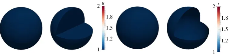
Figure 2.Numerical solutions corresponding to the coupled system of BSRDEs (2.1)–(2.5) withdΩ=1 in the bulk anddΓ=1 on the surface. The uniform steady-state solutions are converged to and no patterns form. Columns 1 and 2: solutions in the bulk
representingu. Columns 3 and 4: solutions on the surface representingr. Second and fourth columns represent cross sections of
the bulk and the surface, respectively. (Online version in colour.)
(i) Simulations of the coupled system of BSRDEs with (
d
Ω,
d
Γ)
=
(1, 1)
The bulk-surface finite-element numerical simulations of the coupled system of BSRDEs with dΩ=1 in the bulk,dΓ=1 on the surface are shown infigure 2. We observe that no patterns form in complete agreement with theoretical predictions. Similar to classical reaction–diffusion systems, diffusion coefficients must be greater than one. In particular, the diffusion coefficients must be greater than their corresponding respective critical diffusion coefficients in the bulk and on the surface. An example is shown next.
(ii) Simulations of the coupled system of BSRDEs with (
d
Ω,
d
Γ)
=
(1, 20)
For illustrative purposes, let us take dΩ=1 in the bulk, dΓ=20>dcritΓ =8.5 on the surface.
15
rspa.r
oy
alsociet
ypublishing
.or
g
Proc
.R
.Soc
.A
47
1
:2
[image:15.493.64.437.45.136.2]0140546
...
2.93
0.237
u
2
1
3.07
0.213
r
2 3
1
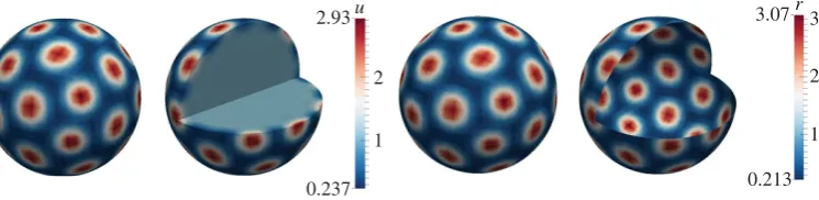
Figure 3.Numerical solutions corresponding to the coupled system of BSRDEs (2.1)–(2.5) withdΩ=1 in the bulk anddΓ=20
on the surface. Columns 1 and 2: solutions in the bulk representingu. Columns 3 and 4: solutions on the surface representingr.
Second and fourth columns represent cross sections of the bulk and the surface, respectively. Spot patterns form on the surface, whereas small balls form in the vicinity of the surface inside the bulk. (Online version in colour.)
0.146 3.99u
3
2
1
0.7
0.9r
0.88
0.84
0.80
0.76
0.72
Figure 4.Numerical solutions corresponding to the coupled system of BSRDEs (2.1)–(2.5) withdΩ=20 in the bulk and
dΓ=1 on the surface. Columns 1 and 2: solutions in the bulk representingu. Columns 3 and 4: solutions on the surface
representingr. Second and fourth columns represent cross sections of the bulk and the surface, respectively. Spectacular
patterning occurs in the bulk exhibiting spots, stripes and circular patterns. The surface dynamics produce uniform patterning. (Online version in colour.)
of the surface membrane. Spots are observed to form on the surface, whereas in the bulk, small balls form inside. Far away from the surface, no patterns form, because the necessary conditions for diffusion-driven instability are not fulfilled in the bulk. These results confirm our theoretical predictions. We note that this particular example describes realistically pattern formation in biological systems. We expect skin patterning to manifest in the epidermis layer as well as on the surface.
(iii) Simulations of the coupled system of BSRDEs with (
d
Ω,
d
Γ)
=
(20, 1)
To generate patterns in the bulk, we takedΩ=20>dcritΓ =8.5 anddΓ=1 on the surface.Figure 4
exhibits stripe, circular and spot patterns in the bulk as illustrated by the cross sections. On the surface, small amplitude patterns occur consistent with theoretical predictions. Although the patterns for theuspecies (columns one and two) appear uniform on the surface this is simply owing to the colour scale, with the amplitude of the patterns in the bulk larger than those on the surface. This difference in the amplitude of the pattern of the bulk solution in the bulk and on the surface is due to the Robin-type boundary conditions. Unlike zero-flux (also known as homogeneous Neumann), boundary conditions for standard reaction–diffusion systems which imply that no species enter or leave the domain, here, there is deposition or removal of chemical species through the flux on the surface, resulting in differences in amplitude between the bulk and surface solutions.
(iv) Simulations of the coupled system of BSRDEs with (
d
Ω,
d
Γ)
=
(20, 20)
16
rspa.r
oy
alsociet
ypublishing
.or
g
Proc
.R
.Soc
.A
47
1
:2
0140546
...
4
4.06 3.25
0.208 0.201
u r
3
3
2
1 2
1
Figure 5.Numerical solutions corresponding to the coupled system of BSRDEs (2.1)–(2.5) withdΩ=20 in the bulk anddΓ =
20 on the surface. Columns 1 and 2: solutions in the bulk representingu. Columns 3 and 4: solutions on the surface representingr.
Second and fourth columns represent cross sections of the bulk and the surface, respectively. We observe spot pattern formation both in the bulk and on the surface. (Online version in colour.)
the surface. In the bulk, we observe the formation of balls (which can be seen as spots through cross sections) and these translate to spots on the surface. The surface dynamics themselves induce spot pattern formation.
4. Conclusion, discussion and future research challenges
We have presented a coupled system of BSRDEs whereby the bulk and surface reaction–diffusion systems are coupled through Robin-type boundary conditions. Nonlinear reaction-kinetics are considered in the bulk and on the surface and for illustrative purposes, the activator-depleted model was selected because it has a unique positive steady state. By using linear stability theory close to the bifurcation point, we state and prove a generalization of the necessary conditions for Turing diffusion-driven instability for the coupled system of BSRDEs. Our most revealing result is that the bulk reaction–diffusion system has the capability of inducing patterning (under appropriate model and compatibility parameter values) for the surface reaction–diffusion model. On the other hand, the surface reaction–diffusion is not capable of inducing patterning everywhere in the bulk; patterns can be induced in only regions close to the surface membrane. For skin pattern formation, this example is consistent with the observation that patterns will form on the surface as well as within the epidermis layer close to the surface. We do not expect patterning to form everywhere in the body of the animals.
Our studies reveal the following observations and research questions still to be addressed:
— our numerical experiments reveal that the Robin-type boundary conditions seem to introduce a boundary layer coupling the bulk and surface dynamics. However, these boundary conditions do not appear explicitly in the conditions for diffusion-driven instability and this makes it difficult to theoretically analyse their role and implications to pattern formation. Further studies are required to understand the role of these boundary conditions as well as the size of the boundary layer;
— the compatibility condition (2.12) implies that the uniform steady state in the bulk is identical to the uniform state on the surface. We are currently studying the implications of relaxing the compatibility condition;
— finally, in this manuscript, we have not carried out detailed parameter search and estimation to deduce the necessary and sufficient conditions for pattern generation as well as isolating excitable wavenumbers in the bulk and on the surface. Such studies might reveal more interesting properties of the coupled bulk-surface model and this forms part of our current studies.
17
rspa.r
oy
alsociet
ypublishing
.or
g
Proc
.R
.Soc
.A
47
1
:2
0140546
...
developmental biology, tissue engineering and regenerative medicine and biopharmaceutical where reaction–diffusion-type models are routinely used [5,6,11–14,16,17].
We have restricted our studies to stationary volumes. In most cases, biological surfaces are known to evolve continuously with time. This introduces extra complexities to the modelling, analysis and simulation of coupled systems of BSRDEs. In order to consider evolving bulk-surface partial differential equations, evolution laws (geometrical) should be formulated describing how the bulk and surface evolve. Here, it is important to consider specific experimental settings that allow for detailed knowledge of properties (biomechanical) and processes (biochemical) involved in the bulk-surface evolution. Such a framework will allows us to study three-dimensional cell migration in the area of cell motility [16,27–29]. In future studies, we propose to develop a three-dimensional integrative model that couples bulk and surface dynamics during growth development or movement.
Data accessibility. This manuscript does not contain primary data and as a result has no supporting material associated with the results presented.
Acknowledgements. The authors thank anonymous reviewers for their constructive comments.
Funding statement. This work (A.M. and C.V.) is supported by the Engineering and Physical Sciences Research Council grant: (EP/J016780/1). A.M. and C.V. acknowledge support from the Leverhulme Trust Research Project Grant (RPG-2014-149). A.H.C. was supported partly by the University of Sussex and partly by the Medical Research Council.
Conflict of interests. The authors have no competing interest.
References
1. Bianco S, Tewes F, Tajber L, Caron V, Corrigan OI, Healy AM. 2013 Bulk, surface properties and water uptake mechanisms of salt/acid amorphous composite systems.Int. J. Pharm.456, 143–152. (doi:10.1016/j.ijpharm.2013.07.076)
2. Kwon Y, Derby JJ. 2001 Modeling the coupled effects of interfacial and bulk phenomena during solution crystal growth. J. Crystallogr. Growth 230, 328–335. ( doi:10.1016/S0022-0248(01)01345-8)
3. Medvedev ES, Stuchebrukhov AA. 2011 Proton diffusion along biological membranes.J. Phys. Condensed Matter23, 234103. (doi:10.1088/0953-8984/23/23/234103)
4. Levine H, Rappel WJ. 2005 Membrane-bound Turing patterns.Phys. Rev. E72, 061912. 5. Rätz A, Röger M. 2012 Turing instabilities in a mathematical model for signaling networks.
J. Math. Biol.65, 1215–1244. (doi:10.1007/s00285-011-0495-4)
6. Rätz A, Röger M. 2013 Symmetry breaking in a bulk-surface reaction–diffusion model for signaling networks. (http://arxiv.org/abs/1305.6172v1)
7. Turing AM. 1952 The chemical basis of morphogenesis.Phil. Trans. R. Soc. Lond. B237, 37–72. (doi:10.1098/rstb.1952.0012)
8. Gierer A, Meinhardt H. 1972 A theory of biological pattern formation.Kybernetik12, 30–39. (doi:10.1007/BF00289234)
9. Murray JD 2003Mathematical biology II: spatial models and biomedical applications, 3rd edn. Berlin, Germany: Springer.
10. Elliott CM, Ranner T. 2012 Finite element analysis for a coupled bulk-surface partial differential equation.IMA J. Numer. Anal.33, 377–402. (doi:10.1093/imanum/drs022) 11. Novak IL, Gao F, Choi Y-S, Resasco D, Schaff JC, Slepchenko BM. 2007 Diffusion on a curved
surface coupled to diffusion in the volume: application to cell biology.J. Comp. Phys.226, 1271–1290. (doi:10.1016/j.jcp.2007.05.025)
12. Chechkin AV, Zaid IM, Lomholt MA, Sokolov IM, Metzler R. 2012 Bulk-mediated diffusion on a planar surface: full solution.Phys. Rev. E86, 041101.
13. Nisbet DR, Rodda AE, Finkelstein DI, Horne MK, Forsythe JS, Shen W. 2009 Surface and bulk characterisation of electrospun membranes: problems and improvements.Colloids Surf. B, Biointerfaces71, 1–12. (doi:10.1016/j.colsurfb.2009.01.022)
14. Medvedev ES, Stuchebrukhov AA. 2013 Mechanism of long-range proton translocation along biological membranes.FEBS Lett.587, 345–349. (doi:10.1016/j.febslet.2012.12.010)
18
rspa.r
oy
alsociet
ypublishing
.or
g
Proc
.R
.Soc
.A
47
1
:2
0140546
...
16. Elliott CM, Stinner B, Venkataraman C. 2013 Modelling cell motility and chemotaxis with evolving surface finite elements.J. R. Soc. Interface9, 3027–3044. (doi:10.1098/rsif.2012.0276) 17. Venkataraman C, Sekimura T, Gaffney EA, Maini PK, Madzvamuse A. 2011 Modeling
parr-mark pattern formation during the early development of Amago trout.Phys. Rev. E84, 041923. (doi:10.1103/PhysRevE.84.041923)
18. Dziuk G, Elliott CM. 2007 Surface finite elements for parabolic equations.J. Comp. Math.25, 385–407.
19. Madzvamuse A, Chung AHW. Submitted The bulk-surface finite element method for reaction–diffusion systems on stationary volumes.SIAM SISC.
20. Bangerth W, Heister T, Heltai L, Kanschat G, Kronbichler M, Maier M, Turcksin B, Young TD. 2013 Thedeal.IIlibrary, version 8.1arXiv preprint.
21. Macdonald CB, Merrimanb B, Ruuth SJ. 2013 Simple computation of reaction–diffusion processes on point clouds. Proc. Natl Acad. Sci. USA 110, 9209–9214. (doi:10.1073/ pnas.1221408110)
22. Lakkis O, Madzvamuse A, Venkataraman C. 2013 Implicit–explicit timestepping with finite element approximation of reaction–diffusion systems on evolving domains.SINUM51, 2309– 2330. (doi:10.1137/120880112)
23. Prigogine I, Lefever R. 1968 Symmetry breaking instabilities in dissipative systems. II.J. Chem. Phys.48, 1695–1700. (doi:10.1063/1.1668896)
24. Schnakenberg J. 1979 Simple chemical reaction systems with limit cycle behaviour.J. Theor. Biol.81, 389–400. (doi:10.1016/0022-5193(79)90042-0)
25. Venkataraman C, Lakkis O, Madzvamuse A. 2012 Global existence for semilinear reaction– diffusion systems on evolving domains.J. Math. Biol. 64, 41–67. ( doi:10.1007/s00285-011-0404-x)
26. Madzvamuse A, Chung AHW. 2014 Fully implicit time-stepping schemes and non-linear solvers for systems of reaction–diffusion equations.Appl. Math. Comp.244, 361–374. (doi:10.1016/j.amc.2014.07.004)
27. George UZ, Stephanou A, Madzvamuse A. 2013 Mathematical modelling and numerical simulations of actin dynamics in the eukaryotic cell. J. Math. Biol. 66, 547–593. (doi:10.1007/s00285-012-0521-1)
28. Madzvamuse A, George UZ. 2013 The moving grid finite element method applied to cell movement and deformation. Finite Element Anal. Des. 74, 76–92. (doi:10.1016/j.finel. 2013.06.002)