Mechanisms of Proton Proton Inelastic Cross Section Growth in Multi Peripheral Model within the Framework of Perturbation Theory Part 1

Mechanisms of Proton-Proton Inelastic Cross-Section

Growth in Multi-Peripheral Model within the

Framework of Perturbation Theory. Part 1

Igor Sharf1_{, Andrii Tykhonov}1,2_{, Grygorii Sokhrannyi}1_{, Maksym Deliyergiyev}1,2_,

Natalia Podolyan1_{, Vitaliy Rusov}1,3*

1_{Department of Theoretical and Experimental Nuclear Physics,}

Odessa National Polytechnic University, Odessa, Ukraine

2_{Department of Experimental Particle Physics, Jožef Stefan Institute, Ljubljana, Slovenia} 3_{Department of Mathematics, Bielefeld University, Bielefeld, Germany}

E-mail:*_{siiis@te.net.ua}

Received July 28, 2011; revised September 30, 2011; accepted October 22, 2011

Abstract

We demonstrate a possibility of computation of inelastic scattering cross-section in a multi-peripheral model by application of the Laplace method to multidimensional integral over the domain of physical process. Founded the constrained maximum point of scattering cross-section integral under condition of the energy-momentum conservation. The integrand is substituted for an expression of Gaussian type in the neighborhood of this point. It made possible to compute this integral numerically. The paper has two parts. The hunting procedure of the constrained maximum point is considered and the properties of this maximum point are discussed in the given part of the paper. It is shown that virtuality of all internal lines of the “comb” diagram reduced at the constrained maximum point with energy growth. In the second part of the paper we give some the argu- ments in favor of consideration of the mechanism of virtuality reduction as the mechanism of the total had- ron scattering cross-section growth, which is not taken into account within the framework of Regge theory.

Keywords:Inelastic Scattering Cross-Section, Total Scattering Cross-Section, Laplace Method, Virtuality, Multi-Peripheral Model, Regge Theory

1. Introduction

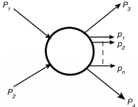
[image:1.595.356.492.595.701.2]

Despite the fact the multi-peripheral model [1] has been used for description of hadron scattering for a long time, formal difficulties, which appear in calculating of inelas- tic scattering cross-section, in our opinion, are not over- came until now. These difficulties are caused by the fact that inelastic scattering cross-section with production of a given number of secondary particles in the finite state

Figure 1 is described by the multidimensional integral of scattering amplitude squared modulus over the phase volume of finite state:

 

 

 

 

3 4

3 3 3

1

30 40 0

4

3 4 1 2

1

d d d

1

4 ! _{2 2π 2 2π 2 2π}

n k n

k _k

n k k

n I _{P P p}

P P p P P











 

  _     _

 







P P p

(1)

with



 

2



2

1 2 1 2

I P P  M M (2a)





2

1 2 1 2 3 4

, , , , n, , , ,

T n p p p P P P P

   (2b)

where M₁ and M₂ are the masses of colliding parti-

cles with four-momentums P1 and P2;



, ,1 2, , n, , , ,1 2 3 4



T n p p  p P P P P is scattering amplitude corresponding to inelastic process shown in Figure 1;

(4)

 is a four-dimensional delta function describing the conservation laws of energy and three momentum com-ponents in this process. Here it is also assumed that par-ticles with four-momentums P₃ and P₄ are the same sorts as P1 and P2, respectively, and n seconddary

particles with four-momentums p p1, 2, , pn are

iden-tical. Since scattering amplitude is, in general, not a product of functions of some variables, and also due to the complexity of integration domain, the multidimen- sional integral in Equation (1) is not a product of small-er-dimensional ones. In considered inelastic process this domain of phase space of finite state particles is deter-mined by the energy-momentum conservation law. As a result, the integration limits for one variable depend on the values of others. In order to overcome these difficult- ties one usually deals with the multi-Regge kinematics [2-10].

In our approach we will adopt well-known Laplace method [11] for scattering amplitude, which represented by set of multi-peripheral diagrams Figure 2 within the framework of the perturbation theory in order to over- come these difficulties. The essence of this method con- sists in finding the constrained maximum point of scat- tering amplitude squared modulus in Equation (1) under four conditions imposed by _(4)_{-function of Equation}

(1). Then, expressing the scattering amplitude squared modulus as T2 exp ln



 

T2



, it is possible to expand the exponent in Taylor series in the neighborhood of constrained maximum point, coming to nothing more than quadratic items. After that we obtain Gaussian inte- gral, whose calculation is reduced to computation of ma- trix determinant of second derivatives with respect to

 

2

[image:2.595.311.542.186.453.2]

ln T . Now let us consider solution of the listed above problems step by step.

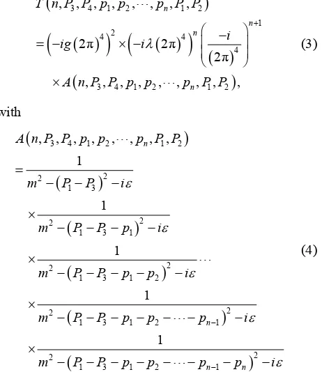
Figure 2.An elementary inelastic scattering diagram in the multi-peripheral model (“the comb”).

2. Consideration of the Scattering Amplitude

Symmetry Properties

At first we examine some simplifications, which is pos- sible to make before hunting for the solution of con- strained maximum problem. According to Feynman dia- gram technique, the expression for scattering amplitude, which corresponds to a diagram Figure 2 has form:





 







 



 





3 4 1 2 1 2

1 2

4 4

4

3 4 1 2 1 2

, , , , , , , ,

2π 2π

2π

, , , , , , , , ,

n

n n

n T n P P p p p P P

i

ig i

A n P P p p p P P





 _ 

 

   

 

 







(3)

with

























3 4 1 2 1 2

2 2

1 3

2 2

1 3 1

2 2

1 3 1 2

2 2

1 3 1 2 1

2 2

1 3 1 2 1

, , , , , , , , 1

1

1

1

1

n

n

n n

A n P P p p p P P

m P P i

m P P p i

m P P p p i

m P P p p p i

m P P p p p p i

















  



   



    



      



       









(4)

where g is a coupling constant in the outermost verti- ces of the diagram;  is a coupling constant in all other vertices; m is the mass of virtual particle field and also secondary particles. As in the original version of multi- peripheral model [1], pions are taken both as virtual and secondary particles. It was assumed that the particle masses with four-momentums P1, P2, P3, P4 are

equal, i.e., M1M2M3M4M . The proton mass

was taken as M. Note that the concrete choice of nu- merical value of mass M has no importance for the re- sults presented in the paper.

As it was noted in [2], for the most ratios of particle masses in the initial and final state, the virtual particles four-momentums on the diagram of Figure 2 are space- like, i.e., their scalar squares are negative in Minkowski space. The negativity of scalar squares of virtual four- momentums at the given mass configuration

1 2 3 4

M M M M M is easy to prove (see Appen- dix A).

Since the virtual particle squared four-mometum





2

1 3

are negative at the physical values of four-momentums of particles in the finite state, denominators in Equation (1) do not equal to zero nowhere in the physical region. Therefore it is possible to reduce i to zero before all calculations.

Due to negativity of virtual particle squared four- momentums the magnitude Equation (4) is real and positive. Therefore the search of the constrained maxi- mum point of scattering amplitude squared modulus reduces to the search of the constrained maximum point of function Equation (4). Hereinafter we’ll refer the expression Equation (4) as well as Equation (3), which differs from it by constant factor, as scattering ampli-tude, for short.

Let us examine Equation (4) in c.m.s. of colliding par- ticles P1 and P2. In such a frame of reference the ini-

tial and finite states have some symmetry, which is pos- sible to use for solving the constrained maximum prob- lem. In particular, the consideration of symmetries makes it possible to reduce the search of the constrained maxi- mum of scattering amplitude to the search of the maxi- mum of its restriction on a certain subset of physical process domain shown in Figure 2. This restriction is the function of substantially smaller number of independent variables than the initial amplitude.

For the further discussion of these symmetries and re- lated simplifications, it would be convenient at first to take into account the conservation laws, expressing the scattering amplitude as a function of independent vari- ables only. After decomposition of the three-dimensional particle momentums in c.m.s. frame to components, which are parallel p_k|| and orthogonal k_k to collision axis, and lets name them longitudinal and transversal momentums, respectively.

Energy of each particles in the finite state can be ex- pressed by their momentum using the mass shell condi- tions, having n2 particles in finite state Figure 2, that give us 3(n2) momentum components of these particles. Since we are looking for a constrained extre- mum, it is necessary to take into account four relations, which express an energy-momentum conservation law. It will result in the fact that amplitude Equation (4) can be represented as a function of 3n2 independent vari- ables. The first 3n variables we choose are longitudinal and transverse components of momentums p p1, 2, , pn,

of particles produced along the “comb“ in Figure 2. The other two variables are the transverse components of momentum P3.

If z-axis coincides with momentum direction P1 in

c.m.s. and x and y axes are the coordinate axes in the plane of transverse momentums, the conservation laws look like

















30 40 10 20 0

3|| 4|| 1|| 2|| ||

4 1 2 3

4 1 2 4

n n

x x x n x x

y y y n y y

P P s p p p

P P p p p

P p p p P

P p p p P

    

    

     

     

     

     









(5)

with





 









 





 

 





 

2 1 2

2

2 2

2

0 ||

2

2 2

2

30 3||| 3 3

2

2 2

2

40 4|| 4 4

k k k x k y

x y

x y

s P P

p m p p p

p M P P P

P M P P P

 

 

 

 

   

   

   

(6)

Let’s enter the following denotations:

















10 20 0

|| 1|| 2|| ||

1 2

1 2

p n

p n

px x x n x

py y y n y

E s p p p

P p p p

P p p p

P p p p

  

  

    

    

    

    









(7)

Then solving the system Equation (5) for the unknown

3||

P , P4||, P4x, P4y, we have:

 





 





2 2

3

3 || 2

2 2

3

4 || 2

4 1 2

4 1 2

b a

p p

b a

b a

p p

b a

M E

E

P P E

E E

M E

E

P P E

E E





 _ 

 

 _   _

 

 

 _ 

 

 _  _

 

 



 

P

P

(8)

where



,



p Ppx Ppy

P (9a)





2 2 2

|| 2 3

a p p p p

E E P P_ P_P_ (9b)



2 2



||

b p p

E  E P (9c)

We will discuss the choice of sign in Equation (8) fur- ther in the paper. Note that the value of P3 will not

change, if we change the signs of all transversal momen- tums in Equation (8) simultaneously.

Substituting P3 from Equation (8) to Equation (6),

and resulting P30 from Equation (6) into Equation (4),

Taking into account this fact, we can define the ampli- tude Equation (4) as



, 3 , 1 , 2 , , n , 1||, 2||,..., n||



A n P p p  p p p p (10) enumerating only independent variables in the argument list. When the scattering amplitude will be expressed in terms of independent variables only, it is possible to find the ordinary extremum, but not constrained extremum.

Now let us examine symmetries of the scattering am- plitude in c.m.s. Obviously, the system has a symmetry under rotations around the collision axis, it means that there is no preferred direction in the plane orthogonal to collision axis. Hence, if the scattering amplitude has the constrained maximum point, it must be achieved at zero values of the particle momentums components in finite state transversal to collision axis. Otherwise these mo- mentums must be somehow directed in the plane of transversal momentums, while all directions are equiva- lent in this plane.

To show more formally previous conclusion we use an explicit form of amplitude Equation (4), which trans- forms to itself, when the signs in front of all transversal momentums are changed:









3 1 2 1|| 2|| ||

3 1 2 1|| 2|| ||

, , , , , , , ,...,

, , , ,..., , , ,...,

n n

n n

A n p p p

A n p p p

   

   

    



P p p p

P p p p

(11)

Take derivative from Equation (11) with respect to any of transversal momentum arguments and after that assuming all transversal momentums equal to zero, we obtain that all partial derivatives with respect to trans- verse momentum arguments are equal to zero if this ar- guments are equal to zero.

Thus, for the further search of the constrained maxi- mum we can limit ourselves to reduction of the scattering amplitude on a subset of the values of its independent arguments, which corresponds to zero values of trans- versal momentums of all particles in finite state. This reduction is a function of longitudinal components of momentum p p1, 2, , pn which we designate as





|| , 1||, 2||, , n||

A n p p  p and from Equation (4) we get:





















1 2

1 ₁

2 2

2 2 2 2

10 30 1 3

1

, , , , _n

n

l l i

A n p p p

m P P P P  m   



     



 

   

 



(12) where

10 30 0

1

l

l k

k

P P p





  



(13a)

1|| 3|| || 1

l

l k

k

P P p





  



(13b)

 

2 2

0 ||

k k

p  m  p (13c)

 

2 2 30 3||

P  M  P (13d)

At the same time, assuming that all transversal mo- mentums equal to zero, we have from Equation (8):

   

   

2

3 || 2 2

|| 2

4 || 2 2

||

1 4

1 2

1 ₁ 4

2

p p

p p p p

p p

M

P P E

E P

M

P P E

E P

 

 

 _   _

  

 

 

 

 _  _

  

 



 

(14)

Moreover, we have in c.m.s. P₁₀ s 2 and

2 1|| 4

P  s M , where s is determined in Equation (6). For the further analysis it is convenient to switch from longitudinal momentums of secondary particles to rapid- ities yk, defined by following relation:

 

|| , 1, 2, ,

k k

p  m sh y k  n. (15) The function A || can be written as





|| , 1||, 2||, , n||

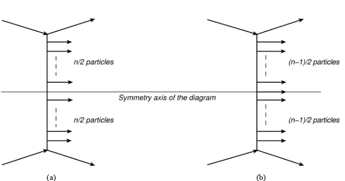
A n y y  y . The initial state in c.m.s is sym- metric with respect to changes in positive direction of collision axis. In addition, those type of diagrams of pre- sented in Figure 2 have an axis of symmetry shown in

Figure 3 for the case of even number Figure 3(a) and for the case of odd number Figure 3(b) of secondary particles.

From the explicit expression for amplitude Equation (12) can be shown that this expression will transform to itself, if we place instead the rapidity of every particle, the rapidity of particle symmetrically arrangement along the axis of symmetry Figure 3 and at the same time change the rapidity sign. Other words, if we change the variables for even number of particles

1 2 1 ₁

2 2

1 1

2 2

, , , ,

, ,

n n n n

n n n

y y y y y y

y y y y

 _



     

   



 (16)

the expression of restriction amplitude





|| , 1||, 2||, , n||

A n y y  y will transform to itself. In case of odd number of particles the transformation similar to Equation (16), but instead of the rapidity y_{n1 /2 1 }

which forms the axis of symmetry in Figure 3, must be substituted y_{n1 /2 1 } into the expression for the am-plitude. The examined features of function





|| , 1||, 2||, , n||

A n y y  y can be expressed in the following symmetry relations for even number n of secondary particles:

[image:5.595.131.468.66.243.2]

(a) (b)

Figure 3.An elementary inelastic scattering diagram in the multi-peripheral model with even (a) and with odd (b) number of particles on the “comb” and it symmetry axis.

|| 1 2 ₁ || 1 ₁ 1

2 2 2 2

, , , , _n, _n , , _n , _n, _n , , _n , _n, ,

A n y y y y _ y A n y y y _ y y

   

     

   

   

        (17)

and for odd number of secondary particles n, respectively

|| 1 2 1 1 1 1 || 1 1 1 1 2 1

1 2 2 1

2 2 2 2 2 2

, , , n , n , n , , n , n , n, n , , n , n , n , , ,

A n y y y y _ y _ y y A n y y y _ y _ y y y

   

       

   

   

        (18)

Proof of symmetry relations Equation (17) is given in Appendix B.

Now let us switch to new variables for even number of n.

1

1 2 1 1 2 2

1 2

2

1

1 2 1 1 2 2

1 2

2

, , , , ,

2 2 2 2

, , , , ,

2 2 2 2

n n

n n k n k

k n

n n

n n k n k

k n

y y

y y y y y y

y y y y

y y

y y y y y y

y y y y



      



      



  

   



  

   

 

 

(19)

and for odd number of n

1 1

2

1 2 1 1 2 2

1 2 1 1 ₁ 1 ₁

2 2 2

1 1

2

1 2 1 1 2 2

1 2 1

2

, , , , , ,

2 2 2 2

, , , , ,

2 2 2 2

n n

n n k n k

k n n n

n n

n n k n k

k n

y y

y y y y y y

y y y y y y

y y

y y y y y y

y y y y

 _

       

 _ _

 _

      





  

    



  

   

 

 

(20)

In these variables, the symmetry relation Equation (17) becomes

|| 1 2 1 2 ₁ || 1 2 1 2 ₁

2 2 2 2 2 2

, , , , n, , , , n , n , , , , n, , , , n , n

A n y y  y y y   y y A n y y y y y   y y

 

   

   

   

   

        (21)

and relation Equation (18) becomes

1 2 1 1₁ 1 2 1 1 2 1 1₁ 1 2 1

2 2 2 2 2 2

, , , , n , n , , , , n , , , , n , n , , , , n

A n y y  y y_ y y  y A n y y y y_ y y  y

   

    

   

   

   

Computing step by step the partial derivative of func- tion Equation (21) with respect to variables y1

_,

2

y, ···,

/ 2

n

y , we obtain

1 2 1 2

1

2 2 2

1 2 1 2

1

2 2 2

, , , , , , , , ,

, , , , , , , , ,

n n n

k

n n n

k

A n y y y y y y y

y

A n y y y y y y y

y

      

 _

      

 _

 



 

 

 _{ }

 



  _    _

 _{ }

 

 

 

(23)

where k1, 2, , 2 n .

It follows from relation Equation (23) for zero values of yk

 _{the derivatives of the function}





|| , 1, 2, , n/ 2, 1, 2, , ( /2) 1n , n/2

A n y y   y y y   y  y

vanish. In the same way it can be shown that in case of odd number n of particles that for zero values of yk the derivatives of scattering amplitude

 

   





|| , 1, 2, , n 1 / 2 1, 1, 2, , n 1 / 2

A n y y  y y y  y 

 

 

also vanishes.

This shows that for the extremumsearch we can con- sider a further reductionof the scattering amplitude on a subsetof zero values of variables y_k_{. By virtueof}

Equ-ations (20)-(21) on this subset we have y_k _y_{k ,}





1, 2, , 1 2

k  n at even n and y_k_ y_k,

1, 2, , 2

k  n at odd n.Designating this reduction as

0

A we obtainat even n:





   





0 1 2 /2

1 2 /2 1 /2 /2 1 2 1 , , , ,

, , , , , , , , ,

n n

n n

A n y y y

A n y y y _ y y _ y y



  





  (24)

and at odd n

 





 

       





0 1 2 1 /2

1 2 1 /2 1 1 / 2 1 1 /2 1 , , , ,

, , , , 0, , ,

n

n n n

A n y y y

A n y y y y y y



    



   







(25) If we now examine the formula Equation (12) on sub- set, where reduction A0 is considered, we will have

0

p

P  by virtue of Equation (7). And therefore instead of Equation (14) we have the following expressions:

 

 

2 2

3|| 2 4|| 2

4 4

1 , 1

2 2

p p

p p

E M E M

P P

E E



    (26)

or

 

 

2 2

3|| 2 4|| 2

4 4

1 , 1

2 2

p p

p p

E M E M

P P

E E



    (27)

Let us take into account that if we decompose all sca- lar square terms in denominators of Equation (4) they

will include the following difference

2

1|| 3|| 4 3||

P P  s M P and negative Equation (27), chosen as the P 3|| in the end will give us greater value

in the denominator than in the choice of Equation (26). Therefore it is naturally to suppose that the main contri- bution to cross-section Equation (1) gives the range of constrained maximum point determined by the scattering amplitude, where P3|| and P4|| are given by Equation

(26), but not by Equation (27). Hence, considering the expression Equations (24) and (25) for the reduction of the scattering amplitude at zero transverse momentum region, and performing further transformations, we assume that

3||

P and related with it 2

 

2 30| 3||

P  M  P are ex-pressed in terms of the longitudinal momenta of secon-dary particles by the relation Equation (26).

After we move on to the appropriate amplitude reduc- tion A0 both in case of diagrams with even and odd

number of particles we obtain function of particles rapid- ities located above the axis of symmetry in the diagram. The considered features of symmetry make it possible to simplify the energy parametrization of virtual particles, to which correspond the transversal lines located above axis of symmetry of diagrams in Figure 3.

Applying symmetry relation and conversation of en- ergy, it follows that on subset, on which the considered amplitude reduction A0 is defined, the energy corre-

sponding to the line connecting n 2 and n 2 1 ver- tices of the diagram in Figure 2 is equal to zero in case of even number of particles at any values of independent variables (on which A0 depends). Similarly, for an odd

number of particles the energy transferred along the line, which joins



n1 2



and



n1 2 1



 vertices, is equal to m 2. The corresponding proof is given in Ap- pendix C.

Taking into account these results, reduction of A0 for

the diagram in Figure 2 with even number of particles can be written in the form, which is convenient for the further numerical and analytical calculations:

 

2 2

2 ₂

2 0 1 2

1 2

2

2 2 1

2 2

2

|| 1 2

1 2 2 2

|| 1 , , , ,

n

n k M

k

n n

j

k M k

k j k

j

n

M k

k

A n y y y m E S

m E S p

m S p





 

 







 _{ } 

   _{ } 

  

   

  _ _

   _{ } 

 

 _{ }



 _{ }   _

 _ _{ } _  _



 

 

 _{ } 



 _{ } 

 _{ } 

_ _  _{ }

 

 _{ } 

 













where

2 3||

4

M

S  s M P (29a)

 

k k

E  m ch y (29b)

 

||

k k

p  m sh y (29c) The similar expression in case of odd number of parti- cles in comb looks like:

 

2 2

1

2 ₂

2 0 1 2 1

1 2

2

1 1 ₂ 2

1

2 2

2

|| 1 2

1 2 1

2 ₂

2

|| 1 , , , ,

2

2

2

n

n k M

k

n n

j

k M k

k j k

j

n

M k

k m

A n y y y m E S

m

m E S p

m

m S p

 





  



 



 



 _{ } 

   _{ } 

   

   

  _ _

   _{ } 

 

 _{ }



 _{ }  

  _ _  _ _  _



 

 

 _{  }



 _{ } 

 _{   }  _ _{ } _  _{ }

  _{ }

 _{ } 

 













(30) As it follows from Equations (28)-(30), it is conven- ient for the further calculations to make all quantities dimensionless by mass m. In dimensionless form, these relations were used for numerical and analytical solution of the extremum for the reduction of the scattering am- plitude A₀.

3. Numerical Solving the Constrained

Maximum Problem for Multi-Peripheral

Scattering Amplitude Squared Module

Numerical solution of the constrained extremum problem was done using Mathcad 2001 [12,13]. As it was shown in the previous section, since scattering amplitude corre-sponding to Figure 2 is real and positive, we can search for amplitude maximum instead the maximum of ampli-tude squared module. For cases of low values of secon-dary particles n we search not for the maximum of reduction A0, but for the maximum of total amplitude A defined by Equation (4) with allowance for Equation (14) with the choice of positive sign in the front of P 3||

(in order to transform this expression to Equation (26), when the symmetry properties will be taken into ac-count). These calculations are numerical verification of validity of the discussed above simplifications related to the symmetry properties. A typical result of such calcu-lation for the case of n12 and energy s55 GeV using Maximize function of Mathcad 2001 is shown in

Table 1. As it follows from Table 1, the numerical

Table 1. A typical output of numerical computation of the maximum point of scattering amplitude corresponding to the diagram presented in Figure 2.

index y px py P3x P3y

1 3.33917 0 0 0 0

2 2.75454 0 0 - -

3 2.15274 0 0 - -

4 1.54160 0 0 - -

5 0.92590 0 0 - -

6 0.30901 0 0 - -

7 −0.30901 0 0 - -

8 −0.92590 0 0 - -

9 −1.54160 0 0 - -

10 −2.15274 0 0 - -

11 −2.75454 0 0 - -

12 −3.33917 0 0 - -

computation confirms above conclusion that all the trans- verse momentums must vanish at the maximum point. Note also that the set of rapidities corresponding to the maximum point in Table 1, which are determined by numerical computation, confirms conclusion that the dia- grams centered at the axis of symmetry have mutually opposite values in the point of rapidity extremum. Simi- lar results were obtained for different numbers of parti-cles n and energies s.

Now let us examine properties of the constrained maximum point following from the results of numerical computations. Some typical results are shown on Figure 5 and corresponding to it Table 2.

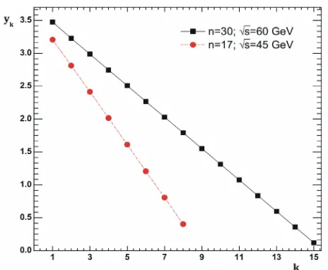
The column y in Figure 5 contains the rapidities of particles obtained using Maximize procedure (Mathcad) for which scattering amplitude A0 defined by Equation

(28) in the case of even number particles and by Equa- tion (30) in the case of odd number particles has maxi- mum reduction. Moreover, note that the order of num- bers in the columns match to the order of arguments in the corresponding function.

For instance, in Figure 4 at n30 the reduction de- termined by Equation (28) is the function of 15-teen va-riables A n0



15, , , ,y y1 2  y15



corresponding to the

particles rapidities joined to the upper 15-en vertices of the diagram in Figure 2. The column shown in Table 2

contains fifteen numbers, in which the function





0 15, , , ,1 2 15

A n y y  y has a maximum and at the same time the first number in the column is the value of

1

y, the second number is the value of y2 etc.

[image:8.595.57.289.76.267.2] [image:8.595.311.536.170.634.2]

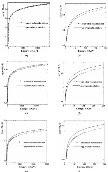
Figure 4. Rapidity dependence on vertex number in the diagram Figure 2 at the constrained maximum point.

(a)

(b)

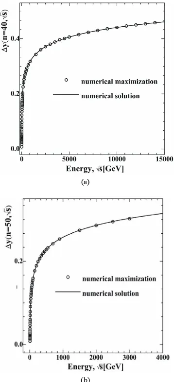
Figure 5. The dependence of rapidity step Δy of an arith-

metic progression, which constrainedly maximizing the scattering amplitude, on energy s for the different num-

bers n of particles on “the comb”. At high energies this de-

pendence become logarithmic.

Table 2. Resulting rapidities obtained using Maximize pro- cedure (Mathcad) for which scattering amplitude A0 de-

fined by Equation (28) in the case of even number particles and by Equation (30) in the case of odd number particles has maximum reduction. The column Δy contains a differ- ence between every column element and the successor of this column. The last column contains ratios yk/y15, k =

1 ,2, ···, 15 and yk/y8, k = 1 ,2, ···, 8.

Figure 4, n = 30 s = 60 GeV

index yk ∆y = yk –yk+1 yk/y15

1 3.475 0.2461 29.07

2 3.229 0.2417 27.01

3 2.987 0.2399 24.99

4 2.747 0.2392 22.98

5 2.508 0.2389 20.98

6 2.269 0.2387 18.98

7 2.03 0.2387 16.98

8 1.792 0.2387 14.99

9 1.553 0.2387 12.99

10 1.314 0.2388 10.99

11 1.075 0.2389 8.997

12 0.8365 0.2389 6.998

13 0.5976 0.239 4.999

14 0.3586 0.2391 3

15 0.1195 - 1

Figure 4, n = 17 s = 45 GeV

index yk ∆y = yk – yk+1 yk/y8

1 3.207 0.3929 7.951

2 2.814 0.3972 6.977

3 2.416 0.4016 5.992

4 2.015 0.4017 4.996

5 1.613 0.4061 4

6 1.207 0.3392 2.993

7 0.8079 0.4046 2.003

8 0.4033 - 1

[image:8.595.68.276.305.656.2]

In addition, the proximity of the sequence of yk

column elements to an arithmetic progression follows also from calculations of yk y8 and yk y15 columns,

which are constructed by the following principle. If we assume that yk form an arithmetic progression with

difference y , in the case of even n we obtain

/ 2 1 / 2

n n

y _ y  y. On the other hand, from symmetry

relations obtained in Section 2 we have yn/ 2 1  yn/ 2.

From these two relations we obtain yn/ 2  y 2. Then / 2 1 / 2 3 2 3 / 2

n n n

y _ y    y y  y and in the similar

manner yn/ 2 2 yn/ 2   2 y 5 y 2 5 yn/ 2, etc. Hence,

in case of the diagram with even n the rapidity ratios

/ 2 1 / 2, / 2 2 / 2, , 1 / 2

n n n n n

y _ y y _ y  y y must form the se-

quence of odd whole numbers. The columns yk y8 and 15

k

y y contains these ratios constructed by the column

elements yk obtained with the help of Maximize func-

tion [12]. As seen from Table 2, the column elements

8

k

y y and y_k y₁₅are really close to odd numbers.

In case of odd n with allowance for y_{n1 / 2 1 } 0

we have

1 1

1

2 2

1 ₁ 1

2 2

2

n n

n n

y y y y

y y y y

 _

_ 

    

     (31)

Then the ratios yn_{1/ 2} yn_{1/ 2}, yn1 / 2 1  yn1/ 2,

n1 / 2 2 n1/ 2,

y _{ } y_ must produce the sequence of whole

numbers 1,2, ···. And Table 1, where columns yk y₈

and yk y₁₅ consist of such ratios, shows that these

ratios are really close to the corresponding whole num- bers. The similar results are obtained for different num- bers of particles n and energies s.

The analytic form of arithmetic progression at any n

and s will be considered in more detail below the

text, when we will given an analytical solution of the extremum problem for reductions Equations (28) and (30).

Moreover, the results of numerical computations con- firm the well-known multi-peripheral model assumption about particle rapidity ordering, because at the maximum point the particle rapidities monotone increase at move- ment upward along the diagram in Figure 2.

Besides of these results numerical computation allows to trace several other properties of the extremum point. In particular, if the rapidities in the maximum point form an arithmetic progression, the question arises, how the difference y of this arithmetic progression depends

on the energy s and the number of particles n? Re-

sult of numerical computation of the dependence of dif- ference of an arithmetic progression y on s at

different numbers of particles on the “comb” Figure 2

are shown in Figure 5. At the same time the arithmetical average of column elements y (the similar to shown

in Table 2) was used as the value of y.

As it’s obvious from Figure 5, the y is a mono-

tonically increasing function of energy s for a fixed

number n of particles. At the same time the depend-

ence  y



s n, const



has some energy threshold.

It is obvious, that at given n such dependence makes

sense only at

2

snm M (32)

(where s is not dimensionless by m), that corre-

sponds to the total rest energy of particle in finite state. Note that function y

 

s reaches asymptotic quite

quickly. Since Figure 5 has a logarithmic scale on the energy axis, its seen that this asymptotic behavior is characterized by the linear dependence on logarithm of energy normalized to 1 GeV.

Output computation of the dependence of difference of an arithmetic progression y on the number of parti-

cles for set of energies s= 10 GeV, 100 GeV, 1000

GeV is presented in Figure 6. From Figure 6 (where dependences y n

 

are given in linear and logarithmic

scales) it is evident that, when n is small in comparison

with the boundary value determined by Equation (32), this dependence is close to inversely. In particular, if we examine ln

 

y as a function of ln

 

n , it is possible

to calculate corresponding difference of an arithmetic progressions for the given energy (they are marked as

1, 2, , k

y y y

    in Figure 8). As it follows from Table

3, ratios

 





 

 

2

ln ln

ln ln 2

j

j

y y

n

  

 (33)

where j1, 2, , k are close to (−1), which suggests

that if we fix s and examine n



s2M



m, that

is much smaller value than the maximum allowable by

Table 3. The difference of rapidity Δy from Figure 6. From

these results it is evident that the dependence is close to inverse proportion.

s

10GeV 100GeV 1TeV

4 2

ln( ) ln( )

ln(4) ln(2)

y y

  

 −1.009 −1.005 −1.002

6 2

ln( ) ln( )

ln(6) ln(2)

y y

  

 −1.011 −1.006 −1.003

20 2

ln( ) ln( )

ln(20) ln(2)

y y

  

 −1.057 −1.011 −1.002

40 2

ln( ) ln( )

ln(40) ln(2)

y y

  

 −1.203 −1.02 −1.009

60 2

ln( ) ln( )

ln(60) ln(2)

y y

  

[image:10.595.56.288.78.227.2]

Figure 6. Dependence of difference Δyin an arithmetic pro-

ession, which constrainedly maximizing the inelastic scat-tering amplitude for the different number of particles n on

the “comb” at the fixed energies s: 10 GeV, 100 GeV

and1000 GeV.

law of conservation of energy for a given value s, then we have _{y n~} 1_.

More specific information about the dependence



,



y n s

  can be obtainedfrom analytical solution of the constrainedextremum problem for scattering ampli- tude, which will be considered in the next section.

However, the greatest interest is the dependence of the absolute values of virtualities on energy (i.e. the virtual particle squared four-momentums corresponding to the diagram in Figure 2, calculated at values of real particle four-momentums for which the scattering amplitude has a constrained maximum). Discussion of this problem leads us to possible mechanism of inelastic scattering cross-section growth with energy.

Let us designate the virtual particle four-momentums according to Figure 2:

   

 

1 2

1 3 1 3 1

1 1 3

1

, , ,

,

j j

l l

k P P k P P p

k P P  p



       





 (34)

The numbers of four-momentums are taken in brackets to distinguish them from the four-momentum compo- nents notation. For example, notation _k(0)0 _denotes

zero component of contra variant four-vector _k(0)_.

As was noted above, all the quantities were made di- mensionless by the mass m before calculations, there- fore we introduce the notation

( ) ( )j k j

q m

 (35)

At the same time the magnitude A, which is deter- mined by Equation (4) and coincident with scattering amplitude accurate within constant, can be written in

dimensionless form like:

 

1

1 ₂

( ) 1

1

n

j j

A q

 



 

 _  _

 



(36)

From numerical computation we know particles four- momentums in finite state, for which function A has constrained maximum. Therefore, with help of relations Equations (34) and (35) we can calculate four-momen- tums _q( )j _{and whereupon calculate the corresponding} dimensionless virtualities. Results of such calculation presented on Figures 7 and 9.

(a)

[image:10.595.314.533.222.618.2]

(b)

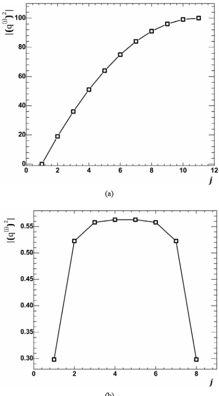
Figure 7. The virtuality variation along “the comb”. (a) shows particles virtuality dependence on vertex number on diagram Figure 2, for even number of particles (n = 20).

(a)

(b)

[image:11.595.312.539.67.275.2]

(c)

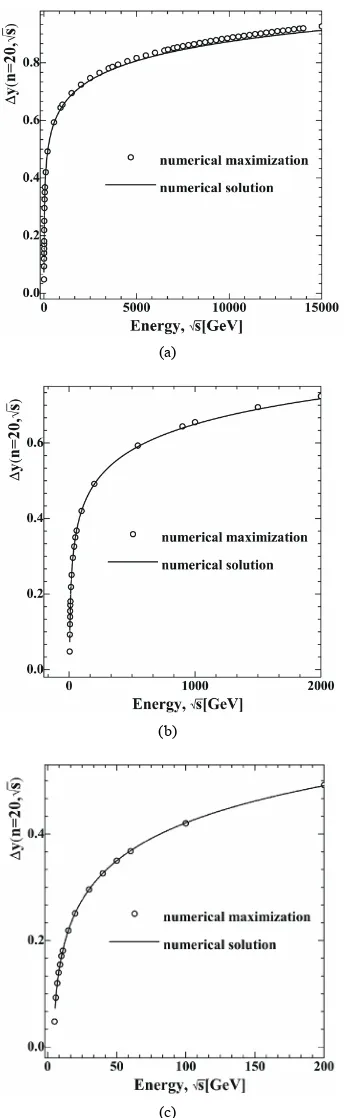
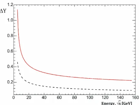
Figure 8. Comparison of the results of the numerical solu- tion of Equation (74) (solid line) with the results of numeri- cal maximization (circles) of the magnitude y



n, s



at n = 20 for the different energy ranges, GeV: 5 ÷ 16000 (8(a)); 5 ÷ 2000 (8(b)); 5 ÷ 200 (8(c)). Here, it is taken into

account that y



n, s



2yn/2.

Figure 9. Variation of the modulus of virtuality on energy for n = 20 at different energies.

As it well known, that there is reference frame where the particle energy vanishes [11] for particles with nega- tive virtuality. Such a reference frame is called the stan- dard reference system according to terminology of [11]. Obviously that the particle momentum in the standard reference system has the smallest possible value of all inertial frames of reference, and this smallest value is defined by particle’s virtuality.

Taking into account the Heisenberg uncertainty prin- ciple, we find that the virtuality characterizes a size of the domain, in which a particle can be detected with high accuracy, if the measurements were made in the standard reference system of this particle. At the same time, the more particle‘s virtuality, the smaller this size. Thus, the virtuality of particles makes it possible to judge the spa- tial extension of those domains, where inelastic proc- esses take place described by the diagrams of type Fig- ure 2. These space domains form the virtual “coats” of colliding particles, therefore these spatial extensions de- fine typical sizes of colliding particles P1 and P2, see Figure 2. From Figure 7 it is evident that virtualities increase with movement from the diagram edges to its center. This is easy to explain, because all the virtualities are negative and therefore

  

(1) 2 0 0



2





2

 

2 1 3 1|| 3|| 3 0

k  P P  P P  P  (37)

Taking into account that transversal components of momentum are equal to zero at the maximum point, we have:





2



_{0 0}



1|| 3|| 1 3

P P  P P (38)

[image:11.595.88.261.74.633.2]

have 0 0

3 1

P P . At the same time

 

2 0 2

1 1||

P  M  P and

 

2 0 2

3 3||

P  M  P ,

therefore

   

P_3|| 2 P_1|| 2. Since both these expressions are positive, we have P_3||P_1||. Therefore due to positiv- ity of expressions in brackets, we obtain from Equation (38):

0 0 1|| 3|| 1 3

P P P P . (39)

However, when we move from _k(1) _{to k}(2)_{, we sub-}

tract ch y( )₁ from the lower side 0 0

1 3

P P and sh y( )₁ from the higher side P1||P3||. Consequently, the differ-

ence of these quantities increases, and so naturally to expect that the difference of squares, i.e., virtuality

(2) 2

(k ) , increases too Figure 7. Turning to each subse- quent virtuality, we will subtract a hyperbolic cosine of corresponding rapidity from the energy and subtract a hyperbolic sine of the same rapidity from the longitude- nal momentum. The difference between the longitudinal momentum and the energy will increase, which explains the increase in the differences of their squares, i.e. virtu- alities.

[image:12.595.312.539.98.280.2]

Behavior of virtuality at the maximum point for dif- ferent energies is shown in Figure 9. From the results in

Figure 9, it follows that at the maximum point the virtu- ality monotone decreases with the energy growth. As it is evident from Equation (36), that the decrease of the vir-tuality should lead to amplitude increasing with energy at the maximum point, and for reasons outlined in Section 1 this should lead to increase of partial cross sections with energy s growth. Such an effect is a consequence of rapidity increasing at the maximum point, and therefore in principle cannot be taken into account within frame-work of multi-Regge kinematics [7,9,10,14] due to the fact that this dependence is neglected in the integrand of Equation (1).

Further, in the second part of our paper we will discuss the question of whether the amplitude growth can lead to growth in cross-section n calculated by Laplace

me-thod and in total scattering cross-section total.

4. Analytical Solution of the Constrained

Extremum Problem for Inelastic

Scattering Amplitude at the

Approximation of Equal-Denominators

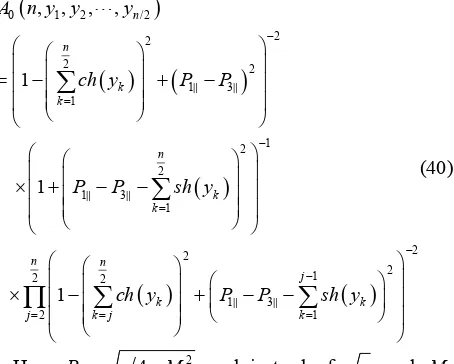
We first consider in more detail the case of even number of particles n in the diagram of Figure 2. The scattering amplitude reduction A n y y0( , , , ,1 2  yn/ 2) defined by

Equation (28) undimensioned by mass m takes a form:





 





 

 

 

0 1 2 / 2

2 2

2 ₂

1 3 1

1 2 2

1 3 1

2 2

2 1

2 2

1 3 1 2

, , , ,

1

1

1

n n

k k

n k k n n

j

k k

k j k

j

A n y y y

ch y P P

P P sh y

ch y P P sh y













 



 _{ } 

 _{ } 

 _{  }   _

 

 _{ } 

 

 _{ } 

 _{ } 

 _{ }   _{ }

 

 _{ } 

 

 _{ } 

     

 _ _{ } _   _{ }

 

 

 _{ } 

 











 

 

 



(40)

Here 2

1|| 4

P  s M and instead of s and M

we use their dimensionless by mass m values. Since we search for the constrained extremum, under condition of energy-momentum conservation, it is assumed that P3

is described by Equation (26), in which again all values are undimensioned by mass m. In particular, taking into account the symmetry relation, normalization and the introduction of rapidity (see Equation (15)), we obtain for Ep instead Equation (7):

 

2

1

2

n

p k

k

E s ch y



 



(41)

For further calculations we use the following denota- tion

 

2

1

n k k

E ch y







and  P P1P3 (42)

Note that due to Equations (26), (41) and (42) quantity

P

 depends on rapidity as the composite function of E, which is denoted as P E( ) and the first term of Equa-tion (40) depends on rapidity only via E.

Instead of looking for the maximum of function





0 , , , ,1 2 n/ 2

A n y y  y we can look for the maximum of its logarithm, which we define as L:

 









 

 

 

 

 

2 2

2

2 1

2 2

2 1

2 2

1

2 ln 1

2 ln 1

ln 1

n n

j

k k

j k j k

n k k

L E P E

ch y P E sh y

P E sh y



  



    

 _{ } 

 _{ }   

 _ _{ }  _  _{ }

 

 

 _{ } 

 

 _{ } 

 _{ } 

 _  _  _{ }

 

 _{ } 

 









 





 

 

 

 

 

2 2 1 2 2 1 2 1 2 2 1 ₁ 2 1 1 ,

1, 2, , 2

1

n

j

j k k

k j k

n

n k

k

Z E P E

Z ch y P E sh y

n j

Z P E sh y

    _            _{ }  _  _              _  _    







 (44)

Since after taking into account Equation (7), all vari-ables of function A n y y₀



, , , ,_{1 2}  y_{n/ 2}



and hence loga-rithm became independent, then the extreme point can be found under condition that partial derivatives with re-spect to all variables are equal to zero. The equations for the extreme point problem can be written down in a form:

 

 

 

 

 

 

 

1 2 1 1 1 2 1 2 1 1 1 2 4 2 0 j n k k j j n k k n

P E sh y

L L

sh y ch y

y E Z

P E sh y

ch y Z                 







(45)

 

 

 

 

 

 

 

2 2 1 2 1 1 2 1 1 2 4 4 ( )

2 ( ) 0

n k l k j l l j l j j n k k l

j l j

n k k l n ch y L L

sh y sh y

y E Z

P E sh y

ch y

Z

P E sh y

ch y Z                     











(46)

where 2, 3, , 1 2 n

l   .









 





 

 

/2

2 2

/ 2 / 2

2 2 1 / 2 1 2 4 2 0 n n n k k j n n j y j n k k n n ch y L L

sh y sh y

y E Z

P E sh y

ch y Z              







(47)

Equations (45)-(47) form the system of equations for

the extreme point search. An approximate solution of this system is the purpose of this section. The simplification of this system of equations can be attained in approximation, which we call “the equal-denominators approximation”.

As seen from Equation (36), the amplitude is a product of fractions whose denominators contain the expression greater than unit. However, function f x( ) 1 x slowly varying at x1, that follows from its derivative. In addition, as discussed in Section 3, virtualities increase, and hence, as it evident from Equation (38) and argu-ments made after this relation, the denominators increase with movement from the edges of the “comb” to its cen-ter. However, as we are looking for the maximum point, virtualities at this point should be as small as possible. Therefore, they should increase as we move from the edges of the “comb” to the center as slowly as possible. Hence, we can expect that the denominators lightly dif-fers from each other in the desired maximum point, then for the further analysis of the system of equations at the maximum point we adopt an approximation, in which all the denominators are equal between themselves. Their approximate common value will be denoted as Z,

, 1, 2, , 1

2

j

n

Z Z j   . (48) The equations for the maximum point as result of the approximation take form

 

 

 

 

 

 

 

 

1 2 1 2 1 1 2 1 1 1 2 2 0 n j k j k n k k ch y Z L

P E sh y

E sh y

ch y

P E sh y

sh y        _{  }    _{ }      _  _    







(49)

 

 

 

 

 

 

 

 

 

2 2 1 2 1 1 2 1 2 2 2 0 n l k j k j

n

j l

k

j l k

l n l k k l

Z L _{ch y}

E

ch y

P E sh y

sh y

ch y

P E sh y

sh y           _{ }  _{ }  _{ }      _  _        _  _    

 







(50)

here 2, 3, , 1 2 n

l  

 









 

 

2 2 2 2 / 2 1 / 2 2 2 0 n n k j k j

n n

k k n

Z L _{ch y}

E

ch y

P E sh y