A law of nature?

A law of nature?

Marvin Chester

Physics Department, University of California Los Angeles, Los Angeles, USA; chester@physics.ucla.edu

Received 20 September 2011; revised 21 October 2011; accepted 30 October 2011.

ABSTRACT

Is there an overriding principle of nature, hith-erto overlooked, that governs all population be- havior? A single principle that drives all the re- gimes observed in nature—exponential-like gr- owth, saturated growth, population decline, po- pulation extinction, oscillatory behavior? In cur- rent orthodox population theory, this diverse range of population behaviors is described by many different equations—each with its own sp- ecific justification. The signature of an overrid-ing principle would be a differential equation which, in a single statement, embraces all the panoply of regimes. A candidate such governing equation is proposed. The principle from which the equation is derived is this: The effect on the

environment of a population’s success is to alter that environment in a way that opposes the success.

Keywords: Population Dynamics; Ecology; Population Evolution; Exponential Growth; Eco-Evolutionary Dynamics; Biology

1. INTRODUCTION

What are the conceptual foundations in ecological stu- dies? Are there laws of nature governing ecological sys-tems? What are they?

Over the years there has grown a community of sch- olars who have grappled with these profound questions. [1-7] Some have concluded that concern for such laws is not the business of ecological research. [8,9] Others ha- ve concluded that Malthusian exponential growth con- stitutes an essential law [10]. That exponential growth and the logistics equation are of great conceptual utility but not laws of nature is argued cogently by still others [11,12].

Focussing on the lofty notion, Law of Nature, may be a distraction from a more elemental pursuit: to unders- tand nature. That is surely the goal of science. Progress in understanding is marked by conceptual coalescence:

the quest to embrace an ever larger body of findings with ever fewer statements of principle. Paraphrasing Mark Twain, the task of science is to describe a plethora of phenomena with a paucity of theory.

Newton showed that the motion of things on earth are governed by the same rules as the motions of heavenly bodies. Formerly these two had appeared to be unrelated domains. Newton showed that a single principle gover- ned them both. This synthesis was magnificently fruitful. It underlies our understanding of anything mechanical or structural. Much of our material well being depends on it.

Darwin’s principle of natural selection explained a wealth of biological phenomena by a single idea. Throu- gh his synthesis the concept of evolution became part of our intellectual heritage.

Wegener showed us that continental drift—plate tecto- nics—is the underlying reason for such diverse phenom- ena as the distribution of fossils in the world, the shape of continents, earthquake belts and volcanic activity. That insight has proved remarkably beneficial.

Mendeleev gave structure to the chaos of chemistry with his table of the elements. He consolidated a profu- sion of chemical data into an all encompassing tabular statement of principle. This undertaking led to the under- standing that matter was made of atoms. (Mendeleev, himself, never believed this!)

James Maxwell brought electricity and magnetism together by an overriding formalism that covered them both. The undertaking gave rise to an understanding of the nature of light.

the theory. Einstein’s laws of nature absorbed Newton’s. Relativity spawned nuclear energy, a deeper understand- ing of stellar processes and much more.

All of these examples have in common that a wide breadth of empirical observation is accounted for by a single idea. We see in them that conceptual coalescence is a foundation stone of scientific understanding. In that spirit, offered here is a candidate synthesis: a single equ- ation that brings together the disparate domains of popu- lation behavior. We suggest that the panoply of popula- tion behaviors all issue from a single principle.

In current orthodox population theory, the diverse ran- ge of population behaviors is described by many differ- ent equations—each with its own specific justification. Every regime has its own special theoretical rationale. Exponential growth has a limited range of validity. The Logistics Equation describes another restricted regime. Oscillatory behavior demands that a new paradigm be requisitioned; the Lotka-Volterra equations [13,14] or, because their solutions are not structurally stable, their later modifications [15,16]. And none of these describe population decline, nor population extinction. Contem- porary theory offers no overriding principle that governs the entire gamut of population behaviors.

As long ago as 1972 [17], in a challenge to orthodox convention, L. R. Ginzburg took the bold step of pro-posing that population dynamics is better represented by a second order differential equation. All accepted for-mulations relied on first order differential equations as they still do today. He developed his thesis over the years [18-21] culminating in the pithy and persuasive book, “Ecological Orbits” [4].

When the family of solutions to a differential equation is found to fit empirical reality then that equation is ex- pressing a truth about nature. It can give us insights and enable us to make predictions. Producing a second order equation whose solutions characterize a variety of popu- lation behavior is equivalent to uncovering a principle of nature governing those populations.

In the following we take a route different from Gin- zburg’s and arrive at a substantially different equation - albeit a second order one. We procede from a guess at what may be the underlying principle and then derive the second order differential equation that expresses that principle. If empirical reality is well fit by the progeny of that equation then we may conclude that the principle is true. And we will have produced a conceptual coales- cence: a tool for better understanding nature.

2. TRADITIONAL PERSPECTIVE

Call the number of members in the population, n. At each moment of time, t, there exist n individuals in the population. So we expect that n = n(t) is a continuous

function of time.

The rate of growth of the population is dn/dt; the in-crease in the number of members per unit time. That this is proportional to population number, n, is the substance of Malthus’ idea of “increase by geometrical ratio”. Call the constant of proportionality, R. Then the well known differential equation that embodies the idea is:

dn dt =Rn (1) It is a first order differential equation and when R is constant, its solution yields the archetypical equation of exponential growth.

Now, common experience tells us that exponential gr- owth cannot proceed indefinitely. “Most populations do not, in fact, show exponential growth, and even when they do it is for short periods of time in restricted spatial domains,” writes R.D. Holt [12]. No population grows without end.

The first efforts to expand the breadth of applicability of theory to observation—to acheive some conceptual coalescence—was to allow R to vary with time. The motivation was to retain that appealing exponential-like form and seek to explain events by variations in R. “The problem of explaining and predicting the dynamics of any particular population boils down to defining how R deviates from the expectation of uniform growth” [10]. The concept is that exponential growth is always taking place but at a rate that varies with time. The idea is ubiquitous in textbooks [15,22-24].

An object example of this process is provided by the celebrated Verhulst equation.

 

dn n

=nR n =nr 1 dt   K



 (2)

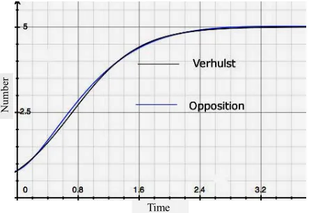
Here the constant, r, is the exponential growth factor and K is the limiting value that n can have - “the carry-ing capacity of the environment” [16]. The equation in-sures that n never gets larger than nMAX = K. A popula-tion history, n vs. t, resulting from this first order differ-ential equation is the black one of Figure 1. The Ver-hulst equation—often cited as the Logistics Equation—is regularly embedded in research studies [25-30].

3. SHORTCOMINGS OF THE

TRADITIONAL PERSPECTIVE

bed in this formalism.

Another proscribed regime is extinction. A phenome- non well known to exist in nature is the extinction of a species. “... over 99% of all species that ever existed are extinct” [31]. But there exists no finite value of R—posi- tive or negative—that yields extinction! It cannot be rep- resented by R except for the value negative infinity; –∞. So, in fact, there is good reason to avoid R as the key parameter of population dynamics.

In the continuous n perspective the mathematical con- ditions for extinction are these: n = 0 and dn/dt < 0. No infinities enter computations founded on these statements. Hence embracing n(t) itself as the key variable directly allows one to explore the dynamics of extinction.

Next consider the eponymous Verhulst Eq.2, the Lo-gistics Equation. As Verhulst himself pointed out [32] it is motivated only by the observation that populations never grow to infinity. They are bounded.

But there are other ways—not describable by Verhul- st’s equation—in which population may be bounded. For example, n(t) may exhibit periodicity. Or, as in Figure 1, a curve essentially the same as Verhulst’s may arise from an entirely different theory where no K = nmax limit ex-ists. One of the possible population histories resulting from the alternative theory offered below—which con-tains no nmax—is shown in blue. Data fit by one curve will be fit just as well by the other. The limited validity of r/K Selection Theory has been noted by researchers over the years[33,34].

Thus the accepted Malthusian Structure of population dynamics has, and will always have, only a limited do- main of validity. Many population histories cannot be fit with this structure no matter how R is allowed to vary.

So, in current orthodox population theory, to describe the entire range of population behaviors requires many

Figure 1. Two population histories: number vs. time. The black

curve is the Verhulst (Logistics) Equation. The blue curve is one of the solutions to the Opposition Principle differential Equation (8). Where one curve fits data so will the other.

different equations—each with its own specific justifica-tion. Exponential growth has a limited range of validity, as does the Logistics Equation, and any other equation of first order. Oscillatory behavior demands that a new pa- radigm be requisitioned; the Lotka-Volterra equations. And none of these describe population decline, nor ex-tinction.

No structure exists that embraces—in one single sta- tement—all possible behaviors. Contemporary theory of- fers no overriding principle that governs the gamut of population behaviors. To produce such a structure is the aim of what follows.

4. CONCEPTUAL FOUNDATIONS FOR

AN OVERRIDING STRUCTURE

We seek a mathematical structure to embrace all of the great variety of population behaviors. The equation is built on some foundational axioms. Empirical verifica- tion of the equation they produce is what will measure the validity of these axioms. The axioms are:

First: Variations in population number, n, are due en-tirely to environment.

Conceptionally we partition the universe into two: the population under consideration and its environment. We assume that the environment drives population dynamics; that the environment is entirely responsible for time variations in population number—whether within a sin- gle lifetime or over many generations.

The survival and reproductive success of any individ- ual is influenced by heredity as well as the environment it encounters. This statement doesn’t contradict the axi- om. The individual comes provisioned with heredity to face the environment. Both the environment and the po- pulation come to the present moment equipped with their capacities to influence each other; capacities derived fr- om their past histories.

That the environment molds the population within a li- fetime is clear; think of a tornado, a disease outbreak, or a meteor impact. That the environment governs population dynamics over generations is precisely the substance of “natural selection” in Darwinian evolution.

Nu

m

be

r

That principle may be summarized as follows: “... the small selective advantage a trait confers on individuals that have it...” [31] increases the population of those individuals. But what does ‘selective advantage’ mean? It means that the favored population is ‘selected’ by the environment to thrive. Ultimately it is the environment that governs a population’s history. Findings in epigene- tics that the environment can produce changes transmit-ted across generations [35,36] adds further support to this notion.

Time

ductive Success) [37,38]. The focus is on how the orga- nism fits into its environment. So something called “fit- ness” is attributed to the organism; the property of an organism that favors survival success. But environmen- tal selection from among the available phenotypes is what determines evolutionary success. The environment is always changing so whatever genetic attributes were favorable earlier may become unfavorable later. Hence there is an alternative perspective: fitness, being a matter of selection by the environment, is induced by it and may, thus, be seen as a property of the environment.

Although, fitness, in some sense, is “carried” by the genome, it is “decided” by the environment. Assigning a fitness to an organism rests on the supposition of a static environment; one into which an organism fits or does not fit. A dynamic environment incessantly alters the “fitness” of an organism.

This is the perspective underlying the axiom that va- riations in population number, n, are due entirely to en-vironment.

In this view, although birth rates minus death rates yield population growth they are not the cause of popu- lation dynamics; rather birth and death rates register the effect of the environment on the population. This view parallels that of N. Owen-Smith who writes: [39] “... population growth is not the result of a difference be- tween births and deaths (despite the appearance of this statement in most text-books), but rather of the differ-ence between rates of uptake and conversion of reso- urces into biomass, and losses of biomass to metabolism and mortality.”

Second: An increasing growth rate is what measures a population’s success.

The “success” of a population is an assertion about a population’s time development; it concerns the size and growth of the population. A reasonable notion of success is that the population is flourishing. We want to give quantitative voice to the notion that flourishing growth reveals a population’s success.

Neither population number, n, nor population growth, dn/dt, are adequate to represent “flourishing”. Population number may be large but it may be falling. Such a popu-lation cannot be said to be flourishing. So we can’t use population number as the measure of success. Growth seems a better candidate. But, again, suppose growth is large but falling. Only a rising growth rate would indi- cate “flourishing”. This is exactly the quantity we propo- se to take as a measure of success; the growth in the gr- owth rate. By flourishing is meant growing faster each year. That the rate of change of growth is a fundamental consideration in population dynamics has been advoca- ted in the past [4].

A corollary of these two foundational hypotheses is that change is perpetual. Equilibrium is a temporary

condition. What we call equilibrium is a stretch of time during which dn/dt = 0. Hence “returning to equilibrium” is not a feature of analysis in this model. “Biological persistence (is) more a matter of coping with variability than balancing around some equilibrium state.” [40]

Another corollary is this: The environment of one population is other populations. It’s through this mecha- nism that interactions among populations occur: via reci- procity—if A is in the environment of B, then B is in the environment of A. So the structure offers a natural set- ting for “feedback” [41]. It provides a framework for the analysis of competition, of co-evolution and of preda- tor-prey relations among populations. These obey the sa- me equation but differ only in the signs of coefficients relating any pair of populations.

5. THE OPPOSITION PRINCIPLE:

QUANTITATIVE FORMULATION

Based on the understandings outlined above we pro- pose that an overriding principle governs the population dynamics of living things. It is this: The effect on the environment of a population’s success is to alter that environment in a way that opposes the success. In order to refer to it, I call it the Opposition Principle. It is a functional principle [42] operating irrespective of the mechanisms by which it is accomplished. In the way that increasing entropy governs processes irrespective of the way in which that is accomplished.

The Principle applies to a society of living organisms that share an environment. The key feature of that soci-ety is that it consists of a number, n, of members which have an inherent drive to survive and to produce off-spring with genetic variation. Their number varies with time: n = n(t).

Because we don’t know whether n, itself, or some monotonically increasing function of n is the relevant parameter, we define a population strength, N(n). Any population exhibits a certain strength in influencing its environment. This population strength, N(n), expresses the potency of the population in affecting the environ-ment—its environmental impact.

N. Owen-Smith [39] urges us to “assess abundance” in terms of biomass rather than population. What is here named “population strength” is related to that idea. Population number, itself, may not be a measure of en-vironmental potency.

Two things about the population potency, N, are clear. First, N(n) must be a monotonically increasing function of n; dN/dn > 0. This is because when the population increases then its impact also increases. Albeit, perhaps not linearly. Second, when n = 0 so, too, is N = 0. If the population is zero then certainly its impact is zero. One candidate for N(n) might be n raised to some positive power, p. If p = 1 then N and n are the same thing. An-other candidate is the logarithm of (n + 1).

We need not specify the precise relationship, N(n), in what follows. Via experiment it can be coaxed from na-ture. The only way that N depends upon time is para-metrically through its dependence on n. In what follows we shall mean by N(t) the dependence N(n(t)). We may think of N as a surrogate for the number of members in the population.

The population strength growth rate, g = g(t), is de-fined by

dN g:=

dt (3) Like N, g too acquires its time dependence paramet- riccally through n(t). g = (dN/dn)(dn/dt).

To quantify how the environment affects the popula- tion we introduce the notion of “environmental favorabi- lity”. We’ll designate it by the symbol, f. It represents the effect of the environment on the population.

A population flourishes when the environment is favo- rable. Environmental favorability is what drives a popu- lation’s success. We may be sure that food abundance is an element of environmental favorability so f increases monotonically with nutrient amount. It decreases with predator presence and f decreases with any malignancy in the environment—pollution, toxicity.

But in the last section we arrived at a quantitative measure of success. The rate of growth of the population strength—“the growth of growth” or dg/dt—measures success. Hence, that a population’s success is generated entirely by the environment can be expressed mathema- tically as:

dg =f

dt (4) By omitting any proportionality constant we are de-claring that f may be measured in units of (time)–2_{. Since}

Eq.4 says that success equals the favorability of the en-vironment, it follows that f measures not only environ-mental favorability but also population success. One can gauge the favorability of the environment—the value of f—by measuring population success.

We’re now prepared to caste the Opposition Principle as a mathematical statement. The Principle has two parts: 1) Any increase in population strength decreases favora- bility; the more the population’s presence is felt the less

favorable becomes the environment. 2) Any increase in the growth of that strength also decreases favorability.

Put formally: That part of the change in f due to an increase in N is negative. Likewise the change in f due to an increase in g is negative. Here is the direct mathema- tical rendering of these two statements:

f

0 and 0

N g

f

 _  _

  (5)

We can implement these statements by introducing two parameters. Both w and  are non-negative real numbers and they have the dimensions of reciprocal time. (Negative w values are permitted but are redundant.)

2

f f

and

N w g 

 

 

   

t

(6)

These partial differential equations can be integrated. The result is:

 

2

f  w Ng F (7) The “constant” (with respect to N and g) of integra-tion, F(t), has an evident interpretation. It is the gratui-tous favorability provided by nature; the gift of nature. Eq.7 says that environmental favorability consists of two parts.

One part depends on the number and growth of the population being favored: the N and its time derivative, g. This part has two terms both of which always act to decrease favorability. These terms express the Opposi- tion Principle.

The other part—F(t)—is the gift of nature. There must be something in the environment that is favorable to population success but external to that population else the population would not exist in the first place. This gift of nature may depend cyclically on time. For example, seasonal variations are cyclical changes in favorability. Or it may remain relatively constant like the presence of air to breathe. It may also exhibit random and sometimes violent fluctuations like a volcanic eruption or unex- pected rains on a parched earth. So it has a stochastic component. All of these are independent of the popula-tion under considerapopula-tion. In fact, however, dF/dt may depend on population number since this is the rate of consumption of a limited food supply.

Inserting Eq.3,4,7 we arrive at the promised differen-tial equation governing population dymics under the Opposition Principle. It is this.

 

2

2 2

d N dN

+ + N=

dt

other phenomena. So it is very well studied. The exact analytical solution to (8), yielding N(t) for any given F(t), is known.

6. FITS TO EMPIRICAL DATA

To explore some of the consequences of this differen-tial equation we consider the easiest case; that the gift favorability is simply constant over an extended period of time. Assume F(t) = c independent of time. Non-peri- odic solutions arise if ≥ 2w. As displayed in Figure 1 these produce results similar to the Verhulst equation— the Logistics equation. And like that equation they exhi- bit an exponential-like growth over a limited range.

Empirical data on such an exponential-like growth is exhibited in Figure 2 showing the population of musk ox (Ovibos moschatus) isolated on Nunivak Island in Al- aska [43]. The data, gathered every year from 1947 to 1968, is in Table 1 of Spencer and Lensink’s paper. It is, indeed, well fit by an exponential curve showing the formidable growth rate of 13.5% per year.

The population cannot possibly fit such a curve in-definitely. Nothing grows without end. The exponential curve fits the population data only in the domain shown. But, in this domain, the data is also well fit by an Oppo-sition Principle curve where = 0.02 per year, w = 0.0076 per year and n = N.

If < 2w the solutions to (8) are periodic and are given by:

 





2

N t c Ae t sin t w

 _



  a

Principle curve may be fit to the data.

gnated time, say

(9)

where the amplitude, A, and the phase, a, depend upon

Figure 2. Data points, gathered every year from 1947 to 1968,

reporting the number of musk ox on Nunivak Island, Alaska. The curves show that both an exponential and an Opposition

the conditions of the population at a desi

t = 0. And the oscillation frequency, is given by:

2

 

: 1

2 w

w

   _ _ _ _

 

  (10)

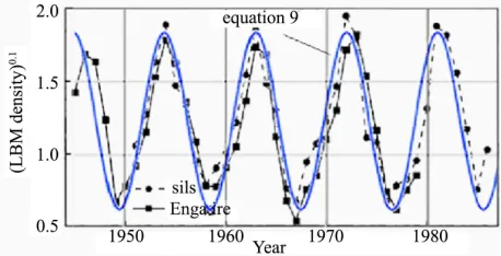
In Figure 3, Eq.9 is compared to empirical data. The fig

set eq

fluctuations are so large the authors plot-te

ed are these: s of bu

ces in which popu- lation ex

ure shows the population fluctuations of larch bud-moth density [44] assembled from records gathered over a period of 40 yr. The data points and lines connecting them are shown in black. The smooth blue curve is a graph of Eq.9 for particular values of the parameters.

We assumed is negligibly small so it can be ual to zero. The frequency, is taken to be 2/(9 yr) = 0.7 per year. The vertical axis represents N. In the units chosen for N, the amplitude, A, is taken to be 0.6 and c is taken to be 0.6 per year2_{. The phase, a, is chosen so as} to insure a peak in the population in the year 1963; a = 3.49 radians.

Because the

d n0.1 _{as the ordinate for their data presentation. The} ordinate for the smooth blue theoretical curve is N. Looking at the fit in Figure 3, suggests how population potency may be deduced from empirical data. One is led to conclude that the population strength, N(n), for the budmoth varies as the 0.1 power of n. But the precision of fit may not warrant this conclusion.

The conclusions that may be warrant

Considering that no information about the detail dmoth life have gone into the computation the gra- phical correspondence is noteworthy. It suggests that those details of budmoth life are nature’s way of imple- menting an overriding principle. The graphical corres- pondence means that, under a constant external environ- mental favorability, a population should behave not un- like that of the budmoth.

Eq.9 admits of circumstan

tinction can occur. If A > c/w2 then N can drop to zero. Societies with zero population are extinct ones. (On at-

P

opul

at

io

n

Year

Figure 3. Observational data on the population fluctuations of

ing differential

initial conditions; fr- om

se explored reveals that periodic population os-ci

he plethora of solutions to the governing dif- fe

monds) of Figure 5 record the po

taining zero, N remains zero. The govern Eq.8, doesn’t apply when N < 0.)

But the value of A derives from

N(t = 0) and g(t = 0). So depending upon the seed population and its initial growth rate the population may thrive or become extinct even in the presence of gift fa- vorability, c. This result offers an explanation for the ex- istence of the phenomenon of “extinction debt” [45] and a way to compute the relaxation time for delayed exti- ncttion.

The ca

llations can occur without a periodic driving force. Ev- en a steady favorability can produce population oscilla-tions.

Among t

rential Eq.8, is this one: Upon a step increase in envi-ronmental favorability—say, in nutrient abundance—the population may overshoot what the new environment can accommodate and then settle down after a few cy-cles. Figure 4 illustrates this behavior. That there are such solutions amounts to a prediction that population histories like that of Figure 4 will be found in nature. In fact it has been found.

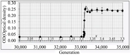
The data points (dia

pulation of Escherichia coli (using optical density, OD, to measure it) maintained over 30,000 generations on a nutrient containing citrate which it could not exploit [46]. Around generation 33,100 a mutation arose allowing a

Figure 4. A theoretical population history that can result f om

Figure 5. Fit of Opposition Principle curve to the data on a

str-occurs in the favorability of its environment.

CLUSIONS

sparate regimes of population

REFERENCES

(2000) Universal laws and predictive nd evolution. Oikos, 89, 403-408.

r the Opposition Principle differential equation.

ain of E coli for which, because of a mutation, a step increase

strain of the species to exploit this nutrient component. For those with this mutation the environment became suddenly more favorable and they flourished. Shown in the same figure is the theoretical curve arising from the Opposition Principle Eq.8 with parameters = 0.028 per generation and w = 0.023 per generation and n = N1.32_.

7. CON

We noted at least five di

history—each with it’s own individual and disjoint desc- riptive equation: exponential-like growth, saturated growth, population decline, population extinction, and oscillatory behavior. Another regime, without a theory, is population overshoot. It’s argued here that these regimes can be brought under the embrace of a single differential equa-tion describing them all.

That equation is the mathematical expression of gen-eral concepts about how nature governs population be-havior. Being quantitative it offers us a framework with which to validate or refute these concepts. They are itemized as axioms and principles (Section 4). Some of these run counter to accepted convention thus making empirical refutation a substantive matter. In short: a re-futable proposition about the nature of populations is offered for assessment by the scientific community. Verification of the proposed equation would establish a basic understanding about the nature of living organ-isms.

[1] Murray, B.G., Jr. theory in ecology a

doi:10.1034/j.1600-0706.2000.890223.x

[2] Murray Jr., B.G. (2001) Are ecological and evolution theories scientific? Biological Reviews, 76

ary , 255-289.

doi:10.1017/S146479310100567X

[3] Turchin, P. (2001) Does population ecology have gene laws? Oikos, 94, 17-26.

ral

doi:10.1034/j.1600-0706.2001.11310.x

[4] Ginzburg, L.R. and Coly

Oxford University Press, Oxford. van, M. (2004) Ecological orbits.

, 110, 394-403.

[5] Lange, M. (2005) Ecological laws: What would they be and why would they matter? Oikos

O

D

(O

ptic

al

d

ens

it

y)

Generation

doi:10.1111/j.0030-1299.2005.14110.x

[6] Gorelick, R. (2011) What is theory? Ideas in Ecology Evolution, 4, 1-10.

and

oking beyond disciplinary boundaries. [7] Colyvan, M. and Ginzburg, L.R. (2010) Analogical thin-

king in ecology: Lo

The Quarterly Review of Biology, 85, 1-12. doi:10.1086/652321

[8] Egler, F.E. (1986) Physics envy in ecology. the Ecology Society o

Bulletin of f America, 67, 233-235.

, 110,

ology. Oikos, 103, 695-701.

390-393.

[10] Berryman, A. (2003) On principles, laws and theory in po- pulation ec

doi:10.1034/j.1600-0706.2003.12810.x

[11] Lockwood, D.R. (2008) When logic fail terly Review of Biology, 83, 57-64.

s ecology. Qua-0.1086/529563 doi:1

[12] Holt, R.D., (2009) Darwin, malthus and movement: A hidden assumption in the demographic foundations of evolution. Israel Journal of Ecology and Evolution, 55,

189-198. doi:10.1560/IJEE.55.3.189

[13] Lotka, A.J. (1956) Elements of mathematical biology. Dover, New York.

[14] Volterra, V. (1926) Fluctuations in the abundance of a species considered mathematically. Nature, 118, 558-560 doi:10.1038/118558a0

[15] Murray, J.D. (1989) Mathematical biology. Springer-Ver- lag, Berlin.

[16] Vainstein, J.H., Rube, J.M. and Vilar, J.M.G. (2007) Sto- chastic population dynamics in turbulent fields. Euro- pean Physical Journal Special Topics, 146, 177-187. doi:10.1140/epjst/e2007-00178-7

[17] Ginzburg, L.R. (1972) The analogies of the “free motio and “force” concepts in population theory (in Russian). n”

l Bi- In: Ratner, V.A. Ed., Studies on theoretical genetics, Aca- demy of Sciences of the USSR, Novosibirsk, 65-85. [18] Ginzburg, L.R. (1986) The theory of population dynamo-

ics: I. Back to first principles. Journal of Theoretica ology122, 385-399. doi:10.1016/S0022-5193(86)80180-1

[19] Ginzburg, L.R. (1992) Evolutionary consequences of ba- sic growth equations. Trends in Ecology and Evolution, 7,

133. doi:10.1016/0169-5347(92)90149-6

[20] Ginzburg, L.R. and Taneyhill, D. (1995) Higher growth rate implies shorter cycle, whatever the cause: A reply to Berryman. Journal of Animal Ecology, 64, 294-295. doi:10.2307/5764

[21] Ginzburg, L.R. and Inchausti, P. (1997) Asymmetry of p pulation cycles: Ab

o- undance-growth representation of hid- den causes of ecological dynamics. Oikos, 80, 435-447. doi:10.2307/3546616

[22] Britton, N.F., (2003) Essential mathematical biology. Sprin- ger, London.

[23] Turchin, P. (2003) Complex population dynamics: A theo- retical/empirical synthesis. Princeton University Press, Prin-

iley and Sons, New York.

s,Cambridge.

nviron- ceton.

[24] Vandemeer, J., (1981) Elementary mathematical ecology. John W

[25] Nowak, M.A. (2006) Evolutionary dynamics: Exploring the equations of life. Harvard Pres

[26] Torres, J.-L., Pérez-Maqueo, O., Equihua, M. and Torres, L. (2009) Quantitative assessment of organism-e ment couplings. Biology and Philosophy, 24, 107-117. doi:10.1007/s10539-008-9119-9

[27] Jones, J.M. (1976) The r-K-Selection Continuum. The Am rican Naturalist, 110, 320-323.

e- i:10.1086/283069 do

[28] Ruokolainen, L., Lindéna, A., Kaitalaa, V. and Fowler, M.S. (2009) Ecological and evolutionary dynamics under coloured environmental variation. Trends in Ecology and Evolution, 24, 555-563. doi:10.1016/j.tree.2009.04.009

[29] Okada, H., Harada, H., Tsukiboshi, T. and Araki, M. (2005) Characteristics of Tylencholaimus parvus (Nema-toda: Dorylaimida) as a fungivorus nematode. Nematol-ogy, 7, 843-849. doi:10.1163/156854105776186424

[30] Ma, Z.S. (2010). Did we miss some evidence of chaos in laboratory insect populations? Population Ecology, 53,

405-412. doi:10.1007/s10144-010-0232-7

[31] Carroll, S.B. (2006) The Making of the fittest. W.W. Nor- ton, New York.

[32] Verhulst, P.-F., (1838) Notice sur la loi que la population poursuit dans son accroissement. Correspondance Mathé-

7/BF00347974 matique et Physique, 10, 113-121.

[33] Parry, G.D. (1981) The meanings of r- and K-selection. Oecologia, 48, 260-264. doi:10.100

r arti-[34] Kuno, E. (1991) Some strange properties of the logistic

equation defined with r and K—inherent defects o facts. Researches on Population Ecology, 33, 33-39. doi:10.1007/BF02514572

[35] Gilbert, S.F. and Epel, D. (2009) Ecological developme tal biology. Sinauer, Sunde

n- rland.

isms and implica- [36] Jablonka, E. and Raz, G. (2009) Transgenerational epige-

netic inheritance: Prevalence, mechan

tions for the study of heredity and evolution. Quarterly Review of Biology, 84, 131-176. doi:10.1086/598822

[37] Clutton-Brock, T.H. (Ed.) (1990) Reproductive success: Studies of individual variation in contrasting breeding

ating in- systems. University of Chicago Press, Chicago.

[38] Coulson, T., Benton, T.G., Lundberg, P., Dall, S.R.X., Kendall, B.E. and Gaillard, J.-M. (2006) Estim

dividual contributions to population growth: Evolution- ary fitness in ecological time. Proceedings of the Royal Society B, 273, 547-555. doi:10.1098/rspb.2005.3357

[39] Owen-Smith, N. (2005) Incorporating fundamental laws of biology and physics into population ecology: The me- taphysiological approach. Oikos, 111, 611-615.

doi:10.1111/j.1600-0706.2005.14603.x

[40] Owen-Smith, R.N. (2002) Adaptive herbivore

Cambridge University Press, Cambridge. ecology.

doi:10.1017/CBO9780511525605

[41] Pelletier, F., Garant, D. and Hendry, A.P. (20 lutionary dynamics. Phililosophica

09) Eco-evo- l Transactions Royal Society B, 364, 1483-1489. doi:10.1098/rstb.2009.0027

[42] McNamara, J.M. and Houston, A.I. (2009) Integrating fun- ction and mechanism. Trends in Ecology and Evolution, 24, 670-675. doi:10.1016/j.tree.2009.05.011

[43] Spencer, C.L. and Lensink, C.J. (1970) The muskox of Nu- nivak Island, Alaska. The Journal of Wildlife Manage-ment, 34, 1-15. doi:10.2307/3799485

[44] Turchin, P., Wood, S.N., Ellner, S.P., Kendall, B.E., Mur- doch, W.W., Fischlin, A., Casas, J., McCauley, E. and Bri- ggs, C.J. (2003) Dynamical effects of plant quality and parasitism on population cycles of larch budmoth. Ecol- ogy, 84, 1207-1214.

doi:10.1890/0012-9658(2003)084%5B1207:DEOPQA% 5D2.0.CO;2

[45] Kuussaari, M., Bommarco, R., Heikkinen, R.K., Helm, A., Krauss, J., Lindborg, R., Öckinger, E., Pärtel, M., Pi- no, J., Rodà, F., Stefanescu, C., Teder, T., Zobel, M. and Ingolf, S.-D.I. (2009) Extinction debt: A challenge for biodiversity conservation. Trends in Ecology and Evolu-tion, 24, 564-571. doi:10.1016/j.tree.2009.04.011

[46] Blount, Z.D., Boreland, C.Z. and Lenski, R.E. (2008) His- torical contingency and the evolution of a key innovation in an experimental population of Escherichia coli. Pro-ceedings of the National Academy of Science, 105, 7899-

7906. doi:10.1073/pnas.0803151105