System Identification of Wood Drying Process Based on ARMAX Model

ISSN Online: 2156-8561 ISSN Print: 2156-8553

DOI: 10.4236/as.2019.103020 Mar. 11, 2019 241 Agricultural Sciences

System Identification of Wood Drying Process

Based on ARMAX Model

Zheng Zhou, Pinxiu Zhang

, Baofu Huai, Liping Huang

Electrical and Information College, Heilongjiang Bayi Agricultural University, Daqing, China

Abstract

This article presents system identification of wood drying process based on ARMAX model. Temperature and equivalent moisture content are consid-ered as inputs, and moisture content of the wood sample during drying is taken as output of the system. The comparative study of RLS and FF-RLS to identify the system parameters is presented. Simulation results are presented to validate the efficacy of the ARMAX model for wood drying process.

Keywords

Wood Drying, System Identification, Moisture Content

1. Introduction

Wood drying process plays an important role in industry of wood product [1]. The quality of wood product mainly depends on the final moisture content of wood. Temperature and equilibrium moisture content (EMC) are the two main factors influencing the drying moisture content [2]. Hence, experimental data of temperature and EMC was often used to build the prediction model of wood drying moisture in the previous literature.

Wood drying prediction models like [3] [4] [5] [6], simplified physical cha-racteristics are used to simulate the coupled heat and mass transfer during wood drying. However, too many inputs, e.g., gravity, external pressure, capillarity, temperature gradient, water concentration, etc., used to build theoretical models has a deterioration in accuracy to solve the highly coupled equations. Mathe-matical method such as artificial neural networks (ANN) and support vector machines (SVM) have been used to build drying model due to their ability to capture the trend of moisture content [7] [8] [9] [10]. ANN model can provide accurate prediction results, however over-training problem must to be taken

How to cite this paper: Zhou, Z., Zhang, P.X., Huai, B.F. and Huang, L.P. (2019) System Identification of Wood Drying Process Based on ARMAX Model. Agri-cultural Sciences, 10, 241-248.

https://doi.org/10.4236/as.2019.103020

DOI:10.4236/as.2019.103020 242 Agricultural Sciences

care of to develop the prediction model. SVM model depends on a subset of training data points. Though incomplete data can be used to develop a SVM model, it also requires a substantial number of computation times to solve large-size equations [11].

Prediction models based on Auto Regressive Moving Average model with ex-ogenous input (ARMAX) analysis have been widely shown in literature [12] [13] [14] [15] because of the computational efficiency. To the best of authors’ know-ledge, ARMAX model applied in the field of wood drying have rarely been seen in the previous research. In this paper, the method of ARMAX is presented to describe the time-varying system of wood drying. Recursive Least Squares (RLS) is introduced to identify the coefficients of the ARMAX model. To improve the identifying accuracy, an optimization algorithm is also discussed. Wood sample used in this study for the drying experiment was Northeast China ash. The dying kiln and its inside structure are show in Figure 1. The temperature, EMC, and moisture content used in the simulation model were the average value collected by temperature sensors, EMC sensors, and moisture content sensors.

2. Mathematics Model Description

The model takes temperature and EMC as inputs, moisture content as output. ARMAX model of wood drying process is described as

1 1 2 2

( ) ( ) ( ) ( ) ( ) ( ) ( ) ( )

A z y t =B z u t +B z u t +D z v t ₍₁₎

The constant coefficient polynomials A z( ), B z1( ), B z2( ) in the wood

dry-ing process model are

1 2

0 1 2

( )

A z ₌a a z₊ − ₊a z− ₍₂₎

1 2

1( ) 10 1 2

B z ₌b ₊b z− ₊b z− ₍₃₎

1 2

2( ) 20 3 4

B z ₌b ₊b z− ₊b z− ₍₄₎

1

0 1

( )

D z ₌d ₊d z− ₍₅₎

When t≤0 , y t( ) 0= , u tj( ) 0= , v t( ) 0= , a0=1, b10 =0 , b20=0 ,

0 0

d = _.

Substituting polynomials (2), (3), (4), (5) and the initial values into (1), gives

1 2

1 2

1 2 1 2

1 2 1 3 4 2 1 1

1 (

( ) ( )

)

) )

( (

a z a z y t

b z b z u t b z b z u t d z vt

− − − − − − −         + +

=_ + _ +_ + _ + (6)

DOI:10.4236/as.2019.103020 243 Agricultural Sciences

Introducing the unit backward shift operator z−1 _{into (6) yields to}

(

)

(

)

(

)

(

)

(

)

(

)

1 2 1 1 2 1

2 4 2

3 1

( ) 1 2 1 2

1 2 ( 1)

y t a y t a y t b u t b u

d v t

t

b u t b u t

= − − − − + − + −

+ − + − + − (7)

Therefore, the output y t( ) can be expressed as

( ) ( ) ( )

y t ₌ϕΤ tθ₊v t ₍₈₎

where T

1 2 1 2 3 4 1

: [ , , , , , , ]a a b b b b d

θ = _, ϕ( )t _{= [−y(t − 1), −y(t − 2), u1(t − 1), u1(t −}

2), u2(t − 1), u2(t − 2),v(t − 1)]T.

3. Parameter Identification

Let t = 1, 2, ∙∙∙, Equation (8) leads to

t t t

Y =Hθ+V ₍₉₎

Using the Least Squares identification principle to define the quadratic crite-rion function

T T

( ) : t t ( t t ) ( t t )

J θ =V V = Y H− θ Y H− θ ₍₁₀₎

Using recursive method, matrix _{P t}−1_{( ) is define as}

1 1 T 1 T

0 1

( ) (0) t ( ) ( ) (0) t t, (0) 0

j

P t− P− ϕ ϕj j P− H H P p I

=

= +

∑

The RLS estimation of the parameter vector is

T 1 T T T T

ˆ_{( ) (t H Ht t) H Y P t H Yt t ( ) t t} ˆ_{( 1)t P t( ) ( )[ ( )t y t ( ) ( 1)]t t}ˆ θ ₌ − _{= =}θ _{− +} ϕ ₋ϕ θ _{− (12)}

The estimated residual is

ˆ ˆ

ˆ( ) ( ) ( ) ( )

v t = y t −ϕ θt t ₍₁₃₎

where ϕˆ( ) : [ ( ) , ( 1)]t ₌ φ t v tΤ ˆ ₋ Τ_.

RLS estimation of parameter vector θ _{is achieved} T

ˆ_{( )= ( 1)t} ˆ _{t P t( ) ( )[ ( )ˆ t y t ˆ ( ) ( 1)]t t}ˆ

θ θ − + ϕ −ϕ θ − ₍₁₄₎

1 1 T

0 ˆ ˆ

( ) ( 1) ( ) ( ), (0) 0

P t− ₌P t− _{− +}ϕ ϕt t P ₌ p I _{> (15)}

In experimental system, data accumulates with time, results in the failure of extracting new data information from the previous data. Especially to the time-varying parameter system, due to the characteristics of parameter, the algo-rithm should track the time variation parameter. Hence, forgetting factor λ is introduced into (15), an optimization algorithm to identify the parameters is obtained

1_{( )} 1_{( 1) ˆ( ) ( )ˆ}T

P t− ₌λP t− _{− +}ϕ ϕt t ₍₁₆₎

4. Simulation Results

4.1. Computation of the Model Parameters Based on RLS

DOI:10.4236/as.2019.103020 244 Agricultural Sciences

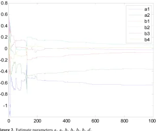
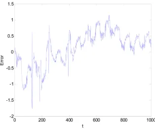
to estimate the parameters in the ARMAX model built in Equation (1). Parame-ters variation trend is shown in Figure 2. Comparison of actual values and dicted values are shown in Figure 3. Figure 4 is the absolute error between pre-dicted value and actual value. Mean Square Error (MSE) and Root Mean Square Error (RMSE) of RLS algorithm is 0.2973 and 0.5387, respectively.

Figure 2. Estimate parameters a1, a2, b1, b2, b3, b4, d1.

DOI:10.4236/as.2019.103020 245 Agricultural Sciences Figure 4. Absolute error.

4.2. Computation of the Model Parameters Based on FF-RLS

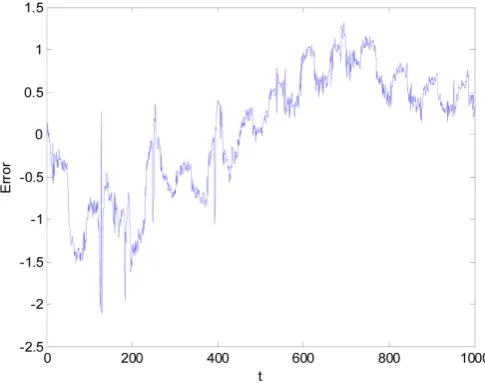
Parameters variation trend with λ = 0.95 is shown in Figure 5. It is obviously observed that the FF-RLS (Forgetting Factor Recursive Least Squares) algorithm has a faster convergence speed than RLS algorithm. From t = 200, curves of es-timate parameters tend to be stable. The comparison of actual values and pre-dicted values is shown in Figure 6. The absolute error between prepre-dicted value and actual values is shown in Figure 7. MSE is 0.3630, and RMSE is 0.7111. Convergence speed of FF-RLS algorithm is faster, however the absolute error is greater than RLS algorithm.

DOI:10.4236/as.2019.103020 246 Agricultural Sciences Figure 6. Comparison of actual values and predicted values.

Figure 7. Absolute error.

5. Conclusion

In this paper, an ARMAX model based on the experimental data is derived to describe the wood drying model, which is adopted to predict wood moisture content during drying. RLS and FF-RLS algorithms are utilized to identify the system parameters. The proposed method is verified by simulation results. The parameters variation trend with the proposed prediction scheme is studied. Si-mulation results demonstrate that the FF-RLS method leads to a faster and more stable convergence compared with RLS scheme. However, the accuracy of RLS estimate is higher than FF-RLS.

Acknowledgements

DOI:10.4236/as.2019.103020 247 Agricultural Sciences

Conflicts of Interest

The authors declare no conflicts of interest regarding the publication of this paper.

References

[1] Da Silva, W.P., et al. (2010) Optimization and Simulation of Drying Processes Using Diffusion Models: Application to Wood Drying Using Forced Air at Low Tempera-ture. Wood Science and Technology, 45, 787-800.

https://doi.org/10.1007/s00226-010-0391-x

[2] Situmorang, Z. and Situmorang, J.A. (2016) Intelligent Fuzzy Controller for a Solar Energy Wood Dry Kiln Process. IEEE International Conference on Technology, In-formatics, Management, Engineering and Environment, 152-157.

[3] Simo-Tagne, M., et al. (2016) Modeling of Coupled Heat and Mass Transfer during Drying of Tropical Woods. International Journal of Thermal Sciences, 109, 299-308. https://doi.org/10.1016/j.ijthermalsci.2016.06.012

[4] Scherer, V., et al. (2016) Coupled DEM-CFD Simulation of Drying Wood Chips in a Rotary Drum-Baffle Design and Model Reduction. Fuel, 184, 896-904.

https://doi.org/10.1016/j.fuel.2016.05.054

[5] Zadin, V., et al. (2015) Application of Multiphysics and Multiscale Simulations to Optimize Industrial Wood Drying Kilns. Applied Mathematics and Computation, 267, 465-475. https://doi.org/10.1016/j.amc.2015.01.104

[6] Hasan, M. and Langrish, T.A.G. (2016) Time-Valued Net Energy Analysis of Solar Kilns for Wood Drying: A Solar Thermal Application. Energy, 96, 415-426.

https://doi.org/10.1016/j.energy.2015.11.081

[7] Ge, L. and Chen, G.-S. (2014) Control Modeling of Ash Wood Drying Using Process Neural Networks. Optik-International Journal for Light and Electron Op-tics, 125, 6770-6774. https://doi.org/10.1016/j.ijleo.2014.07.091

[8] Nadian, M.H., et al. (2015) Continuous Real-Time Monitoring and Neural Network Modeling of Apple Slices Color Changes during Hot Air Drying. Food and Biopro-ducts Processing, 94, 263-274. https://doi.org/10.1016/j.fbp.2014.03.005

[9] Zhang, D., Cao, J. and Sun, L. (2010) Notice of Retraction Dynamic Modeling of Wood Drying Process Based on SLSSVM. IEEE International Conference on Com-puter Science and Information Technology, 1, 431-435.

[10] Shibata, H. and Hirohashi, Y. (2013) Effect of Segment Scale in a Pore Network of Porous Materials on Drying Periods. Drying Technology, 31, 743-751.

https://doi.org/10.1080/07373937.2012.752742

[11] Dong, B., et al. (2005) Applying Support Vector Machines to Predict Building Energy Consumption in Tropical Region. Energy and Buildings, 37, 545-553.

https://doi.org/10.1016/j.enbuild.2004.09.009

[12] Yin, L., Liu, S. and Gao, H. (2018) Regularised Estimation for Armax Process with Measurements Subject to Outliers. IET Control Theory and Applications, 12, 865-874. https://doi.org/10.1049/iet-cta.2017.1204

[13] Muhammad, A., et al. (2018) Forecasting of Global Solar Radiation Using Anfis and Armax Techniques. IOP Conference Series: Materials Science and Engineering, 303, 012016. https://doi.org/10.1088/1757-899X/303/1/012016

DOI:10.4236/as.2019.103020 248 Agricultural Sciences for Estimating Risk of Banking Subsector Stock Return’s. Journal of Physics: Confe-rence Series, 974, 012029. https://doi.org/10.1088/1742-6596/974/1/012029