Joint Azimuth and Elevation Angle Estimation Using Matrix
Completion Method
Peixiang Tan, Yuntao Wu*, Ge Yan, and Jieyi Deng
Abstract—Two-Dimensional Direction of Arrival (2D-DOA) estimation is increasingly important in recent years. In this paper, a new method is proposed to estimate the 2D-DOAs of multiple spatial sources using a three-parallel uniform linear array assuming that some of the sensors happened to be out-of-order. Firstly, a Matrix Completion (MC) algorithm is applied to recover the observed incomplete data, and then an improved joint azimuth and elevation angle estimation algorithm using the recovered data is proposed to obtain the correct parameter estimation. Finally, computer simulation results show that the proposed algorithm has a great performance improvement compared to those based on incomplete data in terms of Signal-to-Noise Ratio (SNR) and the sample rate of sensors.
1. INTRODUCTION
Two-Dimensional Direction of Arrival (2D-DOA) estimation is one of the most important topics in array signal processing thanks to its widely use in the fields of radar, sonar and wireless communication system. In the past decades, many effective 2D-DOA estimation methods such as 2D-MUSIC (Multiple Signal Classification) and 2D-ESPRIT (Estimation of Signal Parameters via Rotational Invariance Technique) have been proposed [1–9].
All the subspace-based methods for 2D-DOA estimation require a large amount of samples to compute the correlation matrix in order to obtain the signal subspace or noise subspace, and asymptotically achieve unbiased estimation. To reduce the computational load of eigen-decomposition in the subspace-based methods, the unitary 2D-ESPRIT algorithm [2] proposed by Zoltowski turns a complex correlation matrix into a real one. However, Zoltowski’s method requires that the array has a centro-symmetric structure. In Chen et al.’s paper [10], they came up with a 2D-DOA estimation approach based on a three-parallel uniform linear array. Later, this has been improved by Wu et al.’s fast algorithm with a generalized propagation method [11].
In the overwhelming majority of cases, those 2D-DOA estimation methods can achieve a good result when the observed data of sensors array is complete. However, it is impossible to guarantee that all sensors of the array are properly functional in real engineering application. When the received data of an array are incomplete, most of the DOA estimation approaches fail to work well. Some DOA estimation methods are reported in the literature [12] that can cope with the incomplete array data. However, these methods require higher computational load, initialization, and training. In this paper, we use the Inexact Augmented Lagrange Multiplier algorithm (IALM) [13] to recover the incomplete data of a three-parallel linear array, and then a computationally efficient algorithm for 2-D DOA estimation is proposed by the recovered data, in which the subspace-based technique and the well-known propagation method are combined to obtain a closed-form parameter estimation without searching computation.
This paper is organized as follows. In Section 2, the signal model is introduced. In Section 3, we use an IALM algorithm for Matrix Completion to attain the missing part of the observed data, and
Received 4 March 2017, Accepted 31 May 2017, Scheduled 20 June 2017 * Corresponding author: Yuntao Wu ([email protected]).
then in Section 4, an improved azimuth and elevation angle estimation algorithm will be applied to the 2D-DOA estimation. The simulation results are presented in Section 5. At last, a conclusion is given in Section 6.
The notations (·)T, (·)H, (·)+ and (·)−1 represent transpose, conjugate transpose, pseudo-inverse
and inverse. Also, diag(·) denotes the diagonalization operation of a vector; IK is a K ×K identity
matrix;E(·) stands for the expectation operator; arg(·) means to get the phase angle of (·);·∗ denotes the nuclear norm which is equal to the sum of the singular values of the matrix; · F represents the Frobenius norm of the matrix. ·,· returns the inner product.
2. SIGNAL MODEL
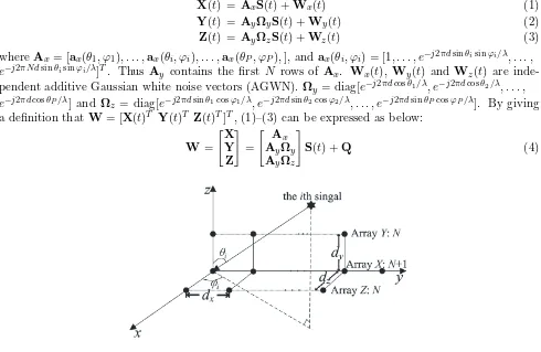
As shown in Figure 1, the array geometry is composed by a three parallel uniform linear arrays (ULAs) with the arrays named array X, array Y and array Z. ArraysY andZ are made up of N sensors, but ArrayX has one more sensor than ArrayY. We assume that the adjacent sensor distance of each array isd, which is equal to half of the wavelength of the incoming signal source, which meansd=λ/2. There are P far-field narrow-band uncorrelated source signals impinging on the array and theith source has the elevation angle θi and azimuth angleϕi. Thus, in the noisy case [5], we can obtain the output data
vector of the whole arrays at snapshottas:
X(t) = AxS(t) +Wx(t) (1) Y(t) = AyΩyS(t) +Wy(t) (2) Z(t) = AyΩzS(t) +Wz(t) (3)
whereAx= [ax(θ1, ϕ1), . . . ,ax(θi, ϕi), . . . ,ax(θP, ϕP),], and ax(θi, ϕi) = [1, . . . , e−j2πdsinθisinϕi/λ, . . . ,
e−j2πN dsinθisinϕi/λ]T. Thus A
y contains the first N rows of Ax. Wx(t), Wy(t) and Wz(t) are
inde-pendent additive Gaussian white noise vectors (AGWN). Ωy = diag[e−j2πdcosθ1/λ, e−j2πdcosθ2/λ, . . . ,
e−j2πdcosθP/λ] and Ω
z = diag[e−j2πdsinθ1cosϕ1/λ, e−j2πdsinθ2cosϕ2/λ, . . . , e−j2πdsinθPcosϕP/λ]. By giving
a definition that W= [X(t)T Y(t)T Z(t)T]T, (1)–(3) can be expressed as below:
W=
X
Y Z
=
A
x
AyΩy AyΩz
S(t) +Q (4)
Figure 1. Array model.
In short, we write Eq. (4) as W = AS +Q, where A = [ATx (AyΩy)T (AzΩz)T]T,S(t) = [S1(t), . . . ,SP(t)]T and Q= [WxT WTy WTz]T denotes the noise vector of array output.
3. MATRIX COMPLETION
which need to be recovered have low rank P obviously. Candes and Recht’s research [16] shows that the recovered data are related to the following optimization problem:
min
W W∗, subject toWij =Dij,∀(i, j) ∈Ω, (5)
where Ωis the set of indices of functional sensors, and D represents the data received from the array. The most famous algorithm to solve this problem is the singular value thresholding (SVT) method [17]. In this paper, we introduce an algorithm known as the Inexact Augmented Lagrange Multiplier (IALM) algorithm [13] to deal with it. Eq. (5) can be expressed as:
min
W W∗, subject toW+E=D, πΩ(E) = 0, (6)
whereπΩ:Rm×n→Rm×nis a projection operator which keeps the elements inΩunchanged and other elements not inΩturns into zeros. E is the error matrix. The partial augmented Lagrangian function of Eq. (6) is:
L(W,E,Y, μ) =W∗+Y,D−W−E+μ
2D−W−E
2
F. (7)
Then we can have the Inexact ALM algorithm for the MC problem by updating E under the condition thatπΩ(E) = 0 when minimizingL(W,E,Y, μ). Above all, we have Algorithm 1 as follows:
Algorithm 1 Inexact ALM algorithm for Matrix Completion Input: Dij,(i, j)∈Ω,D∈Rm×n
Output: ( ˆWk,Ek)
1: Y0 = 0;E0= 0;μ0 >0;ρ >1;k= 0. 2: whilenot converged do
3: (U,S,V) =svd(D−Ek+μ−k1Yk); 4: Wˆ k+1=USμ−1
k [S]V T;
5: Ek+1=πΩ(D−Wˆk+1+μ−k1Yk); 6: Yk+1=Yk+μk(D−Wˆ k+1−Ek+1); 7: μk+1 =ρμk;
8: k=k+ 1; 9: end while 10: return ( ˆWk,Ek).
Because of the appropriate choice ofEk,Y= 0 is always established in the iteration, and it means that the values of the unknown part retain zeros. The iteration reaches its stopping criteria as follows:
D−Wˆ k−Ek
F/DF < ε1 and dist(ϑ
Wˆ
k
∗,S)/DF < ε2, (8)
The output matrix ˆWis what we need. With the recovered matrix ˆW, we can come to the following DOA estimation part.
4. 2D-DOA
In this section, a computationally efficient azimuth and elevation angle estimation algorithm for a three-parallel uniform linear arrays [10] is applied to obtain a parameter estimation without searching computation. The algorithm, based on the propagator method (PM), can automatically pair the azimuth and elevation angles. In Section 2, we have obtained the incomplete output matrix W of the array. Then in Section 3, we get the recovered matrix ˆW which is equal to the complete output data of the array through the above procedure of matrix completion. We can partitionA firstly as follows:
whereA1 is aP×P matrix, andA2is a (3N+1−P)×P matrix. Then we can obtain aP×(3N+1−P)
propagator as:
PHA1 =A2, (10)
We introduce a matrixPe defined as Pe = [ITP P]H. In the noiseless case, PeA1 =A2. Then we
can partitionPe as:
Pe=PTx PTy PTyT, (11)
Combining Eqs. (9) and (11), we have [PT
x PTy PTy]TA1 = [ATx (AyΩy)T (AzΩz)T]T. By
introducingPx1 which has the firstN rows of Px, we can obtain:
Px1A1 = Ay (12)
PzA1 = AyΩz (13)
Then we can get P+x1Pz = A1ΩzA−11. The eigenvalues βi(i = 1,2, . . . , P) of P+x1Pz can be
obtained by doing the EVD on this equation. Ωy and Ωx can be obtained in the same way, where Ωx= diag[e−j2πdsinθ1cosϕ1/λ, e−j2πdsinθ2cosϕ2/λ, . . . , e−j2πdsinθPcosϕP/λ].
Above all, the 2D-DOA estimation algorithm is described as follows:
Algorithm 2 Modified 2D-DOA estimation algorithm for three-parallel uniform linear arrays
Input: Matrix W, and then a recoverded data ˆW is obtained by the IALM algorithm and the incomplete data W.
Output: ( ˆϕi,θˆi)
1: Compute the covariance matrix of ˆW by this formula: Rˆ
W =E[ ˆWWˆH].
2: The partition of RWˆ can be written as: RWˆ = [RWˆ1 RWˆ2], where RWˆ1 ∈ C(3N+1)×(3N+1−P).
Thus the estimation of ˆP, which is a (3N + 1−P)×P propagator matrix, can be written as: ˆ
P= (RHˆ
W1RWˆ1)− 1RH
ˆ
W1RWˆ2.
3: Then we extended propagator matrixPe= [IHP P]ˆ H.
4: Partition Pe as Pe = [PTx PTy PTz]T, where PTx ∈ C(N+1)×P,PTy ∈ CN×P,PTz ∈ CN×P. Then
importing a matrix Px1 which has the first N rows of Px, we can get a matrix Ψz by defining
Ψz =P+x1Pz. By performing EVD on Ψz, we can obtain the eigenvectors A1 and the eigenvalues
ˆ
βi ofΨz.
5: By importing a matrixPe1written asPe1 = [PTx1PTy]T, we can get a matrixBin whichB=Pe1A1.
Then we construct two new matrixes B1 and B2. B1 has the first N rows of B, and B2 has the
rest rows of B. Matrix ˆΩy is defined by ˆΩy = B+1B2. Then we can get ˆαi from the ith diagonal
element of ˆΩy.
6: Now we import a series of matrixes Px2,Py1,Py2,Pz1,Pz2, where Px2 has the lastN rows of Px;
Py1 has the firstN−1 rows ofPy;Py2 has the lastN−1 rows ofPy;Pz1 has the firstN−1 rows
ofPz; Pz2 has the last N−1 rows ofPz. Then we construct two matrixes C1 and C2 by defining
C1 = [PTx1 PTy1 PTz1]TA
1 and C2 = [PTx2 PTy2 PTz2]TA
1. ˆΩx is obtained by performing ˆΩx=C+1C2.
We can get ˆγi when we put EVD on ˆΩx.
7: We can attain the estimate of ˆϕi and ˆθi from the following equations:
ˆ
ϕi= arctan
arg(ˆγi)
arg( ˆβi)
ˆ
θi= arctan
arg( ˆβi)
arg( ˆαi) cos( ˆϕi)
5. SIMULATION RESULTS
In this section, several simulations are given to show the improvement of performance of the proposed method. We assume three uncorrelated signal sources with (ϕ1, θ1) = (20◦,10◦), (ϕ2, θ2) = (40◦,30◦)
and (ϕ3, θ3) = (60◦,50◦) impinging on the received array. Arrays Y and Z have 15 sensors, which
means that array X has 16 sensors according to the array structure. We assume that all sensors have the same probability to break down. Also we have the ability to know which sensor is broken and get their locations. After all, we take 200 snapshots for each test. By introducing a new parameter sampling rate p, which equals the percentage of working sensors in all, we can describe the damage to the array. The Mean Square Error (MSE) is defined as:
MSEθi =
E[(θi−θˆi)2]; (14)
MSEϕi = E[(ϕi−ϕˆi)2]; (15)
In the first test, we set the sampling ratepat 0.7, which means that only 70% sensor is functional in this array. And then let SNR change from 0 dB to 30 dB. Figure 2 and Figure 3 show that our proposed method has a better performance in the whole range of SNRs, and it works much better at higher SNR than that at lower SNR.
Figure 2. MSE forθ (dB). Figure 3. MSE for ϕ(dB).
In the second test, we set the SNR as 20 dB. Then let the sampling rate p change from 0.4 to 0.9. The result of DOA estimation is shown from Figure 4 and Figure 5. It is seen that this proposed method remains stable at a low sampling rate, which means that the proposed method can work well when most sensors of the array are functioned at a reasonable SNR.
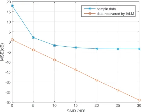
We should notice that this method also suits for other 2D-DOA methods if the shape of the array changes. In the third test, we change array into a Uniform Circular Array (UCA) and use the UCA-ESPRIT algorithm to do the DOA estimation. Then we set the sampling rate p on 0.6 and let SNR change from 0 dB to 30 dB. It is shown in Figure 6 that this proposed method can still work if the shape of array configuration is changed.
0 5 10 15 20 25 30 SNR (dB)
-30 -25 -20 -15 -10 -5 0 5 10 15 20
MSE(dB)
sample data data recovered by IALM
Figure 6. MSE for UCA array (dB).
6. CONCLUSION
In this paper, we propose a computationally efficient method for 2D-DOA estimation with a three-parallel array, which is aimed at solving the problem that when an incomplete data is received from an array, using a faster Matrix Completion method-IALM, we can get a correct 2D-DOA estimation result with the recovered data of the array. The simulation results show that the proposed algorithm has an improved performance compared to the conventional method when only a small number of sensors in the array are still working. Moreover, we can use different array configurations in practical application, and this method can still work.
Acknowledgement
This work was jointly supported by a grant from the program for New Century Excellent Talents in University under Grant NCET-13-0940, the Natural Science Foundation of Hubei Province under Grant 2014CFB791, the Research Plan Project of Hubei Provincial Department of Education under Grant T201206, and Graduate Innovative Fund of Wuhan Institute of Technology under Grant CX2015055.
REFERENCES
1. Krim, H. and M. Viberg, “Two decades of array signal processing research: The parametric approach,”IEEE Signal Processing Magazine, Vol. 13, No. 4, 67–94, 1996.
3. Wang, G., J. Xin, N. Zheng, and A. Sano, “Computationally efficient subspace-based method for two-dimensional direction estimation with L-shaped array,” IEEE Transactions on Signal Processing, Vol. 59, No. 7, 3197–3212, 2011.
4. Liang, J. and D. Liu, “Joint elevation and azimuth direction finding using L-shaped array,” IEEE Transactions on Antennas &Propagation, Vol. 58, No. 6, 2136–2141, 2010.
5. Liang, J., X. Zeng, W. Wang, and H. Chen, “L-shaped array-based elevation and azimuth direction finding in the presence of mutual coupling,”Signal Processing, Vol. 91, No. 5, 1319–1328, 2011. 6. Wu, Y., X. Pei, and H. C. So, “Utilizing principal singular vectors for 2D DOA estimation in single
snapshot case with uniform rectangular array,”International Journal of Antennas & Propagation, Vol. 2015, 1–6, 2015.
7. Wu, Y., L. Amir, J. R. Jensen, and G. Liao, “Joint pitch and DOA estimation using the ESPRIT method,”IEEE/ACM Transactions on Audio Speech&Language Processing, Vol. 23, No. 1, 32–45, 2015.
8. Reyna, A. and M. A. Panduro, “Optimization of a scannable pattern for uniform planar antenna arrays to minimize the side lobe level,”Journal of Electromagnetic Waves and Applications, Vol. 22, No. 16, 2241–2250, 2008.
9. Yuan, Q., Q. Chen, and K. Sawaya, “Accurate doa estimation using array antenna with arbitrary geometry,” IEEE Transactions on Antennas & Propagation, Vol. 53, No. 4, 1352–1357, 2005. 10. Chen, H., C. Hou, Q. Wang, L. Huang, W. Yan, and L. Pu, “Improved azimuth/elevation
angle estimation algorithm for three-parallel uniform linear arrays,” IEEE Antennas & Wireless Propagation Letters, Vol. 14, 329–332, 2015.
11. Wu, Y., G. Liao, and H. C. So, “A fast algorithm for 2-D direction-of-arrival estimation,” Signal Processing, Vol. 83, No. 8, 1827–1831, 2003.
12. Yerriswamy, T. and S. N. Jagadeesha, “Joint azimuth and elevation angle estimation using incomplete data generated by a faculty antenna array,” Signal & Image Processing, Vol. 3, No. 6, 99–114, 2012.
13. Lin, Z., M. Chen, and Y. Ma, “The augmented lagrange multiplier method for exact recovery of corrupted low-rank matrices,” Eprint Arxiv, 9, 2009.
14. Savas, B. and D. Lindgren, “Rank reduction and volume minimization approach to state-space subspace system identification,” Signal Processing, Vol. 86, No. 86, 3275–3285, 2006.
15. Iglesias, R., F. Ares, M. Fernandez-Delgado, J. Rodriguez, J. Bregains, and S. Barro, “Element failure detection in linear antenna arrays using case-based reasoning,” IEEE Antennas & Propagation Magazine, Vol. 50, No. 4, 198–204, 2008.
16. Cand`es, E. J. and B. Recht, “Exact matrix completion via convex optimization,” Foundations of Computational Mathematics, Vol. 9, No. 6, 717–772, 2008.